Understanding Python and Its Modules
Python is a versatile programming language popular for its simplicity and readability.
This section explores Python’s core programming fundamentals, its module system, and how modules are imported in Python.
Python Programming Fundamentals
Python programming is known for its straightforward syntax and dynamic typing. It handles both simple and complex tasks elegantly.
The language supports different programming paradigms, such as procedural, object-oriented, and functional programming.
Variables in Python don’t require explicit declaration; their types are inferred when a value is assigned.
Control structures like loops and conditional statements are also simple to use, making Python an excellent choice for beginners.
Python’s standard libraries and built-in functions streamline common tasks like file handling and data processing. These features make Python a powerful tool for developers across various fields.
The Module System in Python
Modules in Python are files containing Python-code that define functions, classes, and variables. They help organize code and promote reusability.
A module is created by saving Python code in a file with a .py extension.
To access a module’s content, Python programmers use the import statement. This method brings one module’s functions and classes into another, allowing seamless integration of different functionalities.
With these abilities, developers can break their code into manageable parts.
Python’s extensive support for modules enhances productivity and maintains organization during software development projects.
Core Python Modules and Import Mechanics
Python features numerous built-in modules, such as itertools, sys, and os. These modules are loaded by default and offer tools for various tasks.
To utilize a module, the import keyword is employed. For finer control, the from keyword can import specific components.
For instance, import math allows access to mathematical functions, while from math import sqrt directly imports the square root function.
Modules have their own namespace, avoiding conflicts between different functions and variables. This system is crucial for larger projects that involve various dependencies.
Setting Up the Python Environment
Setting up the Python environment efficiently is crucial for managing dependencies and project versions. This involves correctly configuring paths and deciding how to handle different Python versions.
PythonPath Configuration
The PYTHONPATH variable helps define where Python looks for modules outside its default locations. This can be crucial on systems like Windows, where file paths can vary.
The sys.path is a list that includes directories Python searches for modules. Python apps can adjust this list at runtime, but configuring PYTHONPATH beforehand ensures the environment is set up before Python starts.
Setting PYTHONPATH requires adding paths to directories containing Python modules in the environment variables. This process can be done via the command line or through system settings.
Correctly managing these paths helps avoid conflicts and ensures that scripts run smoothly by accessing the correct resources first.
Managing Python Versions
Managing Python versions is vital for maintaining compatibility across different projects.
Tools like pyenv or the built-in venv module can create isolated environments, each with its own version of Python. This is important for projects that rely on specific features or libraries.
On Windows, updating or switching between versions might require administrative privileges.
Using virtual environments not only isolates dependencies but also simplifies the process of switching projects with differing requirements.
This ensures smooth operations by preventing version mismatches.
Structured management of versions and environments allows developers to focus on development without worrying about compatibility issues.
Working with External Python Modules
Working with external Python modules allows developers to enhance their programs with additional features. By utilizing tools like pip, they can easily manage and install these modules. Understanding the structure of .py files is key to successfully integrating external code into projects.
Using pip to Install Packages
pip is Python’s package manager that simplifies the installation process of external modules. It allows users to easily add and manage different packages in their environment, making it an essential tool for anyone learning Python.
To install a package, users simply type a command such as pip install <package-name> in their terminal.
Many popular libraries are available through pip, such as NumPy for numerical computations and requests for making HTTP requests.
When installing a package, pip resolves dependencies and installs them automatically, ensuring all necessary components are available.
Using pip, developers can also update and uninstall packages, providing flexibility and control over the development environment.
Staying organized with pip is crucial, and it supports creating a requirements.txt file. This file lists all necessary packages and their versions, which can be shared across projects.
By using pip install -r requirements.txt, developers can quickly set up a consistent environment on different systems.
Understanding the .py Files
When working with external Python modules, developers often encounter .py files. These are the main files containing source code written in Python. They can include functions, classes, and other definitions that form a module or package.
These files are essential for learning how to use a module effectively. Developers can explore the code within .py files to see how specific functions are implemented and understand usage patterns.
This is especially helpful when documentation is limited or when clarifying the behavior of complex code.
Sometimes, it’s necessary to modify .py files to customize the behavior of a module. When doing so, customizing can bring specific functionality into line with project requirements. However, one must always consider compatibility issues with future updates to the module.
Understanding how .py files work and how to navigate them is crucial for successfully integrating external modules into a Python project.
Module Aliases and Namespace Management
In Python, using module aliases can simplify code by creating shortcuts for module names. It’s crucial for programmers to manage namespaces efficiently to prevent conflicts. The following subsections explore how to create aliases for modules and best practices for managing namespaces.
Creating Aliases for Modules
When working with Python modules, defining aliases can make code more readable. For instance, instead of using the full name of a module, a short alias can be used. A common example is importing the pandas library as pd.
import pandas as pd
This practice helps keep code concise, reducing clutter when repetitive module names are needed. Aliases are especially useful in large projects where module names overlap. Using a consistent alias across projects also enhances code readability.
Using standard aliases that are widely recognized minimizes confusion. For instance, np is the standard alias for numpy. Recognizable aliases improve collaboration by maintaining uniformity across different codebases.
Namespace Best Practices
Namespaces in Python act as containers for identifiers like variables and functions. Proper management prevents naming conflicts that could arise from using the same name for different objects.
When importing modules, it’s essential to manage the namespaces to avoid collisions.
By structuring and utilizing namespaces, programmers can avoid unintended interactions between different parts of a program.
For instance, using from module import function can bypass a full module name, but may lead to conflicts if two modules have functions with identical names.
Programmers should prefer importing the whole module and using an alias to access its functions or classes. This approach keeps namespaces distinct and clear, reducing potential confusion and errors.
Organizing code into packages and sub-packages with clear naming conventions also helps in managing namespaces effectively.
Data Handling with Python Modules
When handling data in Python, understanding the available data structures and analytical tools is important. Using them correctly can greatly improve the efficiency of coding tasks related to data processing. This section focuses on essential data structures and modules in Python for effective data handling and analysis.
Data Structures in Python
Python offers several data structures that allow for efficient data manipulation.
Lists are one of the most common structures, ideal for storing ordered data. They allow for easy modifications such as adding or removing elements.
Dictionaries are another powerful structure, providing a way to store data as key-value pairs. This makes data retrieval straightforward when you know the key associated with the data you need.
Sets are useful for handling unique elements and performing operations like unions and intersections efficiently.
Arrays can be managed using libraries like numpy, offering specialized features such as multidimensional arrays and high-level mathematical functions.
Each of these structures can help reduce the complexity and increase the speed of data operations in Python, making them fundamental to effective data handling.
Modules for Data Analysis
For more advanced data analysis, Python provides powerful libraries such as the pandas library.
Pandas offer data manipulation capabilities similar to a spreadsheet, allowing users to create, modify, and analyze data frames with ease.
With functionalities for handling missing data, grouping data, and computing statistics, pandas is a favorite among data analysts.
It also supports data import from various formats such as CSV, Excel, and SQL databases, making it versatile in data preparation.
In addition, tools like matplotlib and seaborn are often used alongside pandas for data visualization.
They help in creating plots and graphs, which are essential for data-driven storytelling.
By combining these tools, Python becomes a robust choice for comprehensive data analysis tasks.
Enhancing Code Maintainability and Readability
Improving the maintainability and readability of Python code involves employing effective programming paradigms and ensuring clarity in the code structure. This section explores the significance of adapting different paradigms and highlights why readable code is crucial.
Programming Paradigms and Python
Python supports multiple programming paradigms that help enhance code maintainability and readability.
Object-oriented programming (OOP) encourages code organization by using classes and objects. This leads to better reusability and simplicity, which is essential for managing larger codebases.
Functional programming, another paradigm, focuses on immutability and pure functions. As a result, the code is often more predictable and easier to test.
These practices help in reducing errors and maximizing readability.
Using paradigms like these allows developers to write cleaner code that aligns well with Python’s design philosophy.
Python’s support for various paradigms provides flexibility in choosing the best structure for the task. By using the right paradigm, developers can write more readable, maintainable, and efficient code.
The Importance of Readable Code
Readable code is vital for maintaining and scaling projects in any programming language.
Clarity in code makes it easier for other developers to understand and contribute to existing projects. It reduces the learning curve for new team members and simplifies debugging processes.
Following style guides like PEP 8 ensures consistency, helping developers focus on logic rather than syntax nuances.
Tools and best practices, like those found in resources discussing Pythonic code, offer ways to enhance code clarity.
Readable code is not just about aesthetics; it significantly affects the ease with which a codebase can be maintained and advanced.
Prioritizing readability from the start can lead to more streamlined and efficient development processes.
Scientific Computing in Python
Python is a powerful tool for scientific computing due to its extensive range of libraries. Two critical aspects are performing numerical tasks and data visualization. These topics are addressed through libraries like Numpy and Matplotlib.
Leveraging Numpy for Numerical Tasks
Numpy is essential for numerical computing in Python. It provides high-performance multidimensional arrays and tools to work with them efficiently.
Scientists use arrays to store and manipulate large datasets, which is common in scientific applications.
One key feature is broadcasting, allowing operations on arrays of different shapes without needing additional code. This helps simplify complex mathematical operations.
Numpy also offers functions for linear algebra, Fourier transforms, and random number generation.
Arrays in Numpy can be created with simple functions such as array() for lists and linspace() for generating evenly spaced numbers.
Numpy’s capabilities make it a cornerstone in scientific computing, ensuring speed and ease-of-use in data processing tasks. For those interested in diving deeper into Numpy, GeeksforGeeks covers it in greater detail.
Data Visualization Techniques
Visualizing data effectively is crucial in scientific computing. Matplotlib is a popular library providing ease in creating static, animated, and interactive plots in Python. It helps in making sense of complex data through graphical representation.
With Matplotlib, users can create line plots, scatter plots, histograms, and more. Its interface is inspired by MATLAB, making it familiar for users transitioning from those environments.
Important plot elements like labels, titles, and legends are customizable.
Example code:
import matplotlib.pyplot as plt

plt.plot([1, 2, 3, 4])
plt.ylabel('some numbers')
plt.show()
Matplotlib’s flexibility allows integration with other libraries like Pandas for data analysis. Understanding its core functions enhances anyone’s ability to present data effectively. More information about these techniques can be found at the Scientific Python Lectures site.
Integration of Python in Data Science

Python plays a crucial role in data science due to its vast ecosystem of libraries. These tools aid in data manipulation and machine learning, providing the foundation for effective data analysis and model building.
Key libraries include Pandas and Scikit-Learn, each offering unique capabilities for data scientists.
Pandas for Data Manipulation
Pandas is a powerful library for data manipulation and analysis. It provides data structures like DataFrames, which allow users to organize and explore large datasets effortlessly.
Pandas is particularly valuable for cleaning data, handling missing values, and transforming data into a more usable format.
With its intuitive syntax, it enables quick data aggregation and filtering, crucial steps for preparing data for analysis. Key features of Pandas include:
- Data Alignment: Handles missing data seamlessly.
- Grouping: Easily group and summarize data.
- Merge and Join: Combine datasets based on common fields.
By providing these functions, Pandas streamlines the data preparation process, making it easier to perform analyses needed in data science projects. Pandas is an essential tool for anyone working with data.
Machine Learning with Scikit-Learn
Scikit-Learn is a pivotal library for machine learning in Python. It is designed for a wide range of applications, from classification to regression.
Scikit-Learn provides simple tools for building predictive models, making it accessible even for beginners in data science.
It supports model selection and evaluation, allowing users to fine-tune their algorithms for improved performance. Here are key aspects of Scikit-Learn:
- Versatile Algorithms: Includes SVMs, decision trees, and more.
- Model Validation: Offers cross-validation techniques.
- Feature Selection: Helps identify the most important data attributes.
Scikit-Learn’s comprehensive suite of tools positions it as a go-to library for implementing machine learning models in Python. This makes it an integral part of data science practices.
Python for Web Development
Python is a versatile language often used in web development. It supports powerful frameworks like Flask and tools such as Beautiful Soup for web scraping.
Web Frameworks: Flask
Flask is a micro web framework written in Python. It is designed to make building web applications straightforward and quick.
Unlike bigger frameworks, Flask gives developers control over the components they want to use by keeping the core simple but allowing extensions when needed.
Flask is based on the WSGI toolkit and Jinja2 template engine. It is lightweight, making it easy to learn and ideal for small to medium-sized projects.
Flask does not enforce a specific project layout or dependencies, offering flexibility.
Developers often choose Flask when they desire to have a modular design for their web application. It allows them to organize their code in a way that makes sense for their specific needs.
Web Scraping with Beautiful Soup
Beautiful Soup is a library that makes it easy to scrape web pages. It can parse HTML and XML documents, creating a parse tree for web scraping tasks like extraction and navigation of data.
Beautiful Soup provides Pythonic idioms for iterating, searching, and modifying the parse tree.
For web developers, Beautiful Soup is useful when they need to retrieve data from web pages quickly and efficiently.
It can turn even the most tangled HTML into a manageable parse tree. It supports many parsers, but working with Python’s built-in HTML parser makes this tool very straightforward.
This library is widely used for tasks like data mining and creating automated data collection tools.
Advanced Python Modules for Machine Learning
Python offers strong modules like TensorFlow and Keras that are essential for deep learning. They enable the construction and training of neural networks, providing tools needed to develop sophisticated machine learning applications.
TensorFlow and Keras for Deep Learning
TensorFlow is a robust open-source framework ideal for tasks involving neural networks. It supports computations on both CPUs and GPUs, making it highly versatile for various environments.
Its core strengths include flexibility and scalability, catering to both research and production needs.
TensorFlow facilitates intricate model building with its vast collection of tools and libraries.
Keras, often used alongside TensorFlow, offers a simpler API for building and training deep learning models. It is particularly popular because it allows users to prototype quickly without deep diving into the complicated details of backend computations.
Keras supports layers and models and is efficient for trying out new models rapidly.
Constructing Neural Networks
Developing neural networks with these tools involves several steps like defining layers, compiling models, and specifying optimization strategies.
TensorFlow provides robust support for customizing neural networks, making it easier to tailor models to specific needs by adjusting layers, activations, and connections.
Keras simplifies the network construction process with its user-friendly interface. It allows for quick adjustments to various elements such as input shapes and layer types.
Users can effortlessly stack layers to create complex architectures or modify settings to enhance performance.
Interacting with the Python Package Index
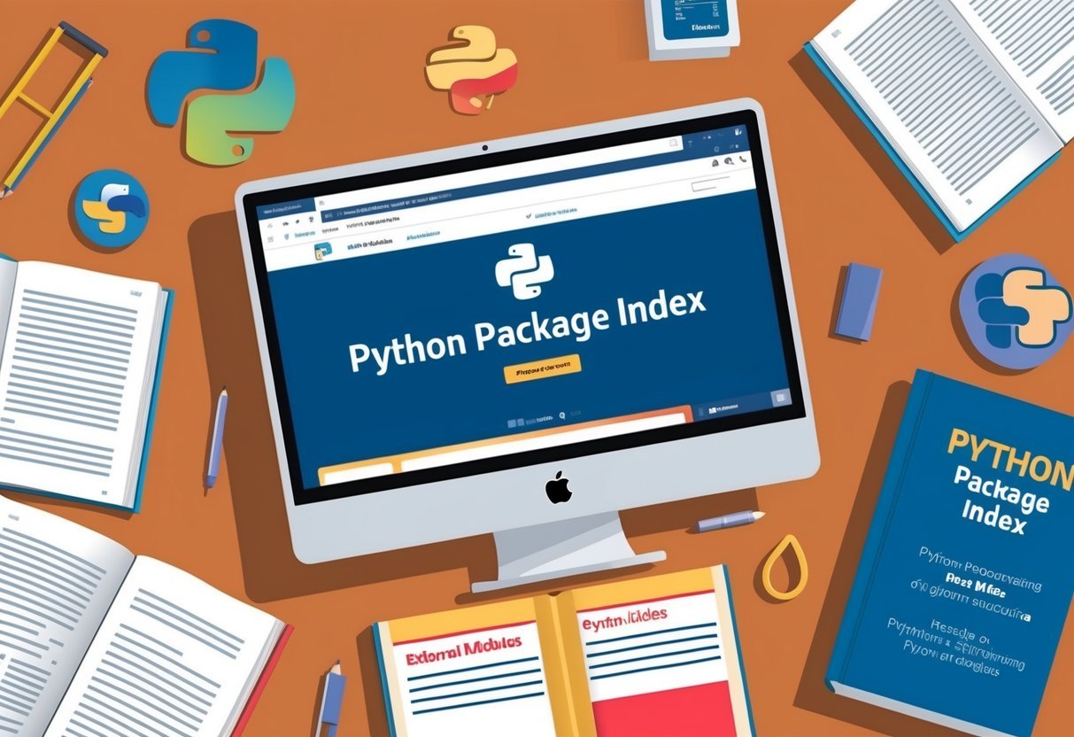
The Python Package Index (PyPI) is a hub where users can discover a wide range of packages to enhance their projects. It also offers an opportunity for developers to share their work by contributing packages to the community.
Finding Python Packages
PyPI serves as a repository where users can find and install packages made by the Python community. Tools like pip help in fetching these packages directly from PyPI.
Users can browse and explore packages on the PyPI website, which provides details about each package, including its dependencies and usage. Many packages also host their source code on GitHub, allowing users to review code and participate in development.
Contributing to Python Packages
Developers looking to contribute to PyPI can package their code and submit it to the index for community use.
Creating a package involves preparing code and documentation, and using tools like setuptools to handle packaging requirements. Detailed instructions for uploading packages help guide developers through sharing their projects on PyPI.
Often, developers collaborate using platforms like GitHub to maintain and discuss improvements to their projects, fostering a collaborative environment.
Computer Vision and Image Processing with Python
Python, with its simplicity and power, offers robust tools for computer vision and image processing. At the forefront of these is OpenCV, a comprehensive library that enables the manipulation and understanding of visual data. This provides both beginners and experts with a suite of tools to create complex applications.
Understanding OpenCV
OpenCV is a powerful, open-source library designed for computer vision and image processing tasks. It supports Python, making it accessible to a wide range of users.
The library can handle various functions such as image recognition, object detection, and video analysis.
One of OpenCV’s strengths is its ability to convert images and videos into a format that can be easily processed. For example, it can convert colored videos to gray-scale efficiently, a common step in many image processing tasks.
The handy APIs in OpenCV allow developers to write efficient code for real-time applications, leveraging multicore processors effectively.
For those new to this field, OpenCV provides a strong foundation for learning and experimentation. It integrates well with libraries such as NumPy, allowing for powerful mathematical operations on image data.
OpenCV also supports machine learning tasks, forming a bridge between computer vision and AI.
Advanced users can take advantage of OpenCV’s GPU acceleration features, which enhance performance for resource-intensive tasks. This is crucial for projects requiring high efficiency and speed.
Overall, OpenCV remains a versatile and essential library for those venturing into computer vision with Python. For additional tutorials and resources on OpenCV, developers can explore GeeksforGeeks or the OpenCV University.
Frequently Asked Questions

Learning about Python external modules can greatly enhance programming projects. Understanding how to find, install, and manage these modules is important for both beginner and advanced developers.
How can I find and install external modules in Python?
External modules in Python can be found on the Python Package Index (PyPI). To install them, one can use the pip command in a terminal or command prompt.
For example, to install a module like NumPy, the user can execute pip install numpy.
Which external modules are essential for beginners in Python development?
Beginners might start with modules that simplify common tasks. Popular choices include NumPy for numerical computations and matplotlib for creating visualizations.
These modules are user-friendly and have rich documentation, making them great choices for newcomers.
What are the differences between built-in and external Python modules?
Built-in modules are part of the Python standard library and do not require installation. External modules, on the other hand, are developed by third parties and need to be downloaded and installed separately using tools like pip.
What are some examples of popular external modules used in Python projects?
Some widely used external modules in Python projects include requests for handling HTTP requests, Pandas for data manipulation, and Flask for web development.
These modules offer specialized functionality that can significantly boost development efficiency.
Where can beginners find resources or tutorials for learning about external Python modules?
Beginners can explore platforms like GeeksforGeeks for articles and guides. Additionally, sites like Stack Overflow provide answers to specific questions, and the official Python documentation offers comprehensive information about module usage.
How do you manage and update external Python modules in a project?
To manage and update external modules, tools like pip are essential.
Users can check for outdated packages with pip list --outdated and then update them using pip install --upgrade package-name.
Version control systems also help maintain module consistency in project environments.