Weekend Bootcamps

Understanding Ridge Regression

Ridge regression is a powerful technique used in statistics and machine learning. It is particularly useful for dealing with multicollinearity, where predictor variables are highly correlated with each other.

This model modifies the linear regression by adding a penalty to the size of the coefficients.

The main idea is to limit the size of the coefficients using regularization. Ridge regression applies an L2 regularization penalty. This means it adds a term to the loss function, which is the square of the magnitude of coefficients.

This penalty term is called the ridge regression penalty.

This penalty causes shrinkage, or the reduction of the magnitude of coefficients. By doing so, it prevents overfitting, making the model more robust when making predictions.

Large coefficients are scaled down, which helps when the model needs to generalize from the given data.

A key advantage of ridge regression is its ability to handle numerous predictor variables and make models less sensitive to noise. In addition, all predictors remain in the model, avoiding complete exclusion unlike other methods such as Lasso regression.

Regularization involves tuning a hyperparameter, usually denoted as alpha (α). This parameter controls the strength of the penalty.

A higher alpha increases the penalty, further shrinking the coefficients. Adjusting alpha carefully can significantly impact model performance.

In applications, ridge regression is widely used in various fields, including finance, biology, and social sciences, where it helps to improve model stability and interpretability when faced with complex data structures.

Fundamentals of Linear Regression

Linear regression is a key technique in statistics for modeling the relationship between a dependent variable and one or more independent variables. It predicts numerical outcomes, serving as a foundational tool in regression analysis.

Exploring Ordinary Least Squares (OLS)

Ordinary Least Squares (OLS) is the most common method for estimating the parameters in a linear regression model. It works by minimizing the sum of the squared differences between the observed values and the values predicted by the model.

In simple linear regression, there is one dependent variable and one independent variable. The relationship is expressed using a linear equation.

OLS estimates help in determining the line of best fit for the data, offering insights into the dependence between variables.

Regularization in Regression Models

Regularization is a technique in regression models that helps prevent overfitting by adding a penalty term to the loss function. This helps in producing models that generalize better on unseen data.

The two primary types of regularization are L1 and L2, which add different penalties to the model parameters.

L1 vs. L2 Regularization

L1 Regularization, also known as Lasso, adds an absolute value penalty to the loss function. This results in some coefficients being reduced to zero, effectively performing feature selection.

Lasso is useful when the dataset has many features, and it aims to find the most impactful ones. Its primary advantage is that it creates sparse models that are easier to interpret.

L2 Regularization, known as Ridge, adds a squared magnitude penalty to the loss function. Unlike L1, Ridge does not lead to zero coefficients, but rather shrinks them proportionally.

This is beneficial when dealing with multicollinearity, where features are highly correlated. Ridge is favored for scenarios where all features contribute to the prediction, albeit possibly weakly.

For situations where neither Lasso nor Ridge alone is suitable, Elastic Net combines both L1 and L2 penalties.

It provides the benefits of both regularization methods. Elastic Net is particularly effective when there are many correlated predictors, balancing between feature selection and coefficient shrinkage. This results in a more flexible model suitable for a wider range of data scenarios.

Elastic Net Regression Explained

Elastic Net regression combines the strengths of Ridge and Lasso regression to improve model performance. It is particularly useful in datasets with highly correlated features or when the number of predictors exceeds observations.

Combining Strengths of Ridge and Lasso

Elastic Net uses a mixing parameter to balance the strengths of Ridge and Lasso regression. Ridge regression minimizes the sum of squared coefficients, effectively managing multicollinearity and stabilizing models.

On the other hand, Lasso regression can lead to sparse solutions by reducing some coefficients to zero, helping with feature selection.

The mixing parameter, often denoted as alpha (α), controls the contribution of each method.

When the parameter is set to zero, the model acts as Ridge regression, while a value of one turns it into Lasso. Varying alpha between these extremes allows Elastic Net regression to handle situations where neither Ridge nor Lasso alone would suffice.

This flexibility makes Elastic Net effective in situations with numerous features and complex relationships. The combination of L1 (Lasso) and L2 (Ridge) penalties enhances predictive performance and model interpretability by selecting relevant features and reducing overfitting.

This regularization technique is widely used in fields like bioinformatics, finance, and any area dealing with complex datasets.

Analyzing Bias-Variance Tradeoff

The bias-variance tradeoff is a crucial concept in machine learning and statistics. It balances two types of errors in model prediction—bias and variance. Bias refers to the error introduced when a model makes assumptions about the data, potentially leading to underfitting.

Variance captures how much the model’s predictions change with different training data. High variance can cause the model to become overly complex, known as overfitting. This occurs when the model fits the training data too closely, capturing noise rather than the intended outputs.

Improving model interpretability requires finding the right balance. High bias often means missed patterns while high variance leads to sensitivity to noise.

The goal of this tradeoff is to achieve a model that can generalize well to new data.

Generalization is the model’s ability to perform accurately on unseen data, indicating effective learning. Regularization methods like ridge and Lasso help manage this tradeoff by adding penalty terms to the cost function, keeping coefficients small.

These methods adjust the parameter size to keep bias and variance in check, improving the model’s performance.

For further reading, L2 regularization used in ridge regression is detailed here. This highlights the role of regularization in addressing model issues related to the bias-variance tradeoff.

Dealing with Collinearity in Data

When analyzing data, dealing with multicollinearity is crucial. Multicollinearity occurs when variables are highly correlated, making it difficult to identify the individual effect of each variable.

This can lead to unstable estimates in regression models.

A common strategy to handle multicollinearity is using Ridge Regression. Ridge Regression introduces a penalty to the model’s coefficients, controlling the impact of correlated variables by shrinking their values. This helps in stabilizing the estimates and improving predictions.

Lasso Regression is another technique that helps in selecting relevant features. By applying a penalty, Lasso can reduce less important coefficients to zero, effectively removing them from the model.

This aids in simplifying the model by excluding irrelevant features and focusing on those that matter most.

The Elastic Net method combines features of both Ridge and Lasso Regression, providing a balanced approach. It uses penalties to manage both correlated variables and irrelevant features.

Elastic Net is particularly useful when dealing with a large number of predictors, some of which could be correlated or not significant.

In practice, it’s essential to detect multicollinearity before applying these techniques.

Checking the correlation matrix or using Variance Inflation Factor (VIF) can help identify pairs or groups of variables that are highly correlated.

Once detected, these methods can be applied to improve the reliability and performance of regression models.

Feature Selection and Importance

Feature selection is crucial in regression analysis. It helps create models that are easy to interpret and predict accurately by keeping only the most important features.

When datasets have many variables, it’s essential to identify which ones have the most impact on the target variable.

Ridge Regression is a technique used to shrink coefficients and reduce model complexity. It helps in minimizing the influence of irrelevant features but does not perform feature selection inherently.

Instead, it keeps all variables but reduces their impact, which prevents overfitting.

Lasso Regression, on the other hand, can shrink some coefficients to zero. This means it can effectively select a subset of features by removing irrelevant features, making models more interpretable.

The ability to eliminate variables makes lasso effective when there are many predictors.

Elastic Net combines the strengths of ridge and lasso. It uses both L1 and L2 penalties to handle highly correlated features and selects variables.

This makes it suitable for datasets where feature selection is important, and multicollinearity is present. More information on Elastic Net can be found at Elastic Net Regression.

Incorporating these methods in regression allows for more accurate predictions while maintaining simplicity. Each method has its role depending on the dataset and the problem at hand. By understanding how each approach manages feature importance, better models can be developed.

Assessing Model Performance

Evaluating the effectiveness of Ridge Regression involves understanding how well the model predicts new data. Metrics like mean squared error (MSE) and R², along with techniques like cross-validation, provide insight into the model’s predictive power.

Cross-Validation Techniques

Cross-validation is a critical method for assessing model performance in machine learning algorithms. It involves splitting the dataset into several parts or “folds.” Each fold serves as both a training and testing set at different times, which helps validate the model’s performance.

A common approach is k-fold cross-validation, where the dataset is divided into k subsets. The model trains on k-1 subsets and tests on the remaining one, cycling through all folds.

This technique provides a more accurate estimate of performance metrics, such as mean squared error (MSE) and R², by ensuring that each data point is used for both training and testing.

Cross-validation helps in handling variance and bias, leading to a better assessment of the model’s true predictive power.

Optimization of Hyperparameters

Optimizing hyperparameters is crucial in improving model accuracy. It involves finding the best settings, like the alpha parameter, that can significantly enhance the performance of ridge and lasso regression models.

Choosing the Right Alpha Parameter

The alpha parameter is an essential element in Elastic Net and tuning it properly can make a big difference.

In this context, alpha controls the balance between ridge (L2) and lasso (L1) penalties, impacting model regularization.

To find the best alpha, cross-validation is a reliable method.

By testing different alpha values on subsets of data, it determines which configuration results in the lowest prediction error.

Generally, starting with a wide range and narrowing down based on performance is effective.

Many experts recommend using automated tools like GridSearchCV in Python’s scikit-learn library to streamline this process.

These tools facilitate evaluating multiple values systematically, aiding in the selection of optimal hyperparameters for improved model performance.

Machine Learning Tools for Ridge and Elastic Net

Understanding the tools for implementing ridge and elastic net regression is crucial in machine learning and data science.

Using libraries like scikit-learn in Python, users can efficiently apply these techniques to enhance their models.

Working with Scikit-Learn

Scikit-learn is a powerful library in Python that is widely used in machine learning.

It provides tools for implementing both ridge and elastic net regression. These regression techniques help in handling multicollinearity and improving prediction accuracy by regularizing the model.

In scikit-learn, the Ridge and ElasticNet classes are used to implement these models.

Users can easily specify parameters like the regularization strength for ridge regression or mix ratio for elastic net regression.

The library also offers functions like GridSearchCV for tuning model parameters, which is essential for optimizing model performance.

By taking advantage of these features, users can build robust predictive models efficiently.

Applications of Ridge Regression and Elastic Net

Ridge regression and elastic net regression are valuable in various industries. They are particularly useful in bioinformatics, finance, and marketing for addressing specific data challenges and improving model performance.

Case Studies in Various Industries

Bioinformatics
In bioinformatics, ridge regression is used for gene selection.

Identifying relevant genes linked to diseases is crucial, and ridge regression helps in managing the complexity of high-dimensional genetic data.

Elastic net regression combines penalties from both ridge and lasso methods, enhancing its ability to handle correlated variables effectively.

Finance
In finance, these regression techniques help in predicting stock prices and managing risks.

Ridge regression deals with multicollinearity, ensuring more accurate financial models.

Elastic net provides a balanced approach by controlling variances and sparse solutions, which is valuable in financial decision-making.

Marketing
In marketing, customer segmentation and sales forecasting benefit from elastic net regression.

It manages datasets with numerous predictors, enhancing prediction accuracy.

The combined regularization helps in selecting the most influential marketing variables, leading to strategic decision-making in campaigns.

Handling High-Dimensional Data

High-dimensional data can pose significant challenges during analysis because it often leads to high variance in model predictions.

Traditional methods might struggle with such complexity, resulting in models that are less reliable.

Ridge Regression is a robust method to address some of these issues.

By adding an L2 penalty, it helps in producing a simpler model that reduces high variance, but it might still struggle with bias.

Elastic Net Regression is particularly useful for handling high-dimensional datasets.

It combines the strengths of both ridge regression and Lasso, offering a balanced approach. This makes it effective when dealing with correlated predictors and feature selection.

Here’s a brief comparison of methods:

Method	Benefits	Challenges
Ridge Regression	Reduces variance	May increase bias
Elastic Net	Handles correlations	Can be complex

In scenarios where data has many features, these techniques ensure that the models remain robust and predictive. This balance is critical in models involving many variables, ensuring predictions remain accurate and useful.

High-dimensional data needs methods that maintain efficiency and reliability. Ridge regression and elastic net regression cater to these requirements, providing tools for those working with complex datasets.

Frequently Asked Questions

Ridge and elastic net regression are important techniques in statistics and machine learning. They help improve model performance and interpretation. Understanding how to implement these methods and their strengths for certain datasets provides valuable insights for practical applications.

What distinguishes ridge regression from elastic net regression?

Ridge regression uses an L2 regularization term, which shrinks coefficients towards zero but never makes them zero. Elastic net regression combines both L1 and L2 regularization, offering a penalty system that can shrink some coefficients to zero and, thus, select variables more effectively, especially with correlated features.

How is the elastic net regression model implemented in Python?

In Python, elastic net regression can be implemented using libraries like scikit-learn.

The ElasticNet class allows setting parameters such as alpha and l1_ratio to control the mix of L1 and L2 regularization.

This flexible approach makes it easier to fine-tune models for specific datasets.

What are the typical use cases for elastic net regression?

Elastic net regression is well-suited for datasets with many features, especially when they are highly correlated.

For instance, in genetics, where multiple predictors might be related, elastic net helps select relevant ones.

It’s also useful when the number of predictors exceeds observations, as it handles overfitting effectively.

How do you interpret the coefficients of an elastic net regression model?

The coefficients in an elastic net model indicate the strength and direction of the relationship between predictor variables and the target variable.

A zero coefficient means the feature is not used in the prediction. Non-zero coefficients provide information on the importance and effect size of variables.

What are the limitations of elastic net regression compared to other linear models?

Elastic net regression may require careful tuning of hyperparameters, such as alpha and l1_ratio.

This process can be computationally intensive.

It’s also sensitive to the choice of these parameters, impacting model performance.

Compared to simpler models, it might not be ideal for datasets with limited features.

How does one select the tuning parameters for an elastic net regression?

Tuning parameters for elastic net involves finding the optimal values of alpha and l1_ratio.

Techniques like cross-validation are commonly used to test different values.

Using the cross-validation results helps determine the best parameters that minimize prediction errors, improving the model’s accuracy and generalization.

Understanding CTEs in T-SQL

Common Table Expressions (CTEs) in T-SQL help simplify complex queries and enhance code readability. They allow developers to define temporary result sets within queries. This makes it easier to work with intricate data operations.

Definition and Advantages of Common Table Expressions

Common Table Expressions, or CTEs, are temporary result sets defined in SQL Server using the WITH clause. They are used to simplify and organize complex queries. Unlike derived tables, CTEs can be referenced multiple times within the same query. This makes code easier to understand and maintain.

One important advantage of CTEs is their ability to improve code readability. They allow for the breakdown of complex queries into more manageable parts. This feature is particularly useful when dealing with subqueries or recursive operations. CTEs also enhance performance by reducing repetition in SQL code.

CTE Syntax Overview

The syntax of a CTE involves using the WITH clause followed by the CTE name and the query that defines it. A simple example might look like this:

WITH EmployeeCTE AS (
    SELECT EmployeeID, FirstName, LastName
    FROM Employees
)
SELECT * FROM EmployeeCTE;

Here, EmployeeCTE acts as a temporary view in the SQL query. It starts with the keyword WITH, followed by the CTE name, and the query enclosed in parentheses. This structure makes the CTE accessible in subsequent queries, promoting cleaner and more organized SQL statements.

Anatomy of a Simple CTE

A simple CTE breaks down a query into logical steps. Consider this basic structure:

WITH SalesCTE AS (
    SELECT ProductID, SUM(Quantity) AS TotalQuantity
    FROM Sales
    GROUP BY ProductID
)
SELECT * FROM SalesCTE WHERE TotalQuantity > 100;

In this scenario, SalesCTE is defined to summarize sales data. It calculates the total quantity sold for each product. Once established, the CTE is queried again to filter results. This step-by-step approach makes the logic transparent and the SQL code more readable and modular.

Basic CTE Queries

Common Table Expressions (CTEs) are useful tools in T-SQL for simplifying complex queries. They help organize code and improve readability. A CTE can be used with SELECT, INSERT, UPDATE, and DELETE statements to manage data efficiently. Here’s how each works within CTEs.

Crafting a Select Statement within CTEs

A SELECT statement within a CTE allows for temporary result sets that are easy to reference. To create one, use the WITH keyword followed by the CTE name and the SELECT query:

WITH EmployeeData AS (
    SELECT EmployeeID, FirstName, LastName
    FROM Employees
)
SELECT * FROM EmployeeData;

This example defines EmployeeData, which can be queried as a table. CTEs improve readability and make code cleaner, especially when dealing with complex joins or aggregations.

Using CTEs with Insert Statements

INSERT statements add new records. CTEs can prepare the dataset for insertion into a target table. For instance:

WITH NewData AS (
    SELECT 'John', 'Doe', 'john.doe@example.com'
)
INSERT INTO Employees (FirstName, LastName, Email)
SELECT * FROM NewData;

This takes the specified data and inserts it into the Employees table. The CTE allows the source data to be easily modified or expanded without changing the main insert logic.

Updating Data with CTEs

CTEs are helpful in organizing complex UPDATE operations. They provide a clearer structure when the updated data depends on results from a select query:

WITH UpdatedSalaries AS (
    SELECT EmployeeID, Salary * 1.10 AS NewSalary
    FROM Employees
    WHERE Department = 'Sales'
)
UPDATE Employees
SET Salary = NewSalary
FROM UpdatedSalaries
WHERE Employees.EmployeeID = UpdatedSalaries.EmployeeID;

Here, the CTE calculates updated salaries for a particular department. This simplifies the update process and makes the code more maintainable.

Deleting Records Using CTEs

For DELETE operations, CTEs can define the subset of data to be removed. This makes it easy to specify only the needed criteria:

WITH OldRecords AS (
    SELECT EmployeeID
    FROM Employees
    WHERE HireDate < '2010-01-01'
)
DELETE FROM Employees
WHERE EmployeeID IN (SELECT EmployeeID FROM OldRecords);

This example removes employees hired before 2010. The CTE targets specific records efficiently, and the logic is easy to follow, reducing the chance of errors.

Implementing Joins in CTEs

Implementing joins within Common Table Expressions (CTEs) helps in organizing complex SQL queries. This section explores how inner and outer joins work within CTEs, providing a clearer path to refined data retrieval.

Inner Joins and CTEs

When using inner joins with CTEs, the goal is to combine rows from multiple tables based on a related column. This is useful for filtering data to return only matching records from each table.

Consider a scenario where a CTE is used to extract a specific subset of data. Inside this CTE, an inner join can link tables like employees and departments, ensuring only employees in active departments are selected.

The syntax within a CTE starts with the WITH keyword, followed by the CTE name and a query block. Inside this block, an inner join is used within the SELECT statement to relate tables:

WITH EmployeeData AS (
    SELECT e.Name, e.DepartmentID, d.DepartmentName
    FROM Employees e
    INNER JOIN Departments d ON e.DepartmentID = d.ID
)

Here, the INNER JOIN ensures that only rows with matching DepartmentID in both tables are included.

Outer Joins within CTE Structure

Outer joins in a CTE structure allow retrieval of all rows from the primary table and matched rows from the secondary table. This setup is beneficial when needing to display unmatched data alongside matched results.

For instance, if a task is to find all departments and list employees belonging to each—while also showing departments without employees—an outer join can be used. This involves a LEFT JOIN within the CTE:

WITH DeptWithEmployees AS (
    SELECT d.DepartmentName, e.Name
    FROM Departments d
    LEFT JOIN Employees e ON d.ID = e.DepartmentID
)

The LEFT JOIN retrieves all department names and includes employee data where available. Unmatched departments are still displayed with NULL for employee names, ensuring complete department visibility.

Complex CTE Queries

Complex CTE queries involve advanced techniques that enhance SQL efficiency and readability. They allow for the creation of sophisticated queries using multiple CTEs, combining CTEs with unions, and embedding subqueries.

Managing Multiple CTEs in a Single Query

When working with multiple CTEs, organizing them properly is crucial. SQL allows defining several CTEs within a single query, each separated by a comma. This method enables the SQL engine to process complex logic step by step.

For instance, a developer can create one CTE for filtering data and another for aggregating results. Managing multiple CTEs in a query helps break down complicated logic into more digestible parts and improve clarity.

Leveraging Union and Union All with CTEs

Incorporating UNION and UNION ALL with CTEs can be particularly useful for combining results from multiple queries. The UNION operator merges results but removes duplicates, while UNION ALL includes all entries, duplicates intact.

Using these operators with CTEs allows for seamless integration of diverse datasets. Developers can quickly perform comprehensive data analyses by combining tables or data sets, which would otherwise require separate queries or complex joins.

Applying Subqueries in CTEs

Subqueries within CTEs add a layer of flexibility and power to SQL queries. A subquery permits additional data processing and can be a foundation for a CTE.

For example, you might use a subquery within a CTE to identify records that meet specific conditions. By doing so, the outer query can focus on further details, improving both performance and clarity. When CTEs involve subqueries, it is important to ensure they are optimized to prevent performance lags.

Recursive CTEs Explained

Recursive Common Table Expressions (CTEs) are powerful tools in T-SQL for handling complex queries involving hierarchies and repeated processes. Understanding how to write them effectively can help avoid common pitfalls like infinite loops.

Basics of Recursive CTEs

A Recursive CTE is a query that references itself. It consists of two parts: an anchor member and a recursive member.

The anchor member initializes the CTE, and the recursive member repeatedly executes, each time referencing results from the previous iteration.

Anchor Member

This part sets the starting point. For example, it begins with a base record.

Recursive Member

It uses recursion to pull in rows relative to the data retrieved by the anchor member.

When the recursive query runs, it continues processing until no more data is left to evaluate. This makes it ideal for queries where you need to connect related rows.

Building Hierarchies with Recursive Queries

Recursive CTEs are well-suited for hierarchical structures, like organizational charts or folder trees. They efficiently traverse a hierarchical relationship and organize records in a clearly defined order.

To build such structures, define a parent-child relationship within the data.

The CTE starts with a root node (row), then iteratively accesses child nodes. This method is extremely useful in databases where relationships can be defined by IDs.

When executing, the CTE retrieves a row, retrieves its children, and continues doing so until no children remain. This layered approach allows for easy visualization of parent-child relationships.

Preventing Infinite Loops in Recursion

Infinite loops can be a risk. They occur when a recursive CTE continually refers to itself without terminating. To prevent this, two main strategies are employed.

MAXRECURSION

Use the MAXRECURSION option to limit the number of recursive calls. For example, setting OPTION(MAXRECURSION 100) will stop recursion at 100 levels, preventing infinite loops.

Stop Conditions

Implement checks within the CTE to stop recursion naturally.

By using conditions to exclude rows that should not continue, it limits how far recursion extends.

These strategies ensure that queries execute efficiently without entering endless cycles, protecting both data and system resources.

Advanced CTE Applications

Advanced Common Table Expressions (CTEs) can transform how data is processed and analyzed in SQL Server. They offer efficient solutions for dynamic reporting, pivoting data, and removing duplicate information. This guide explores these applications to enhance data management strategies.

CTEs for Pivoting Data in SQL Server

Pivoting data is a method used to transform rows into columns, simplifying data analysis. In SQL Server, CTEs can streamline this process.

By defining a CTE, users pre-select the necessary data before applying the PIVOT function. This pre-selection reduces complexity in the final query, making it more readable and efficient.

Pivoting helps in scenarios where data needs restructuring to create reports or feed into applications.

Using CTEs before the pivot operation can significantly improve performance, especially with large datasets, by organizing data logically beforehand. This approach is suitable for scenarios where data is stored in time-series formats and must be presented in a different layout.

Using CTEs for Dynamic Reporting

Dynamic reporting requires adaptable queries to respond to changing user inputs or datasets.

CTEs in SQL Server are ideal for this. They can simplify complex queries and improve readability.

For dynamic reporting, a CTE can break down a large query into manageable parts, making adjustments easier.

They can also be used to prepare data sets by filtering or aggregating data before the main query.

This organization leads to faster query execution and more responsive reports.

Furthermore, when handling multiple datasets, CTEs provide a consistent structure, ensuring that reports remain accurate and relevant.

Data Deduplication Techniques with CTEs

Data deduplication is essential to maintain the integrity and quality of databases.

With CTEs, deduplication becomes straightforward by temporarily organizing duplicated data for later removal.

By using a CTE, users can first define criteria for duplicate detection, such as identical records in primary key fields or other identifiers.

After identifying duplicates, it’s easy to apply filters or delete statements to clean the data.

This method helps maintain clean datasets without resorting to complex procedures.

Additionally, when combined with SQL Server’s ROW_NUMBER() function, CTEs can effectively rank duplicates, allowing precise control over which records to keep.

This technique not only optimizes storage but also ensures that data remains consistent and reliable.

Performance Considerations for CTEs

Performance in SQL queries is crucial when working with large datasets.

Evaluating the differences between common table expressions (CTEs) and temporary tables helps enhance efficiency.

Exploring how to optimize CTE queries can significantly boost overall execution speed and resource management.

Comparing CTE Performance with Temporary Tables

CTEs and temporary tables both serve the purpose of organizing data. A key difference lies in their scope and lifetime.

CTEs are embedded in a SQL statement and exist only for the duration of that statement. They offer a tidy structure, which makes them readable and easy to manage.

This makes CTEs ideal for complex queries involving joins and recursive operations.

Temporary tables, in contrast, are more versatile and can be reused multiple times within a session or script. This reusability could potentially lead to better performance in iterative operations where the same data set is repeatedly accessed.

However, temporary tables may require careful management of SQL resources to avoid any potential system overhead.

Deciding between CTEs and temporary tables depends largely on the use case, query complexity, and performance needs.

Optimization Strategies for CTE Queries

Optimizing CTEs involves several strategies.

An important method is minimizing the data scope by selecting only the necessary columns and rows. This reduces memory usage and speeds up query execution.

Indexes can help improve performance, even though they’re not directly applied to CTEs. Applying indexes on the tables within the CTE can enhance the query performance significantly by reducing execution time.

Another strategy is evaluating execution plans frequently. By analyzing these plans, developers can identify bottlenecks and optimize query logic to improve performance.

Adjusting query writing approaches and testing different logic structures can lead to more efficient CTE performance.

Integrating CTEs with SQL Data Manipulation

Integrating Common Table Expressions (CTEs) with SQL data manipulation provides flexibility and efficiency.

By using CTEs in SQL, complex queries become more manageable. This integration is especially useful when combining CTEs with aggregate functions or merge statements.

CTEs with Aggregate Functions

CTEs simplify working with aggregate functions by providing a way to structure complex queries.

With CTEs, temporary result sets can be created, allowing data to be grouped and summarized before final query processing.

This step-by-step approach helps in calculating sums, averages, and other aggregate values with clarity.

For instance, using a CTE to first select a subset of data, such as sales data for a specific period, makes it easier to apply aggregate functions, like SUM() or AVG(). This method improves readability and maintenance of SQL code.

Moreover, CTEs enhance performance by allowing SQL Server to optimize execution plans. Because the CTE provides a clear structure, the server can handle queries more efficiently.

This is particularly beneficial when dealing with large datasets, as it reduces complexity and improves execution time.

Merge Statements and CTEs

Merge statements in SQL are used to perform inserts, updates, or deletes in a single statement based on data comparison.

When combined with CTEs, this process becomes even more effective.

A CTE can be used to select and prepare the data needed for these operations, making the merge logic cleaner and more understandable.

For example, using a CTE to identify records to be updated or inserted helps streamline the merge process. This approach organizes the data flow and ensures that each step is clear, reducing the likelihood of errors.

The integration of CTEs also helps in managing conditional logic within the merge statement. By using CTEs, different scenarios can be handled efficiently, leading to robust and flexible SQL code.

This makes maintaining and updating the database simpler and less error-prone.

Enhancing SQL Views with CTEs

Common Table Expressions (CTEs) are useful tools in SQL for enhancing efficiency and readability when creating complex queries. They enable developers to build more dynamic and understandable views.

Creating Views Using CTEs

Creating views in SQL using CTEs allows for cleaner and easier-to-maintain code.

A CTE defines a temporary result set that a SELECT statement can reference. When a view is created with a CTE, the CTE’s ability to break down complex queries into simpler parts makes updates and debugging more straightforward.

Consider a CTE named SalesByRegion that aggregates sales data by region. By using CREATE VIEW, this CTE can be repeatedly referenced without the need to write the complex logic each time.

WITH SalesByRegion AS (
    SELECT Region, SUM(Sales) AS TotalSales
    FROM SalesData
    GROUP BY Region
)
CREATE VIEW RegionalSales AS
SELECT * FROM SalesByRegion;

This approach separates the logic for calculating sales from other operations, enhancing clarity and reducing errors.

Nested CTEs in Views

Nested CTEs increase flexibility in SQL views. They allow one CTE to reference another, building layered queries that are still easy to follow.

This can be especially helpful in scenarios where multiple preprocessing steps are needed.

Suppose a query requires calculating both sales by region and average sales per product. Using nested CTEs, each step can be processed separately and combined seamlessly:

WITH SalesByRegion AS (
    SELECT Region, SUM(Sales) AS TotalSales
    FROM SalesData
    GROUP BY Region
), AverageSales AS (
    SELECT ProductID, AVG(Sales) AS AvgSales
    FROM SalesData
    GROUP BY ProductID
)
CREATE VIEW DetailedSales AS
SELECT sr.Region, sr.TotalSales, a.AvgSales
FROM SalesByRegion sr
JOIN AverageSales a ON sr.Region = a.ProductID;

The readability of layered CTEs makes SQL management tasks less error-prone, as each section of the query is focused on a single task.

By utilizing nested CTEs, developers can maximize the modularity and comprehensibility of their SQL views.

Best Practices for Writing CTEs

Using Common Table Expressions (CTEs) effectively requires a blend of proper syntax and logical structuring. Adopting best practices not only enhances code readability but also minimizes errors, ensuring maintainable and efficient queries.

Writing Maintainable CTE Code

Creating SQL queries that are easy to read and maintain is crucial.

One strategy is to use descriptive names for the CTEs. This helps clarify the function of each part of the query.

Clear naming conventions can prevent confusion, particularly in complex queries involving multiple CTEs.

Another important practice is organizing the query structure. When writing CTEs in SQL Server Management Studio, logically separate each CTE by defining inputs and outputs clearly.

This approach aids in understanding the query flow and makes future adjustments more manageable. Properly formatting the CTEs with consistent indentation and spacing further enhances readability.

It’s also beneficial to maintain predictable logic in your queries. This means keeping calculations or transformations within the CTE that are relevant only to its purpose, rather than scattering logic throughout the query.

Such consistency assists in faster debugging and easier modifications.

Common Mistakes and How to Avoid Them

One frequent mistake is neglecting recursive CTE syntax when writing recursive queries. Ensure to include a termination check to prevent infinite loops.

For example, define a clear condition under which the recursion stops. Failing to do this can lead to performance issues.

Another common error is overusing CTEs where simple subqueries might suffice. Evaluate complexity—using a CTE might add unnecessary layers, making the query harder to follow.

When a CTE is not needed, a subquery can often be a cleaner alternative.

Additionally, misordered or overlapping CTE names can create confusion and bugs. Ensure each name is unique and descriptive to avoid conflicts.

Regularly test each CTE independently within the SQL Server Management Studio to validate its logic and output before integrating it into more complex queries.

Exploring Real-world CTE Examples

Common Table Expressions (CTEs) in SQL Server are crucial for simplifying complex queries. They help in breaking problems into manageable parts, enabling clearer and more readable SQL code. Below are examples that illustrate how CTEs can be applied in various scenarios.

CTE Use Cases in Business Scenarios

In business contexts, CTEs are used to manage and analyze data efficiently.

For instance, they help in calculating the average number of sales orders for a company. This involves defining a cte_query_definition that temporarily holds the data result set for complex queries.

One common application is assessing employee sales performance. By using SQL Server, businesses can quickly determine which employees consistently meet targets by analyzing data over a specified period.

Such analysis aids in identifying top performers and areas for improvement.

Another useful scenario is inventory management. CTEs can track changes in stock levels, helping businesses plan their orders effectively.

They simplify recursive queries, which are essential for operations such as updating stock quantities based on sales data from orders.

Analyzing Sales Data with CTEs

Analyzing sales data is a significant area where CTEs shine.

In the AdventureWorks database, for example, CTEs can aggregate sales information to provide insights into customer buying trends.

For precise results, one first defines a CTE to compute averages like the average sales per customer.

The CTE groups the sales data, offering a clear view of performance metrics.

SQL Server enhances this process by efficiently managing large datasets through CTEs, thus providing accurate and timely sales insights that support strategic business decisions.

Learning Tools and Resources

Using the right tools can enhance one’s expertise in T-SQL and CTEs. Engaging with interactive exercises and educational platforms helps solidify concepts and makes the learning process engaging and effective.

Interactive T-SQL Exercises with CTEs

Interactive exercises are valuable for practicing T-SQL, especially regarding Common Table Expressions (CTEs).

Websites and tools that provide hands-on coding environments allow learners to apply CTE concepts in real time. These exercises often offer immediate feedback, which is crucial for learning.

Platforms such as Microsoft SQL Server provide built-in tools for practicing T-SQL queries.

By using these resources, learners can strengthen their understanding of CTEs and improve their query skills.

This practical approach helps internalize CTE usage in solving complex data retrieval tasks.

Educational Platforms and Documentation

Various educational platforms offer structured courses and tutorials on T-SQL and CTEs. Online learning platforms, books, and documentation, such as Pro T-SQL Programmer’s Guide, provide comprehensive resources that cater to both beginners and advanced learners.

These resources offer lessons on T-SQL syntax, functions, and best practices for using CTEs effectively. Many platforms also offer certification programs that ensure learners have a robust understanding of T-SQL components and CTEs. Such programs often build towards a deeper proficiency in SQL-related tasks, enhancing career readiness.

Frequently Asked Questions

This section addresses common inquiries about using Common Table Expressions (CTEs) in T-SQL. Topics include syntax, functionality, examples for complex queries, the advantages of CTEs over subqueries, learning resources, and performance considerations.

What is the syntax for a CTE in SQL Server?

A CTE in SQL Server starts with a WITH clause, followed by the CTE name and column names in parentheses. After that, include the SQL query that defines the CTE. Finally, use the CTE name in the main query. Here is a simple structure:

WITH CTE_Name (column1, column2) AS (
    SELECT column1, column2 FROM TableName
)
SELECT * FROM CTE_Name;

How do common table expressions (CTE) work in T-SQL?

CTEs work by allowing temporary result sets that can be referenced within a SELECT, INSERT, UPDATE, or DELETE statement. They improve readability and manageability by breaking complex queries into simpler parts. Each CTE can be used multiple times in the same query and is defined using the WITH keyword.

What are some examples of using CTE in T-SQL for complex queries?

CTEs are useful for tasks like creating recursive queries or simplifying complex joins and aggregations. For example, a CTE can be used to calculate a running total or to find hierarchical data, such as organizational charts. They are also helpful in managing large queries by breaking them into smaller, more manageable sections.

In what scenarios should one use a CTE over a subquery in SQL Server?

CTEs are preferred when a query is complex or needs to be referenced multiple times. They can increase readability compared to deeply nested subqueries. Additionally, CTEs make it easier to test and modify parts of a query independently. They are particularly useful when recursion is required.

How can I learn to write CTE statements effectively in T-SQL?

To learn CTEs, start by studying basic T-SQL tutorials and examples. Practice by writing simple queries and gradually work on more complex tasks. Books like T-SQL Querying can provide more insights. Experimentation is key to mastering CTEs.

Are there any performance considerations when using CTEs in T-SQL?

CTEs enhance query readability. However, they might not always improve performance. They do not inherently optimize queries, so you need to be careful, especially with large data sets. Recursive CTEs, in particular, can lead to performance issues if not managed properly. You need to analyze execution plans and test to ensure efficiency.

Understanding Linear Regression

Linear regression is a foundational statistical method used to explore the relationship between variables. It is a widely used technique in data science for predictive analysis, modeling, and understanding data patterns.

Defining Linear Regression

Linear regression is a method used to examine the linear relationship between dependent and independent variables. It involves fitting a straight line, often called a regression line, through the data points in a scatter plot.

The goal is to determine how changes in one or more predictors can affect the response variable. This technique predicts outcomes by minimizing the differences between observed and predicted values.

In mathematical terms, the relationship is expressed as:

[ y = mx + c ]

where y is the dependent variable, x is the independent variable, m is the slope of the line, and c is the intercept.

Simple vs Multiple Linear Regression

Simple linear regression focuses on analyzing the relationship between two variables: one independent and one dependent. The goal is to find the straight line that best fits the data, allowing one to predict future values of the dependent variable based on the independent variable.

Multiple linear regression extends this concept by involving two or more independent variables in the analysis. This allows for a more comprehensive model that can account for various factors influencing the dependent variable.

It uses a linear equation like:

[ y = b_0 + b_1x_1 + b_2x_2 + … + b_nx_n ]

Here, (y) is the dependent variable, (x_1, x_2,…,x_n) are independent variables, and (b_0, b_1, b_2,…,b_n) are the coefficients.

Applications of Linear Regression in Data Science

Linear regression is crucial in data science for tasks such as trend analysis, risk management, and forecasting. It is often used in economic modeling to predict trends based on past data.

Businesses apply it to estimate sales or budget forecasting and evaluate the impact of marketing strategies.

In healthcare, linear regression can analyze the effect of different treatments by assessing patient outcomes over time.

Additionally, it helps scientists understand relationships within datasets, making it an essential tool for both simple predictions and complex data analysis involving multiple variables. The ability to interpret and communicate these relationships effectively is a significant asset in various fields.

Fundamentals of Machine Learning

Machine learning involves teaching computers to learn from data and make predictions or decisions. It includes various methods, such as supervised learning and regression analysis, which are essential concepts for understanding how machines can process and analyze data effectively.

Supervised Learning Overview

Supervised learning is a core technique in machine learning where the model learns to map inputs to outputs based on example input-output pairs.

It involves training a model on a labeled dataset, which means each input comes with a known output. The goal is to enable the model to predict outcomes for new, unseen data accurately.

There are two main types of problems in supervised learning: classification and regression.

Classification tasks involve predicting a discrete label, like spam or not spam in an email. In contrast, regression tasks focus on predicting continuous values, such as house prices.

Supervised learning uses algorithms like linear regression, decision trees, and support vector machines to construct models.

Introduction to Regression Analysis

Regression analysis is a critical aspect of supervised learning, focusing on estimating the relationships between variables. This analysis helps in predicting continuous outcomes by learning the connection between dependent and independent variables.

Linear regression, the simplest form, assumes a linear relationship between variables, allowing for easy interpretation and implementation.

In linear regression, the model attempts to fit a line that best represents the data trend. This method is widely used in forecasting and determining the strength of predictors. It is crucial in scenarios where understanding the impact of one variable over another is necessary.

Multiple linear regression involves more than one predictor, providing a more complex analysis for diverse sets of data. For detailed guidance on aspects like model formulas, refer to resources on multiple linear regression.

Preparing Data for Regression

Proper preparation of data is crucial for creating an effective linear regression model in Python. This involves sourcing the right dataset, selecting features and targets, and dealing with missing data and outliers.

Dataset Sourcing and Structure

It’s important to use a well-structured dataset for linear regression. The dataset should include both independent variables and dependent variables.

It is often stored in formats like CSV, Excel, or SQL databases.

The dataset should have a clear structure, with columns representing different features and the target variable. Sources like DataCamp’s tutorial can provide guidance on where to find quality datasets. Always verify the credibility and relevance of your data source to the problem at hand.

Features and Target Selection

Selecting the right features and target is key in linear regression. Features are the predictors or independent variables, while the target is the outcome or dependent variable.

Choosing relevant features is essential. Irrelevant features can lead to overfitting or inaccurate models.

Tools like correlation matrices can help identify which features have the most impact on the target variable. Understanding these relationships aids in selecting the most appropriate predictors.

Handling Missing Data and Outliers

Missing data and outliers can skew the results of a regression analysis.

Effective strategies for addressing these issues include:

• Imputation: Filling in missing data using methods like mean, median, or mode.
• Removing Outliers: Identifying and excluding data points that fall outside the normal range. Techniques include Z-scores and the IQR method.

Regular checks should be done to ensure data integrity before proceeding with any regression analysis. Handling these issues carefully enhances the model’s reliability and accuracy.

Working with Python for Linear Regression

Implementing linear regression in Python involves using several key libraries that streamline data manipulation and visualization tasks. These tools make it easier to prepare data, visualize patterns, and apply linear regression models effectively.

Important Python Libraries

Python has various libraries that support linear regression. Scikit-learn is a popular choice due to its efficient and straightforward API for implementing machine learning models, including linear regression.

NumPy and SciPy are essential for numerical computations and scientific computing tasks. They provide foundational support for data handling and array manipulation.

Libraries like pandas assist in data manipulation, while Matplotlib helps in creating visualizations that clarify data relationships.

These tools enable smooth data processing and analysis.

Loading and Manipulating Data with Pandas

Pandas is a vital library for data analysis in Python. It allows easy loading and manipulation of data, which is crucial when preparing data for linear regression.

With pandas, data can be read from various sources like CSVs or databases and then cleaned and transformed efficiently. Users can filter, sort, and aggregate data to prepare it for regression analysis.

DataFrames, a primary data structure in pandas, offer robust capabilities for handling spreadsheets or tabular data. This enhances the analytical capabilities of pandas, making data preparation a more simplified process.

Visualizing Data with Matplotlib

Matplotlib is a powerful library for data visualization in Python. It enables users to create diverse plots and graphs, which help in understanding data features before applying linear regression models.

Through plots like scatter plots or line graphs, users can visualize potential relationships between variables, aiding in model selection.

The interactive capabilities of Matplotlib allow for detailed exploration of data, enhancing insights into trends and outliers. Users can customize these plots for better illustration of their data’s behavior.

Thus, Matplotlib is integral for creating visuals that support data interpretation and model assessment.

Constructing a Regression Model

Constructing a regression model involves selecting variables, determining coefficients, and plotting the regression line. The process often utilizes the method of ordinary least squares to find the most suitable line that fits the data. Understanding these concepts is essential to accurately modeling data relationships.

Determining Variables and Coefficients

In a regression model, selecting variables is crucial. The dependent variable is what the model predicts, while independent variables are used for prediction.

For example, in predicting house prices, the price is the dependent variable, and features like size or location are independent variables.

Coefficients in the linear equation represent the relationship between the variables. They show how much the dependent variable is expected to increase or decrease with a change in an independent variable.

Calculating these coefficients accurately is essential for the model’s reliability.

Plotting the Regression Line

Plotting the regression line helps visualize the relationship between the dependent and independent variables. The best-fit line is drawn through the data points, showing the general trend.

To plot the regression line, it’s helpful to use tools like matplotlib in Python, which can easily display graphs.

The closer the data points are to the line, the more accurate the model is. This visual representation helps in assessing the model’s effectiveness and in identifying any potential outliers or anomalies in the data.

Understanding Ordinary Least Squares

The ordinary least squares (OLS) method is commonly used to ensure the best possible fit for the regression line.

OLS minimizes the sum of the squared differences between the observed values and the values predicted by the linear equation. This method provides the most accurate coefficients.

By reducing prediction errors, OLS helps in achieving a balance between the model’s simplicity and accuracy. It’s a fundamental approach that underpins many linear regression models.

Detailed information on how to implement OLS in Python can be found in resources like Scikit-learn’s linear models.

Diving into Linear Algebra Concepts

Linear algebra plays a crucial role in understanding linear regression. It helps explain how data points relate through mathematical concepts like slope and intercept, and how variance and mean influence these relationships.

Slope and Intercept in Linear Equation

The slope and intercept are key components of a linear equation, usually written as (y = mx + b). Here, (m) represents the slope, and (b) is the y-intercept.

The slope indicates the steepness of a line and shows how much (y) changes for each unit increase in (x). A positive slope means the line rises, while a negative slope means it falls. Learning to calculate the slope is essential for predicting outcomes based on trends.

The intercept is the point where the line crosses the y-axis. It represents the value of (y) when (x) is zero. Knowing the intercept helps to understand the starting point of a data trend or the influence of variables not included in the model. Both slope and intercept are fundamental in building accurate predictive models.

Calculating Variance and Mean

Variance measures the spread of data points from the mean, reflecting how much variability exists. It’s calculated by averaging the squared differences from the mean. A high variance indicates that data points are spread out over a wide range of values.

The mean is the average value of a data set and provides a central point around which data points are dispersed.

Understanding mean and variance is pivotal in assessing data consistency and variability.

Together, they form the basis for more complex concepts in statistics and linear regression, allowing analysts to evaluate data distribution and reliability effectively. Variance and mean are essential for developing and refining statistical models, making them indispensable in data analysis.

Model Training and Evaluation

To effectively develop a predictive model, it is crucial to split data appropriately and evaluate the model’s performance accurately. Ensuring that a model is neither too complex nor too simple helps improve its generalizability and accuracy.

Splitting Data into Training and Test Sets

Data splitting is a fundamental step in machine learning. To create reliable models, the dataset is divided into a training dataset and a test set.

This can be done using the train_test_split function in Python’s Scikit-learn library. Typically, the training set comprises 70-80% of the data.

The training dataset teaches the model, while the test set evaluates its prediction capability. Properly splitting the data helps achieve an unbiased measurement of model performance.

It ensures that the model learns the underlying patterns rather than memorizing the dataset.

Assessing Model Performance

Assessing how well a model performs involves using metrics like R-squared, Mean Absolute Error (MAE), and Root Mean Square Error (RMSE).

These metrics quantify the differences between predicted and actual values. Each metric offers insight into model accuracy and error rates.

Cross-validation is another vital technique. It involves splitting the data into multiple parts and training on each subset, providing a more generalized view of the model’s performance.

This approach helps prevent the model from being overly tailored to specific data splits, thus offering a clearer picture of its predictive power.

Preventing Overfitting and Underfitting

Balancing complexity is key to avoiding overfitting and underfitting. Overfitting occurs when a model is too complex, capturing noise rather than the actual pattern. This results in high accuracy on training data but poorly generalizes to new data.

Techniques like regularization and pruning can help address this.

Underfitting, in contrast, happens when a model is too simple, failing to capture essential data patterns. Increasing model complexity or adding more features can address this.

Cross-validation is also an effective tool for identifying and mitigating overfitting and underfitting, ensuring the model maintains its predictive accuracy across different datasets.

Optimization and Computational Efficiency

In linear regression, improving the performance of models is crucial. This is often achieved by optimizing parameters and ensuring computational efficiency.

Methods like gradient descent and handling statistical issues such as multicollinearity and homoscedasticity are key.

Gradient Descent Explained

Gradient descent is a popular method for optimizing the parameters of a linear regression model. It involves iterating over data to minimize the cost function, often denoted as J(θ).

The algorithm updates the parameters by moving in the direction of the steepest descent. This is calculated by taking the gradient of the cost function.

The learning rate, an important hyperparameter, determines the step size in each iteration.

A small learning rate can result in slow convergence, while a large one might overshoot the minimum. It’s essential to choose an appropriate learning rate to ensure efficient computation and avoid oscillations.

Implementations in Python often use libraries such as scikit-learn, offering easy integration for gradient descent algorithms.

Dealing with Multicollinearity and Homoscedasticity

Multicollinearity occurs when two or more predictors in a model are correlated, making it difficult to isolate the impact of each variable.

This can be addressed by removing highly correlated predictors or using techniques like principal component analysis (PCA) to reduce dimensionality.

Homoscedasticity refers to the consistency of variance in the error terms of a regression model. When this is not met, the reliability of the inference in regression is compromised.

Detecting violations of homoscedasticity can be done using visual methods like residual plots.

Solutions for dealing with heteroscedasticity include transforming variables or using robust standard errors.

Both multicollinearity and homoscedasticity issues need careful handling to ensure accurate model predictions.

Advanced Regression Techniques

Advanced regression techniques enhance predictive accuracy and address issues like overfitting in linear models. Key approaches include polynomial regression and regularization methods, which help understand complex patterns and improve model reliability.

Exploring Polynomial Regression

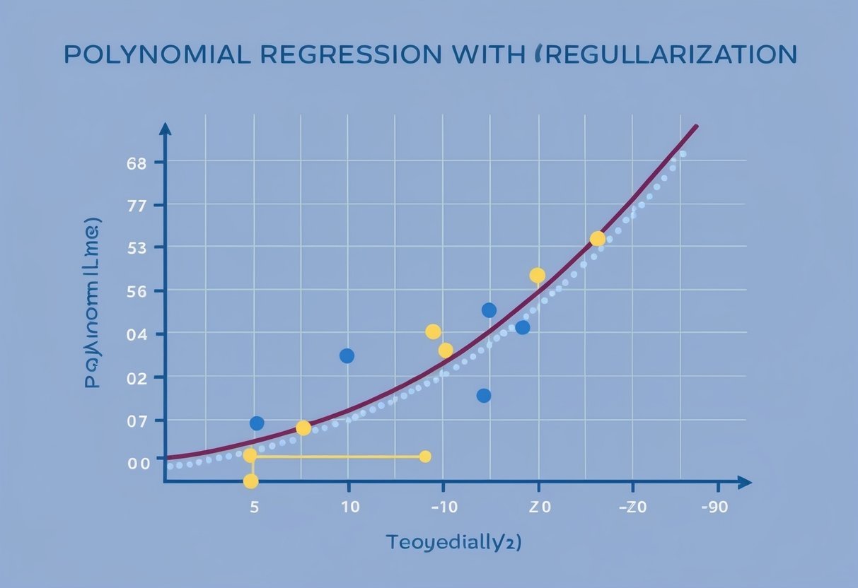
Polynomial regression is an extension of linear regression used to model data with a non-linear relationship. Unlike simple linear models, polynomial regression can capture curvatures in data by including polynomial terms such as squares or cubes of the predictors.

This approach still uses the method of least squares to minimize errors but allows for a more flexible fit to complex datasets.

For example, a quadratic model (including squared terms) can curve a line to better match the data points. This technique is particularly useful when linear relationships are insufficient.

Care must be taken to select the correct degree of the polynomial, as a higher degree can lead to overfitting, making the model less generalizable.

Leveraging Regularization Methods

Regularization methods can reduce overfitting by adding penalties to the regression model’s complexity.

Common techniques include Lasso and Ridge regression, which modify the cost function used in least squares to balance the model fit and its complexity.

Lasso (L1 regularization) tends to produce sparse models by shrinking some coefficients to zero, effectively selecting relevant features.

Ridge (L2 regularization) shrinks coefficients but retains all features, which can stabilize the solution for datasets with multicollinearity.

Both approaches help in creating models that generalize better to unseen data by preventing overly complex models that fit the noise in the training set.

Using these methods ensures that the model retains necessary features while avoiding the pitfalls of overfitting, making it robust and reliable for predictions.

Measuring Regression Accuracy

Understanding how well a regression model makes predictions is crucial. This involves analyzing the model’s residuals and error metrics like MAE, MSE, and R-Squared.

Fine-tuning the model ensures more accurate predictions.

Residuals and The Importance of Fit

Residuals are the differences between actual and predicted values. They indicate how well the regression line fits the data.

A good fit implies that residuals are randomly distributed around zero. When residuals show a pattern, it suggests the model could be improved.

Plotting residuals helps identify any patterns. Consistent patterns in residuals often indicate that the model is missing key relationships.

Thus, analyzing residuals is essential to determine if adjustments are needed to improve the model’s accuracy.

Error Metrics: MAE, MSE, and R-Squared

Mean Absolute Error (MAE) measures the average magnitude of errors in predictions, ignoring their direction. It’s calculated as the average of the absolute differences between predicted and actual values.

Mean Squared Error (MSE) considers both variance and bias, making it useful for sensitive datasets. It squares each error, so larger errors have more impact.

R-Squared, or the coefficient of determination, indicates how well data points fit a model. It’s a measure of explained variance, and its value ranges from 0 to 1. An R-Squared close to 1 means predictions are more accurate.

These metrics are key to evaluating model performance and guiding improvements.

Fine-Tuning Predictions

Improving predictions often involves tweaking model parameters. Techniques like cross-validation and grid search can help refine models.

Cross-validation involves dividing the dataset and testing the model on different subsets, ensuring robustness. This process helps identify the best fitting parameters.

Another approach is to adjust model complexity. This involves finding a balance between underfitting and overfitting.

Adding relevant features, transforming variables, or using regularization methods can enhance predictions.

Fine-tuning maximizes accuracy by finding the most effective model configuration.

Frequently Asked Questions

Linear regression is a crucial topic for those interested in data analysis and machine learning. Understanding how to implement it in Python can help analyze relationships between variables effectively. Here are some frequently asked questions to guide new learners.

How do you perform linear regression analysis using a specific dataset in Python?

To perform linear regression on a dataset, one first needs to explore the data using libraries like pandas for data manipulation. Then, tools such as scikit-learn or statsmodels can be applied to fit a linear model.

These libraries offer functions that simplify fitting and evaluating regression models.

What are the necessary steps to implement linear regression from scratch in Python?

Implementing linear regression from scratch involves several steps. First, clean and prepare the data. Then, calculate the line of best fit that minimizes error by using the least squares method.

Once the model is defined, predictions can be made. Resources like Analytics Vidhya offer detailed guides on this process.

Which Python libraries are considered best for conducting linear regression analysis?

Python offers several robust libraries for linear regression. Common options include scikit-learn for its ease of use and efficiency, and statsmodels for detailed statistical insights.

NumPy and pandas are also helpful for data manipulation and preparation.

Can you provide an example of how to build and interpret a multiple linear regression model in Python?

To build a multiple linear regression model, scikit-learn can be used. Begin by importing the necessary libraries and dataset. Then, separate the dependent and independent variables.

Use the model’s coefficients to interpret the relationship between variables. GeeksforGeeks provides practical examples.

How is the pandas library utilized for linear regression tasks in Python?

Pandas is instrumental in preparing and cleaning data for linear regression. It allows users to handle missing values, normalize data, and create data frames needed for regression models.

The library is often used alongside others like scikit-learn to manage data pre-processing efficiently.

What are the core concepts one must understand when learning about linear regression in the context of machine learning?

Key concepts in linear regression include understanding the relationship between dependent and independent variables. Also, the significance of the slope and intercept, and how these elements influence predictions.

Learners should also grasp how to evaluate a model’s accuracy through metrics like R-squared. These foundational ideas are essential for effective model interpretation.

Understanding SQL Views

SQL views are a key feature in relational databases. They act as virtual tables that present data from one or more tables through a stored query.

Views make complex queries manageable and enhance data security.

Definition and Purpose of Views

A view in SQL is a virtual table that fetches data from one or more underlying tables. Unlike traditional tables, a view does not store data. Instead, it runs a stored SQL query each time it is accessed.

The primary purpose of views is to simplify complex SQL queries. They allow users to focus on the specific data they need without diving into the complexity of the database structure.

This helps in maintaining data security by restricting user access to specific data points without exposing the entire database architecture.

By using views, database administrators can control the visibility of data. It ensures users only see the information relevant to their needs, enhancing both security and performance.

Views are valuable in creating dynamic and efficient data retrieval mechanisms.

View Types: Simple vs. Complex

Views can be classified into two main types: simple and complex.

A simple view is based on a single table and does not involve any functions or groupings. These views are straightforward and easy to update.

On the other hand, complex views involve multiple tables, functions, or groupings. They are used for advanced data manipulation and reporting tasks.

Complex views often include JOIN operations or aggregate functions, making them suitable for report generation and data analysis.

While simple views are easier to manage and update, complex views provide flexibility and power for users needing deep insights into the data. Understanding when to use each type depends on the requirements of the task at hand, balancing simplicity with functionality.

Creating SQL Views

SQL views are essential tools for organizing data from one or more base tables into a virtual table. They streamline complex queries and enhance data security by controlling access to the underlying data.

Below are key aspects of creating SQL views and managing them effectively.

Basic Create View Syntax

The CREATE VIEW statement is used to define a new SQL view. A view is a virtual table created from the result of a SELECT statement. This means it does not store data itself but presents data dynamically from the underlying tables.

To write a basic create view statement, you need to define the view name, followed by the SELECT statement that specifies the data to be included. The syntax generally looks like this:

CREATE VIEW view_name AS
SELECT column1, column2, ...
FROM table_name
WHERE condition;

This structure helps simplify large and complex queries by encapsulating them into a view with a simple name.

Using a view, users can query data as if it were coming from a regular table, without getting into the complexities of the underlying tables and joins.

Create Or Replace View

The CREATE OR REPLACE VIEW command is useful when a modification to an existing view is needed. This command allows a view to be updated without first dropping it.

When working with SQL Views, the need to update query logic frequently arises. Using the CREATE OR REPLACE VIEW statement ensures that these changes can be implemented seamlessly. An example of this command in SQL would be:

CREATE OR REPLACE VIEW view_name AS
SELECT column1, column2
FROM table_name
WHERE new_condition;

This functionality is especially helpful in environments where dependencies exist on the view and dropping it is not an option. It maintains the consistency of queries while allowing for flexibility in data presentation.

The ability to replace views simplifies maintaining and updating application logic, as it ensures that the views remain up-to-date with the most current data requirements.

Querying Through Views

When using SQL views, querying data becomes more efficient and organized. Views act as virtual tables, allowing users to access complex data sets with ease. They simplify the process by letting users focus on what they need without dealing with complex underlying queries.

Running Select Statements

To access data using a view, a SELECT statement is used. This allows users to retrieve data from the view as if it were a regular table.

For example, to get employee names and departments, one might write:

SELECT name, department FROM employee_view;

Filters can also be applied. A WHERE clause helps narrow down results. For instance, filtering employees by department would look like:

SELECT name FROM employee_view WHERE department = 'HR';

Using views also enhances security. Users can see only the data they need, without modifying the data itself.

This way, sensitive information is protected while still being accessible through specific queries.

By maintaining a consistent and understandable format, views ensure that complex data retrieval tasks are performed effectively and securely. This makes it easier for teams to manage and query their data without compromising on efficiency.

Modifying Data Using Views

When working with SQL views, users can perform operations like inserting, updating, and deleting data. These actions allow for managing data within the view while preserving the underlying table structure.

It’s essential to understand how each operation works and their limitations.

Insert, Update, and Delete Operations

Inserting, updating, and deleting data through views involve specific SQL statements.

Users can perform insert operations with caution because inserting is possible only if the view references columns directly from a table without computations or aggregations.

For updates, the UPDATE statement lets users change the view’s data. However, this is only applicable if the view allows updates.

Using the WITH CHECK OPTION ensures that modified data remains consistent with the view’s conditions.

Deleting data involves the DELETE statement. This action removes records, provided that the view includes rows from a single table.

All these operations must adhere to SQL permissions and view conditions to execute successfully.

It is important to remember that not all views support these operations due to structural or permission constraints.

Managing View Security

SQL views play a crucial role in managing data access and security by allowing users to interact with database content without direct table access. This approach enables administrators to control who can view or modify data, ensuring protection against unauthorized access.

Controlling Access to Data

Views allow database administrators to set up security by limiting access to the underlying tables. Through views, specific columns or rows can be hidden, allowing only authorized users to access sensitive data.

This is often achieved by creating views that only include the necessary data, thus reducing exposure.

To further enhance security, views can be combined with user permissions and roles. Only users with the correct permissions can execute queries on these views, adding an extra layer of protection.

For example, a view might show only anonymized data to general users, but full data to managers.

By setting up roles and permissions, one can ensure that sensitive data stays secure while still being accessible to those who need it.

For more detailed guidance, you can learn how to use views in SQL Server to manage data securely.

Performance and Optimization

Optimizing SQL views can significantly enhance the performance of complex queries. It’s important to understand how views can impact query execution and data consistency.

Views Impact on Query Performance

Views can serve as a powerful tool for simplifying complex queries. They allow users to save the structure of a query, which can then be reused multiple times.

This can improve performance, as the database management system may optimize the execution plan by using stored results.

Tools like the SQL Server Query Optimizer can be useful in this context.

However, if not properly indexed, views may also slow down performance. This is especially true if a view is built on other views or complex queries.

Indexed views, or materialized views, can address these issues by storing query results, thus reducing execution time.

It’s important to continuously monitor and tune views to ensure they provide consistent and efficient query performance.

Effective view optimization must balance speed with maintaining data consistency, ensuring that data retrieval remains accurate and reliable.

Dropping SQL Views

Dropping a view in SQL involves removing the view’s definition and any associated permissions from the database. This process requires using specific SQL commands to ensure accuracy.

Correctly Removing Views

To delete a view, the DROP VIEW statement is used. This command precisely targets the view that needs to be removed.

For example, if a view named “CustomerView” is no longer needed, the execution of DROP VIEW CustomerView; will delete it.

It’s crucial for database administrators to ensure that the correct view is specified, as this process is irreversible.

When a view is dropped, its definition and all related permissions are removed from the system catalog.

Multiple views can be dropped at once by separating them with commas in one command as shown in resources like Microsoft Learn.

Understanding the implications of deleting a view is important. This action might affect other database processes or applications that rely on the view.

Therefore, checking dependencies before dropping a view is recommended to avoid unintended disruptions.

Altering Existing Views

Altering views in SQL involves modifying the view definition, allowing users to update how data is presented without altering the original tables. The process relies on the ALTER VIEW statement, which defines the new structure of the view.

Changing View Structure

The ALTER VIEW statement is essential for updating a view. It allows for changes such as adjusting which columns are selected or altering conditions to refine data.

The basic syntax looks like this:

ALTER VIEW view_name AS 
SELECT columns 
FROM tables 
WHERE conditions;

When a view is altered, all indexes on an indexed view are dropped. This means indexed views will automatically lose their indexes after modification.

Re-indexing is necessary if you need to maintain certain index optimizations.

Users need appropriate permissions to alter a view, namely ALTER permission on the object. This ensures that only authorized users can modify existing views, maintaining database integrity.

More detailed instructions are available in the ALTER VIEW Documentation.

Understanding Joins in Views

SQL Views can integrate data from multiple tables, making them powerful for reporting and analysis. By incorporating joins, you can combine this data dynamically, ensuring a comprehensive view without duplicating efforts or data.

Incorporating Joins in View Definitions

When creating a SQL View, using joins allows you to pull related data together seamlessly.

The INNER JOIN is commonly used in view definitions to ensure only matching records from related tables are included.

For instance, linking an EmployeeView with a Departments table can provide a complete list of employees and their departments.

Defining a view with a join involves specifying the join condition, which links columns from different tables.

Consider the table definitions and relationships involved to maintain data integrity.

The choice of join type, such as LEFT JOIN or FULL OUTER JOIN, affects the results returned by the view.

Using these joins appropriately ensures that the view presents a complete and accurate dataset.

Clear definition and understanding of table relationships are critical.

Each type of join offers unique advantages depending on the desired outcome, with INNER JOIN being straightforward and favored when matching is assured across tables.

Applying these joins correctly is essential for creating effective and resourceful SQL Views.

SQL Server-Specific View Features

SQL Server offers unique features for views that enhance data management and security.

These features help simplify complex queries and protect sensitive information by using views as a layer between users and the actual database tables.

Exclusive View Functionality in SQL Server

SQL Server provides several exclusive functionalities when working with views.

One important aspect is partitioned views, which allow the data to appear as if it comes from a single table even though it might be split across different tables.

Local partitioned views can join tables within the same instance, which is especially useful for organizing large datasets.

Learn more about partitioned views on the Microsoft documentation for Views – SQL Server.

System views in SQL Server let users access catalog metadata, giving insights into database structure and configuration.

These views make it easier to perform data analysis by providing necessary information about SQL Server instances and associated objects.

The integration of system views helps streamline the process of managing database environments efficiently.

Exploring these capabilities can enhance the way organizations handle information within SQL Server environments.

Working with the Database Catalog

The database catalog is a crucial part of managing relational databases. It contains metadata about database objects, making it essential for understanding the structure and organization of the database.

SQL Views play a significant role in this, as they allow users to retrieve specific data from the catalog efficiently.

Listing and Analyzing Views in the Catalog

To work effectively with relational databases, it’s important to list and analyze the views in the database catalog.

SQL Server provides system catalog views like sys.objects and sys.tables to help users access information about the database objects.

The sys.tables view, for instance, includes all the columns relevant to tables.

Using SQL queries, one can list all views by querying catalog views such as sys.views. This returns data defining the properties and structure of views without needing to inspect each view individually.

Queries for specific information about a view can help optimize database performance and usage.

Understanding catalog views helps in maintaining and updating relational databases. It enables admins and users to manage data efficiently, reducing redundancy and increasing accuracy.

By using views, one can simplify complex queries, making data retrieval easier and more efficient.

Complex Query Building with Views

SQL views are powerful tools for managing complex queries. They allow users to simplify the process of handling intricate SQL queries by providing a virtual table that can represent the data needed for a result set.

Views can also enhance security and streamline data access.

Utilizing Views to Simplify Complex SQL

Views are essential for simplifying complex SQL queries.

By creating views, a user can encapsulate complex joins or unions into a single, reusable component. This is especially useful when dealing with complex queries that require frequent access to calculated fields or aggregated data.

Views act as predefined queries stored in the database, which fetch data dynamically.

Users can join a view with other tables or combine multiple views using a union to create sophisticated result sets.

By doing this, users can prevent repetitive query writing, thereby making the development process more efficient.

Furthermore, using views can improve database security.

They can restrict user access to specific columns and rows within a table by abstracting the underlying data structure. This allows users to interact with only the necessary data without exposing sensitive information.

In essence, views serve as an intermediary, allowing users to execute complex queries with ease and safety.

Frequently Asked Questions

SQL views are important for managing and organizing data efficiently. They provide ways to simplify complex queries, ensure data security, and improve performance. Understanding how to create and use views effectively can enhance database operations.

What is the definition of a view in SQL?

A view in SQL is a virtual table that presents data from one or more base tables. It doesn’t store the data itself; instead, it fetches data as specified in the defined query. This makes views a powerful tool for simplifying data access and ensuring consistent results.

What are the different types of views in SQL?

SQL features several types of views, including simple views and complex views. Simple views are based on a single table without grouping or functions, while complex views can involve multiple tables and functions, allowing for more advanced data manipulation and presentation.

How do you create a view in SQL?

To create a view in SQL, use the CREATE VIEW statement followed by the view name and the AS keyword with a select query. For example, CREATE VIEW view_name AS SELECT column_name FROM table_name WHERE condition;. This query defines what data the view will show.

What are the advantages of using views in SQL databases?

Views offer multiple benefits, such as simplifying complex queries and providing a layer of security by restricting data access. They can also improve performance by storing complex query logic in a reusable format and ensuring consistent data calculations across different parts of an application.

How do materialized views differ from standard views in SQL?

Materialized views differ from standard views because they store the data physically rather than just the query. They are typically used to improve query performance by pre-computing and storing aggregated or complex data, reducing the need to recompute large datasets frequently.

Why might one use views instead of tables in SQL?

Views can be used instead of tables to abstract the complexity of underlying database schemas.

They allow users to interact with a simplified representation of the data, making it easier to manage without needing to deal with the actual structure of physical tables.

Views also help enforce data security and privacy by limiting data exposure.

Data Analysis Expressions, or DAX, is a powerful language used in tools like Power BI and Microsoft Excel to create custom calculations and analyze data.

This article will explore key concepts related to DAX, focusing on the creation and use of key measures within data models.

Mastering DAX enables users to perform detailed data analysis, turning raw data into actionable insights. With tools like Power BI, understanding DAX can enhance reports and dashboards, offering a more in-depth look at business metrics and trends.

1) Using CALCULATE for Contextual Filters

The CALCULATE function in DAX is a powerful tool used to adjust the filter context of an expression.

It allows users to manipulate data by changing the conditions under which calculations occur. This flexibility makes it an essential feature for dynamic data analysis.

When using CALCULATE, you can define specific conditions to focus on certain aspects of the dataset. For example, if there is a need to view sales data from a particular year, CALCULATE can be used to apply that filter.

This function changes the existing filter context by adding new ones or altering current conditions.

A unique aspect of CALCULATE is its ability to perform what’s known as a context transition. This means it can transform row context into filter context, making it possible to evaluate expressions within row contexts as if they have been filtered.

To utilize CALCULATE effectively, it’s important to understand how it interacts with other DAX functions.

It can be combined with functions like FILTER to apply more complex conditions. For instance, using CALCULATE with a FILTER function allows for intricate filtering that a simple Boolean expression might not capture.

It’s also noteworthy that CALCULATE can work with table functions. When combined with functions such as SUMX, it enables calculations across subsets of data that meet specific criteria, offering deeper insights into complex datasets.

By mastering CALCULATE, analysts can derive meaningful insights tailored to their business needs.

2) Applying ALL to Remove Filters

The ALL function in DAX is used to remove filters from a table or column. This can help when you need to see overall data without any filtering.

When using ALL on a table, it ignores any slicer or manual filters applied. This gives a full view of the data, allowing comparisons without limitations set by specific filters.

For instance, if there are slicers set for “Country” and “Color,” using ALL will display total sales without these slicers affecting the output.

This is useful when creating measures like “Total Sales ALL” where the aim is to show total numbers irrespective of filter settings. More about this application can be found in the article about using ALL and REMOVEFILTERS DAX functions.

Using the ALL function on specific columns can be beneficial too. It removes context filters from certain columns while keeping others intact, giving more control over which parts of the data are fully visible.

This technique is handy when multiple filters are necessary for a detailed analysis but one specific area needs to be filter-free.

3) Creating Dynamic Measures with SWITCH

Creating dynamic measures in Power BI can help make reports more interactive and customizable. The SWITCH function in DAX is a useful tool for this purpose. It allows you to create measures that change their values based on user input.

To start, a custom table is often created, listing all potential measures. This table serves as the basis for users to select from. The SWITCH function then references this table to dynamically display different values.

Using a slicer, users can choose which measure they want to view. The SELECTEDVALUE function in DAX retrieves the selected measure name from the slicer.

This selected value is used in the SWITCH function to determine which measure to display.

As the user interacts with the slicer, the dashboard updates to reflect their choice. This approach is flexible and enhances user engagement by allowing easy exploration of data without multiple static charts.

This method is used in many Power BI reports to allow seamless switching between measures, giving users control over the data they see.

The tools involved, like the SWITCH and SELECTEDVALUE functions, are a staple in creating dynamic and interactive reports. By using these functions, report creators can provide a more tailored experience for their audience.

For more detailed steps on how to create such dynamic measures, resources like How to Create Dynamic Measures in Power BI Using Slicers offer insights and examples.

4) Utilizing SUMX for Iterative Calculations

SUMX is a powerful function in DAX used for iterative calculations. It operates by evaluating an expression on each row of a specified table. This function is particularly useful when calculations depend on row context, making it ideal for tasks like calculating totals based on complex formulas.

The SUMX function requires two arguments. The first is the table over which it will iterate, and the second is the expression to evaluate for each row. For example, a calculation might involve multiplying column values from each row and then summing the results.

In Power BI, using SUMX allows for detailed insights. It respects both the filter context and the row context, making it versatile.

SUMX can handle complex scenarios where simple aggregation functions like SUM would fall short.

When SUMX is employed, context transition plays a critical role. This refers to changes between row context and filter context. The use of measures within SUMX can lead to context transition, affecting how data is evaluated and displayed.

Understanding this behavior is key to effectively using SUMX for calculations that depend on dynamic contexts.

Performance is an important consideration when using SUMX. It processes each row individually, which can be resource-intensive for large datasets.

Optimizing queries and ensuring efficient data models can help maintain performance while utilizing SUMX capabilities.

Practical applications of SUMX include calculating profitability analyses and custom sales metrics. For example, applying SUMX to compute profits by iterating over sales data can provide deep insights into business performance.

This function is crucial for those who need precise data manipulation in Power BI, leveraging its iterative strength for complex data scenarios.

5) Employing RELATED for Table Relationships

The RELATED function in DAX is essential for creating connections between tables. It retrieves values from another table based on existing relationships. This function is particularly useful when working with data models where tables are connected through many-to-one relationships.

Each time RELATED is used, it accesses the related table’s data, allowing users to pull in necessary information for calculations or reporting purposes. This can streamline data analysis and enhance the understanding of linked datasets.

In practice, RELATED helps with joining tables on shared keys. For example, if a sales table and a product table share a product ID, RELATED can access product details from the sales table.

This ability simplifies the process of including comprehensive data from related tables in reports.

When modeling data, RELATED provides flexibility. It allows users to build more complex models by accessing data across tables.

This capability supports more detailed analyses and can be combined with other DAX functions for even more powerful insights.

Overall, utilizing RELATED in DAX enhances the ability to manage and analyze data across different tables. It plays a crucial role in leveraging relationships within a data model, making it a key tool for anyone working with DAX and Power BI.

For more information, you can explore how RELATED works within the context of row iteration on SQLBI’s article about RELATED in DAX.

6) Optimizing Performance with Variables

Using variables in DAX calculations can greatly enhance performance. When writing DAX formulas, variables allow for storing intermediate results. This reduces the number of calculations needed, which means faster queries and potentially lower resource usage.

Variables help improve the readability of DAX expressions. They allow for assigning meaningful names to parts of a formula, making it easier to understand and maintain.

By storing these parts in variables, DAX code becomes clearer and more approachable.

Debugging also becomes simpler with variables. When a formula does not produce the expected result, having variables can make it easier to identify and fix problems.

Changes can be made to variables without altering the whole structure, simplifying the troubleshooting process.

Variables in DAX are local, which means they exist only within the context of a single formula. This allows for precise control over calculations, as variables do not interfere with other parts of the DAX model.

This local nature distinguishes them from measures, which are global and can be reused across different calculations.

Writing efficient DAX code can reduce potential bottlenecks. For example, if multiple measures aggregate the same column differently, this can slow down performance.

Variables can mitigate these issues by streamlining calculations and minimizing redundancy.

7) Leveraging HASONEVALUE for Unique Conditions

In DAX, the HASONEVALUE function helps when making sure a calculation is based on a single item. This is useful when a measure should only be calculated if there is one unique value visible in the filter context.

Using HASONEVALUE, users can return specific results or messages if there are multiple selections. For example, in a sales report, a measure might show average sales only if one product is selected.

If more than one product is chosen, it can display a message indicating ambiguity.

Another key use of HASONEVALUE is in handling hierarchical data. When working with categories and subcategories, it ensures ranks or calculations apply at the correct level. This prevents errors when data is grouped or filtered by different levels.

HASONEVALUE is also valuable when comparing results across different slices of data. For instance, comparing sales years requires knowing if the data is filtered by one specific year.

This ensures meaningful and accurate comparisons.

These versatile applications highlight the importance of understanding filter contexts in Power BI and other DAX environments. By leveraging HASONEVALUE effectively, users can ensure their reports and dashboards are both accurate and informative. This results in clearer insights and more actionable data.

8) Incorporating USERELATIONSHIP for Inactive Relationships

When working with DAX, managing relationships between tables is crucial. Sometimes, a model includes more than one relationship between tables, but only one can be active at a time. This is where the USERELATIONSHIP function becomes valuable.

USERELATIONSHIP allows users to specify which relationship to use when evaluating an expression. This is particularly useful when dealing with inactive relationships.

In an inactive relationship, the connection between tables is defined, but not used automatically in calculations.

For example, if a table has relationships through both a sales date and a delivery date, only one can be active by default. To use the inactive relationship when needed, one can apply USERELATIONSHIP in a DAX expression. This ensures the correct data context is applied for the calculation.

Using USERELATIONSHIP in DAX does not affect the active status of relationships permanently. It only applies the specified relationship when the DAX query is executed. This function enables flexibility in data modeling, allowing users to leverage all available relationships effectively.

Incorporating USERELATIONSHIP is straightforward. By naming the two columns that define the relationship in question, it’s possible to override the active relationship temporarily.

This targeted use of relationships can enhance data accuracy and insights, especially in complex data models.

9) Designing Time Intelligence with DATESYTD

The DATESYTD function offers a straightforward way to handle year-to-date calculations in DAX. It generates a table with all the dates from the beginning of the year up to a specified date, making it valuable for time-sensitive data analysis.

Using this function can simplify the process of analyzing sales or revenue data on a yearly basis. By applying DATESYTD, one can easily compare the current year’s performance against previous periods, helping identify trends and make informed decisions.

To make use of DATESYTD, the data model must have a proper date table established. This ensures calculations return accurate and meaningful results.

A well-formed date table includes continuous dates without gaps, which is crucial for the function to operate effectively.

Another key aspect of using DATESYTD is integrating it with the CALCULATE function. This combination allows for manipulating and filtering data, providing more detailed insights into the yearly trends and patterns that might otherwise go unnoticed.

In Power BI, adding a measure with the DATESYTD function can enhance visualizations. It allows users to create dynamic reports that automatically update as new data is added, aiding in real-time decision-making.

Moreover, visual tools like this can help users understand data better without delving into complex analysis methods.

10) Implementing Custom Aggregations Using AVERAGEX

The AVERAGEX function is a powerful tool in DAX that performs custom aggregations on data sets. It evaluates an expression for each row in a table and calculates the arithmetic mean of the results. This allows users to create complex calculations beyond standard averages.

In AVERAGEX, the first argument specifies the table to work with. This can be a physical or a virtual table, providing flexibility in data analysis. The AVERAGEX function works by running a given expression over each row, resulting in a set of values that it averages.

Using AVERAGEX can simplify complex data scenarios. For instance, in analyzing energy consumption trends, AVERAGEX can be used alongside the FILTER function to create subsets of data, helping highlight changes in patterns effectively. Unlike simpler measures, AVERAGEX provides a more nuanced view of the data by focusing on calculated expressions.

The function is part of iterative functions like SUMX in DAX, allowing users to perform detailed analytical tasks.

Users can analyze how using virtual tables within AVERAGEX can explore and manipulate data dynamically. This feature makes it a valuable tool when working with relational data models, such as those in Power BI.

When creating custom aggregations, having an understanding of how to specify expressions and table arguments is essential. This knowledge enables more tailored and specific data insights, enhancing overall data analysis capabilities.

Understanding DAX Language

Data Analysis Expressions (DAX) is a powerful language used in Power BI, Power Pivot, and SQL Server Analysis Services. It provides versatile tools to perform calculations and manage data. It is essential to understand both its syntax and functions to effectively use DAX.

Basics of DAX Syntax

DAX syntax resembles Excel formulas but operates in a relational data model. This means it is designed to work effectively with tables and columns.

Each DAX expression starts with an equals sign = and uses functions, operators, and values to perform calculations.

For example, the syntax SUM(Sales[SalesAmount]) calculates the total of the SalesAmount column in the Sales table. It’s crucial to know how to reference tables and columns properly since they are the primary components in DAX expressions. Brackets [] are used around column names, while table names are usually referenced directly.

Understanding these basic elements allows users to construct meaningful calculations and analyses.

Common DAX Functions

DAX functions are an integral part of crafting expressions in the language. They include mathematical, text, logical, and time intelligence functions, among others.

Some widely used functions are SUM, AVERAGE, and FILTER.

SUM helps in adding up number values in a column, while FILTER returns a table that contains only rows with desired conditions.

Time intelligence functions, such as TOTALYTD, PREVIOUSMONTH, and more, allow for analyzing data over time periods.

Mastering these functions is essential for developing advanced data models and performing sophisticated data analysis. These functions enhance the capabilities of DAX, facilitating a deeper insight into data sets.

Key Measures Table Concepts

Key measures tables are crucial in analyzing data effectively. They help in summarizing large sets of data while providing insights into business intelligence. These tables are optimized for use in powerful tools like Power BI.

Importance of Key Measures

Key measures tables allow users to efficiently manage and organize various metrics. By creating a dedicated table for measures, data professionals can streamline their data models. This organization aids in maintaining clarity and avoiding clutter in data fields, making it easier to access and interpret data.

They help in separating calculated measures from raw data to simplify model navigation.

Moreover, these tables enable easier documentation and sharing of data models within teams. By maintaining a clear structure, both current and future team members can identify and utilize the critical metrics needed for their analyses without confusion.

Application in Business Intelligence

In business intelligence, key measures play a pivotal role in driving data-driven decisions. With tools like Power BI, users can leverage these measures to create dynamic reports and dashboards. These enable companies to track performance, forecast trends, and make informed decisions quickly.

By organizing key measures effectively, businesses can ensure their analytics are accurate and accessible. This organization helps in comparing different metrics, providing a holistic view of company performance.

Utilizing measure tables in Power BI can enhance the user’s ability to adjust to changing analysis needs, supporting agile decision-making processes. Adding filters or slicing data is more intuitive, which enhances data storytelling.

Advanced Techniques in DAX

In mastering DAX, focusing on advanced techniques is crucial. This involves optimizing performance and addressing common troubleshooting scenarios. Exploring these areas can significantly enhance data analysis skills and efficiency.

Optimizing Performance

Performance optimization in DAX involves various strategies. One key approach is handling large datasets efficiently. By using calculated columns sparingly, the performance can be improved.

Calculated measures are often more efficient than columns because they are evaluated only when needed.

Using the right functions also plays a role. Functions like SUMX and FILTER can be resource-intensive. Instead, using functions like CALCULATE and SUM when possible can reduce processing time significantly.

Another important aspect is using variables to store intermediate calculations, lowering the number of calculations performed repeatedly.

Managing relationships in data models is essential too. Ensuring that relationships are set up optimally helps in minimizing the calculation time needed by DAX formulas.

Indexes and data model design choices can directly impact calculation speed and performance.

Troubleshooting Techniques

Troubleshooting DAX calculations often requires checking for common errors. One frequent issue is incorrect use of context, especially row context and filter context. Understanding how these contexts affect calculations can solve many errors.

When a formula does not return expected results, reviewing the logic in DAX expressions is crucial. Looking for misplaced or unnecessary functions can help pinpoint the issue.

Using built-in tools like the Performance Analyzer in Power BI can help identify bottlenecks in calculations.

Another approach is using debugging tools to trace errors. Techniques like breaking down complex DAX formulas into smaller parts can make finding errors easier. By testing these smaller parts individually, one can often identify faulty sections quickly.

Frequently Asked Questions

This section covers important queries related to creating and using tables of measures in DAX, practical examples, learning strategies, and recommended resources. These insights will assist individuals in enhancing their DAX skills effectively.

How can I create a table from measures in DAX?

Creating a table from measures involves defining measures with DAX expressions. These measures can then be organized in a Power BI report or a PowerPivot model. Utilizing functions like CALCULATE and ALL can help tailor the calculations to specific needs.

What are some common examples of measures in DAX?

Common measures in DAX include calculations like total sales, average revenue, or count of customers. These measures often use functions such as SUMX, AVERAGE, and COUNTX. They are essential for generating insights in data models.

Where can I find a comprehensive list of DAX functions for use in Power BI?

A comprehensive list of DAX functions is available on Microsoft’s official Power BI documentation. It provides details and examples for each function, aiding users in understanding their applications.

What are the best practices for learning DAX efficiently?

Best practices include starting with foundational functions like RELATED for managing table relationships and gradually advancing to more complex ones like SWITCH for dynamic measures. Regular practice and solving practical problems can accelerate learning.

What resources are recommended for beginners to learn DAX?

Beginners can benefit from guides like Getting Started with DAX in Power BI, which offers step-by-step instructions. Online courses, community forums, and video tutorials are also useful resources for learning.

How can I understand the use of the ‘table’ function in DAX?

The ‘table’ function in DAX is crucial for managing data within a specified context.

It is often used to create filtered datasets or join tables for analysis.

Understanding table functions involves practice with data contexts and using examples from comprehensive guides.

Understanding Database Normalization

Database Normalization is the process of organizing data to reduce redundancy and improve data integrity.

This involves dividing large tables into smaller, manageable pieces without losing meaningful connections between the data.

There are several normal forms used to structure databases. The main goal is to make data storage more efficient and reliable.

First Normal Form (1NF) ensures each column contains atomic values, meaning they are indivisible. This helps prevent repeat data within a table.

Second Normal Form (2NF) builds on 1NF by removing subsets of data that apply to multiple rows of a table. Data is placed in separate tables linked with foreign keys.

Third Normal Form (3NF) strives to remove data not dependent on the primary key. This further simplifies the structure by ensuring that only data directly related to a table’s primary key is kept within that table.

The purpose of normalization includes reducing data redundancy and preventing data anomalies during insertions, deletions, and updates.

Normalization in databases like these help maintain consistency and make databases easier to manage. Data is organized logically, making it accessible and streamlined. For more on normal forms, you can refer to resources such as those at Guru99.

Concept of Normal Forms in DBMS

Normal forms in DBMS are crucial for organizing and structuring databases. Each step in normalization removes redundancies and ensures data integrity.

Here, we explore how data is refined through different normal forms: from basic separation to complex structure adjustments.

Defining Normal Forms

Normal forms in database management categorize the structure of tables to minimize redundancy and dependency. First Normal Form (1NF) ensures that each column contains atomic values, promoting unique entries.

Second Normal Form (2NF) builds on 1NF by removing partial dependencies of any column on a primary key. This step involves making sure that each piece of data relies on the table’s unique identifier, thus enhancing data consistency.

As you progress, Third Normal Form (3NF) further refines data by eliminating transitive dependencies. This means that non-prime attributes (those not part of a key) are only dependent on super keys.

Boyce-Codd Normal Form (BCNF) is a stringent version of 3NF, handling anomalies by ensuring every functionally dependent column is a super key.

Advanced forms like Fourth (4NF) and Fifth Normal Forms (5NF) focus on multi-valued dependencies and complex relational structuring, while Sixth Normal Form (6NF), less commonly used, deals with temporal databases.

Importance of Sequential Progression

Adopting normal forms sequentially is essential for systematic data organization.

Starting with 1NF is vital as it lays the groundwork by ensuring atomic values in each field.

Proceeding to 2NF and 3NF reduces redundancies, making data more efficient for queries.

As normalization progresses, each step reduces the chance of anomalies. BCNF ensures stricter conditions, ideal for preventing data discrepancies.

Higher forms like 4NF and 5NF must be considered for databases with intricate data relationships, ensuring detailed dependency management.

Sequential progression ensures that databases are optimized for performance, integrity, and scalability, making them more reliable for extensive data operations.

First Normal Form (1NF)

The First Normal Form (1NF) focuses on making sure that each database table has atomic values and no repeating groups. These criteria help ensure data is efficiently organized, preventing redundancy and enhancing consistency.

Criteria for 1NF

For a table to meet the requirements of the First Normal Form, each field must contain only atomic values. This means that fields should not hold multiple values.

For instance, instead of having a list of phone numbers in one column, each phone number should have its own row.

Each table should have a primary key. This key uniquely identifies each record. No identical rows should be present, ensuring every entry is distinct.

Additionally, each column should only contain values belonging to a single category. For instance, a “Date of Birth” column must not include phone numbers.

These rules aim to reduce data redundancy. Redundancy can lead to inconsistencies and wasted storage space. Ensuring compliance with 1NF helps structure data more logically and efficiently.

Benefits of 1NF

Following the First Normal Form rules provides several advantages.

By using atomic values, databases become easier to search and filter. This results in faster query responses and simpler updates.

1NF also minimizes redundancy. With only unique entries and no repeating data, storage is utilized more effectively, and the risk of errors is reduced.

Maintaining consistency becomes easier, as each change needs only to be made once.

Moreover, implementing 1NF sets a foundation for higher normal forms. It simplifies the progression to more advanced normalization stages, ensuring the database remains organized as complexity increases. This enhances both the performance and reliability of the database system.

Second Normal Form (2NF)

Second Normal Form (2NF) is a crucial step in database normalization. It addresses issues related to partial dependency and ensures that each non-key attribute is entirely dependent on the primary key.

Achieving 2NF

To achieve 2NF, a table must first be in First Normal Form (1NF). This means the table should contain no repeating groups or arrays.

The next step is eliminating partial dependencies.

A table meets 2NF when all non-key columns are fully functionally dependent on the primary key. In simpler terms, non-key attributes should depend fully on the entire primary key, not just a part of it.

This ensures that the data is free from redundancies caused by partial dependencies.

For instance, if a table has a composite primary key, each non-key attribute must depend on both parts of the key. This reduces data duplication and enhances the table’s integrity by making it manageable and consistent.

Partial Dependency Elimination

Partial dependency occurs when a non-key attribute depends on only a part of a composite primary key. In 2NF, this issue must be eliminated to maintain data consistency and avoid unnecessary duplication.

For example, consider a table with a composite primary key of (OrderID, ProductID). If an attribute like ProductName depends only on ProductID but not OrderID, it creates a partial dependency.

To resolve this, create a separate table for ProductName with ProductID as the primary key.

The elimination of partial dependencies helps in organizing databases more efficiently, ensuring that each attribute is stored only once and reducing the risk of anomalies during data updates.

Third Normal Form (3NF) and BCNF

Third Normal Form (3NF) and Boyce-Codd Normal Form (BCNF) focus on eliminating types of dependencies in a database. 3NF deals with transitive dependencies, while BCNF addresses situations where all non-trivial functional dependencies are handled.

Understanding 3NF

Third Normal Form (3NF) is an important step in organizing a database. A relation is in 3NF if it is in Second Normal Form (2NF) and there are no transitive dependencies.

This means no non-prime attribute should depend transitively on the candidate key.

An attribute is considered non-prime if it doesn’t participate in any candidate key of the table. For example, if “CourseID” leads to “CourseName” and “Professor,” with “CourseName” determining “Professor,” then “Professor” is transitively dependent and should be separated.

This ensures that only the primary key determines non-prime attributes, reducing redundancy.

Transition to BCNF

Boyce-Codd Normal Form (BCNF) is a stronger version of 3NF and resolves more complex dependencies. A table is in BCNF if it is in 3NF and every determinant is a super key.

This means any attribute on the right side of a functional dependency should depend only on a super key.

For a relation with a dependency A→B, A must be a super key. For example, if a table has attributes “EmployeeID, Department, Manager,” where “Department” and “Manager” determine each other, this violates BCNF.

Address this by splitting the table into distinct ones that eliminate the dependency problem. By achieving BCNF, databases avoid anomalies better than with just 3NF.

Additional details on normal forms can be found in articles like Difference between 3NF and BCNF and Normal Forms in DBMS.

Advanced Normal Forms

Advanced normal forms in database management focus on reducing redundancy and enhancing data integrity to an optimal level. Fourth and Fifth Normal Forms address complex database anomalies, refining the structure beyond typical normalization needs.

Fourth Normal Form (4NF)

Fourth Normal Form (4NF) is concerned with eliminating multi-valued dependencies in a database. In 4NF, a table should not have more than one multi-valued dependency without a proper primary key linking them. This ensures that the database avoids unnecessary duplication and complexity.

A common example involves a table handling multiple phone numbers and email addresses for each employee. In 4NF, these would be split into separate related tables. Normalization in SQL DBMS helps break these dependencies, maintaining the data integrity and reducing redundancy.

Fifth Normal Form (5NF)

Fifth Normal Form (5NF), also known as Project-Join Normal Form (PJNF), is designed to handle join dependencies. Its focus is to ensure that no information is lost when tables are decomposed into smaller tables that can be joined back together.

A database reaches 5NF when every join dependency is a consequence of the candidate keys.

This form is appropriate for complex databases, where the queries often involve joins of multiple tables. Studytonight’s resource provides insights into how 5NF maintains structural integrity in advanced database systems by addressing complex join dependencies.

Ultimate Normal Forms

Beyond 5NF, the Sixth Normal Form (6NF) exists, though it is rarely used outside of specialized applications. It extends the concept of normalization by focusing on temporal data, ensuring that the database can hold unchanging information over time.

This stage is mainly relevant in certain sectors, such as finance or when dealing with time-series data.

6NF is not commonly implemented in typical database projects but can be vital for high-integrity and time-sensitive information systems. Understanding when to utilize 6NF can be crucial for maintaining historical data accuracy without redundancy, as detailed in discussions on database normalization.

Functional Dependencies and Keys

Functional dependencies and keys play crucial roles in database normalization. Functional dependencies help determine relationships between attributes, while keys ensure uniqueness in database tables.

Understanding Functional Dependencies

A functional dependency occurs when one set of attributes uniquely determines another attribute. For example, if an employee’s ID determines their name, then the name is functionally dependent on the ID.

Functional dependencies help define how attributes relate to one another within a table.

In database design, functional dependencies are used to find candidate keys. A candidate key is a minimal set of attributes that can uniquely identify a row in a table.

Ensuring proper identification of candidate keys is vital for creating a well-structured database. Functional dependencies reveal potential redundancies, guiding optimizations and transformations.

Significance of Keys in Normalization

Keys are essential for database integrity. A primary key is a special candidate key chosen to identify table records uniquely.

It ensures no two rows have the same value and often acts as a reference point for other tables through foreign keys.

A composite key consists of multiple attributes collectively used as a primary key, while a super key is any set of attributes that can uniquely identify rows, potentially beyond what is necessary.

The use of keys, especially primary and foreign keys, is fundamental in normalization to eliminate redundancy and maintain data integrity.

Proper organization of keys ensures that databases remain consistent, enabling accurate data retrieval and manipulation.

Anomalies in Database Tables

Data anomalies occur when data in database tables becomes inconsistent or incorrect. These issues arise from poor database design and can cause problems for data integrity and reliability.

Types of Data Anomalies

Data anomalies are issues that affect the accuracy of data within tables. Common anomalies include insertion, deletion, and update issues.

Insertion anomalies occur when adding new data is not possible without additional, potentially unnecessary data.

For example, adding a new student record might require fictitious data about enrollment if proper relationships aren’t set.

Deletion anomalies happen when removing data unintentionally strips out useful information.

For instance, deleting information about a course could also eradicate all data about the enrolled students.

Update anomalies emerge when modifications in one data point do not synchronize with other related data.

If a student changes their address and this information is not updated everywhere, discrepancies ensue.

Recognizing these anomalies is crucial for maintaining the accuracy and consistency of a database.

Preventing Anomalies through Normal Forms

To effectively manage data anomalies, normal forms are essential. These forms organize and structure database tables to minimize redundancy and dependency issues.

The First Normal Form (1NF) ensures that each table cell holds a single atomic value, and each entry remains unique.

This structure prevents insertion anomalies by maintaining straightforward data entry procedures.

In the Second Normal Form (2NF), all non-key attributes are fully functionally dependent on the primary key.

This setup reduces the risk of update anomalies by linking attributes clearly to a single identifier.

The Third Normal Form (3NF) takes this concept further by ensuring that all attributes depend only on the primary key.

By eliminating transitive dependencies, it reduces deletion anomalies.

Well-defined normal forms contribute significantly to data integrity, minimizing the likelihood of anomalies.

Database Design and Integrity

Database design using normalization techniques aims to organize data efficiently while ensuring data integrity and consistency. The design process focuses on structuring databases to prevent data anomalies.

Designing Databases with Normalization

Normalization is a key aspect of database design that divides large tables into smaller, more manageable ones.

This process reduces redundancy and dependency, which helps maintain data consistency across the system.

It involves organizing data into normal forms, each step refining and improving the structure.

Each normal form has specific rules to be followed. For instance, in the First Normal Form, all table entries must be atomic, with no repeating groups of data.

In the Second Normal Form, data must meet all the criteria of the First Normal Form, and each non-key attribute must depend on the table’s primary key.

Maintaining Data Integrity

Data integrity ensures that information within a database is accurate and reliable.

One crucial aspect is referential integrity, which involves maintaining consistency through relationships between tables. This prevents the entry of invalid data into a database by using foreign keys, ensuring all table references remain accurate.

Integrity constraints protect against unintended data loss or corruption.

Enforcing rules within the database management system ensures that operations align with business logic.

Strategies like transaction management further enhance consistency by treating operations as a single unit, ensuring all steps are completed successfully.

Implementing these measures preserves data quality, safeguarding against errors and aiding in long-term data management.

Normalization and SQL

Normalization in SQL is essential for organizing data efficiently. It involves structuring a database to minimize redundancy and improve data integrity.

By applying normal forms and optimizing SQL queries, databases can support fast, accurate data retrieval.

Applying Normal Forms in SQL

Normalization in SQL consists of several steps, each addressing different issues.

First Normal Form (1NF) requires each table column to hold only one value, eliminating repeating groups.

Second Normal Form (2NF) addresses partial dependency, ensuring every non-key attribute is fully dependent on the primary key.

Third Normal Form (3NF) removes transitive dependencies, where non-key attributes depend on other non-key attributes.

Foreign keys play an important role in this process, linking tables and maintaining referential integrity.

By enforcing relationships between tables, foreign keys help prevent anomalies.

SQL developers must be familiar with these concepts to design robust, scalable databases that support complex applications.

Familiarity with these normal forms is crucial for maintaining data consistency in systems like MySQL.

Writing Efficient SQL Queries

Efficient query writing in SQL is essential for maintaining performance, especially in large databases.

When queries are poorly constructed, they can slow down retrieval times significantly.

To enhance query performance, developers should focus on indexing.

Proper indexing can drastically reduce search times in large datasets, allowing for quicker access to needed data.

Moreover, eliminating unnecessary columns and joining only required tables can streamline SQL queries.

Using SELECT statements that target specific fields rather than retrieving entire tables can optimize operations.

SQL professionals should apply these techniques to ensure efficient data handling, keeping systems responsive and reliable.

Implementing these strategies helps manage data effectively across various platforms, including popular systems like MySQL.

Challenges and Trade-offs in Normalization

Normalization in databases enhances data consistency and reduces redundancy. Yet, achieving the ideal level involves balancing flexibility and database performance. Understanding these aspects helps in making informed design decisions.

Analyzing Normalization Trade-offs

Normalization improves data integrity by organizing data into tables and ensuring dependability. Yet, this process can lead to slower query performance.

Joining several tables for a single query can increase complexity, affecting response time. As a result, designers often face challenges in optimizing performance.

Increased normalization might also reduce flexibility when future data requirements change.

Balancing these factors is key to effective database management.

Understanding how normalization impacts different system aspects helps. This includes evaluating performance bottlenecks and flexibility constraints.

It’s essential to weigh these considerations against potential benefits, such as data integrity and reduced redundancy.

Deciding on the Level of Normalization

Deciding on the appropriate level of normalization depends on various factors like the specific needs of a system.

While first normal form (1NF) eliminates repeating groups and ensures atomic values, higher forms, like third normal form, further delineate data relationships.

Yet, excessive normalization can lead to efficiency losses.

Choosing the correct level impacts how the database handles real-time applications.

While highly normalized databases reduce redundancy, they might not suit environments needing rapid query responses.

It’s important to assess the trade-offs between data redundancy and query speed, tailoring the normalization approach to the system’s demands, balancing both flexibility and performance.

Normalization in Practice

Normalization is a key process in organizing databases to reduce redundancy and improve data integrity. By structuring database tables effectively, normalization helps in efficient data management and facilitates easier database operations.

Real-world Normalization Examples

In many offices, customer databases are normalized to improve efficiency. For instance, a retail store might store customer details like name, address, and purchase history in different tables.

This ensures that updates to customer information are made only once, reducing errors and maintaining consistent data across the system. It simplifies queries by keeping data organized and helps in generating accurate reports.

Another example is in banking systems where transaction details, customer information, and account data need to be managed separately yet efficiently.

By normalizing these databases, banks can quickly retrieve and update specific data without the risk of altering unrelated information. This enhances security and speeds up transaction processes.

Normalization in Database Management Systems

Database Management Systems (DBMS) rely on normalization to maintain data quality.

In a DBMS, normalization involves organizing tables to ensure that they only store data relevant to each other.

For instance, in Database Normalization, tables must comply with rules of First Normal Form (1NF), Second Normal Form (2NF), and Third Normal Form (3NF) to eliminate redundancy.

By applying these rules in DBMSs, the systems reduce data anomalies and improve storage efficiency.

Each table has well-defined relationships, leading to easier maintenance and query optimization. This approach is essential in handling large datasets, ensuring that the information is accurate and easy to access without unnecessary duplication.

Frequently Asked Questions

Normalization in database management organizes data efficiently to minimize redundancy and maintain data integrity. These processes are essential for effective database design.

What is the purpose of normalization in a database management system (DBMS)?

Normalization helps structure data so each piece is stored only once. This reduces redundancy and ensures consistency. It also makes databases more efficient by organizing tables and relationships, supporting data integrity and ease of maintenance.

How does the first normal form (1NF) differ from the second (2NF) and third normal form (3NF)?

The first normal form (1NF) ensures each table cell holds a single value and each record is unique. The second normal form (2NF) adds that all non-key attributes must depend on the whole primary key. Third normal form (3NF) further requires that attributes are independent of non-primary key attributes.

Can you provide examples of tables in 1NF, 2NF, and 3NF?

A table in 1NF might list customer IDs and orders, ensuring each cell has a single value. In 2NF, this table would separate repeated data, like splitting order and customer data into distinct tables. In 3NF, it would also remove transitive dependencies, ensuring that all attributes depend directly on the primary key.

What are the steps involved in normalizing a database to the third normal form?

To reach the third normal form, start with 1NF by eliminating repeating data. Move to 2NF by ensuring each non-primary key attribute is fully dependent on the primary key. Finally, achieve 3NF by removing any dependencies between non-key attributes, ensuring everything is directly related only to the primary key.

How do the different normal forms impact the redundancy and integrity of data in a database?

As a database progresses through normal forms, redundancy is reduced. In 1NF, a table might still hold duplicate data. By 3NF, most redundancy is eliminated, contributing to higher data integrity. This ensures databases are easy to update, reducing the likelihood of inconsistencies.

Why is normalization important for efficient database design and what problems does it solve?

Normalization eliminates redundant data, which saves storage and reduces costs.

It simplifies database maintenance and supports robust data accuracy.

Problems like update anomalies are reduced as changes in data occur in fewer places, thus lowering the chance of inconsistencies.

Smooth and fast databases are crucial for powering today’s applications.

Database optimization is the key to ensuring efficient performance and quick data retrieval. With the right strategies, developers can significantly improve the speed and reliability of database systems.

Effective optimization involves several techniques, such as query rewriting and indexing.

These methods help streamline data processing and reduce server load. By adopting these practices, the performance of database systems can be greatly enhanced, allowing for more efficient operations.

Exploring advanced strategies is essential for meeting different system needs.

Whether handling large volumes of data or ensuring quick access times, these techniques play a vital role. As systems grow and evolve, continuous optimization is necessary to maintain performance.

Key Takeaways

• Database optimization ensures fast data access.
• Techniques like indexing improve database efficiency.
• Continuous strategy updates are vital for performance.

Understanding Database Optimization

Database optimization is essential for ensuring optimal performance and efficiency in data management systems.

Key elements include understanding how databases handle tasks and identifying specific goals that drive optimization processes.

Defining Database Performance

Database performance refers to how well a database accomplishes tasks it’s designed for, such as query execution, data retrieval, and transaction processing.

Efficient query execution is vital in achieving high performance. Query plans, indexing, and memory allocation play significant roles in managing system resources and reducing response times.

Performance is usually measured by metrics like transaction throughput, query response time, and resource utilization.

It’s important to allocate resources like CPU and memory effectively to handle peak loads without negatively affecting other operations. Optimizing these components helps maintain system reliability and user satisfaction.

Goals of Optimization

The primary goals of database optimization are to enhance speed, ensure data integrity, and maximize resource efficiency.

Performance tuning targets aspects such as memory usage, buffer management, and connection handling.

By optimizing resource allocation, databases can manage high-demand processes effectively. This includes methods like indexing improvement, query rewriting, and hardware upgrades.

Enhancing these areas allows databases to operate smoothly, minimizing lag and bottlenecks. Ensuring that databases handle their functions efficiently helps achieve smoother operations.

Frequently Asked Questions

Database optimization involves strategies like indexing, writing efficient SQL queries, and normalization. Partitioning and caching also play essential roles. Below are detailed answers to common questions related to these topics.

How can indexing improve database query performance?

Indexing helps by creating a data structure that makes searching faster.

This reduces the time it takes to retrieve data from tables. Using proper indexes ensures queries do not scan the entire table, which boosts performance significantly. Choosing the right columns for indexing is critical.

What are the best practices for writing efficient SQL queries?

Efficient SQL queries avoid unnecessary operations and use functions smartly.

Limiting the number of columns retrieved and employing conditions to filter data reduces processing. Writing precise joins and avoiding complex calculations directly in queries can also improve execution speed.

How does database normalization contribute to optimization?

Normalization eliminates data redundancy and ensures data integrity.

By organizing data into related tables, it reduces duplicate data storage, which optimizes disk space usage. A well-normalized database often leads to improved query performance, as it breaks down large tables into smaller, manageable ones.

What role does partitioning play in database optimization?

Partitioning divides large tables into smaller, more manageable pieces.

This process can improve query performance by allowing the database to read only relevant partitions, rather than the entire dataset. This not only speeds up queries but also aids in efficient data management and maintenance.

How can query caching be utilized to enhance database performance?

Query caching stores the results of a query for later use.

This reduces the need to rerun queries, saving computational resources. By serving frequently requested data directly from the cache, response times improve. Identifying repeated queries and caching them can lead to noticeable performance gains.

What techniques are used for optimizing complex joins in databases?

Optimizing complex joins involves reducing the amount of data being joined. This can be done by filtering data early in the process with WHERE clauses.

Using indexes on columns involved in joins and ensuring that join conditions are properly defined can also improve the efficiency and speed of complex joins.