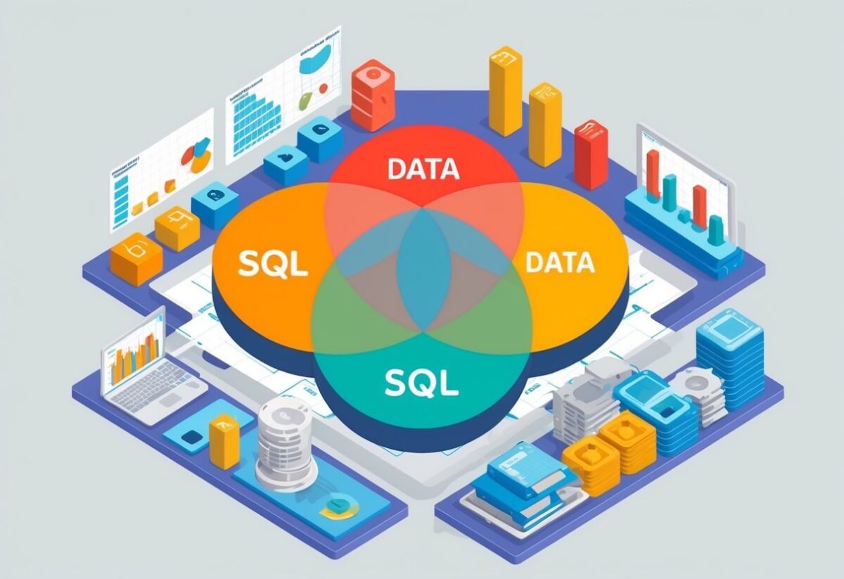
Categories
Uncategorized

Learning What Data Analysis Entails: A Comprehensive Overview

The Fundamentals of Data Analysis

Data analysis serves as a cornerstone for modern decision-making. Understanding it involves grasping key concepts and recognizing its role in shaping data-driven decisions.

Defining Data Analysis

Data analysis is the process of inspecting, cleaning, and modeling data to draw meaningful conclusions. It involves various techniques to transform raw data into useful insights. These insights help organizations make more informed choices.

Analysts often use statistical tools and software to perform these tasks efficiently.

A key part of this is understanding math and statistics. Courses like Fundamentals of Data Analysis on Coursera cover these essentials. They also introduce tools used in data analysis.

Structured programs and exercises help grasp these fundamental skills. This process allows individuals to become proficient, starting from the basics and progressing to advanced levels.

The Importance of Data Analytics in Decision Making

Data analytics plays a critical role in decision-making processes. By analyzing data, businesses can uncover trends, patterns, and correlations that are not immediately obvious. This approach allows for more accurate and actionable decisions.

Companies rely on these insights to tailor their strategies and optimize outcomes.

For example, structured learning paths like those offered by DataCamp emphasize the acquisition of skills necessary for making data-driven decisions.

Analysts use data to identify opportunities, assess risks, and improve performance. The ability to effectively use data analytics enhances strategic planning and operational efficiencies. Data-driven decisions are increasingly central to business success, guiding companies toward more precise and targeted solutions.

Data Analytics Tools and Software

Data analytics relies on powerful tools and software to process and visualize data. These tools include statistical programming languages, data visualization software, and comprehensive analytics platforms that offer a range of features for effective data handling and interpretation.

Statistical Programming with R and Python

R and Python are essential in statistical programming for data analytics. They provide robust libraries for data manipulation, analysis, and visualization.

R is particularly popular among statisticians and researchers for its data-centric packages and built-in statistical tools. Its versatility in handling statistical computing and graphics is noteworthy.

Python, on the other hand, is valued for its ease of use and flexibility across different applications. It boasts libraries like Pandas for data manipulation and Matplotlib and Seaborn for visualization.

Python’s ability to integrate with web services and other forms of technology makes it a versatile choice for both beginners and experienced data scientists. Its extensive community support and numerous learning resources add to its appeal.

Utilizing Data Visualization Software

In data analytics, visualization software transforms complex data sets into intuitive visual formats. Tableau and Microsoft Power BI are leading tools in this area. They allow users to create interactive and shareable dashboards that provide insights at a glance.

Tableau is known for its user-friendly drag-and-drop interface and its ability to connect to various data sources. It helps users quickly identify trends and outliers through visual reports.

Microsoft Power BI integrates well with other Microsoft products and supports both on-premises and cloud-based data sources. Its robust reporting features and real-time data access make it a preferred choice for businesses looking to leverage visualization in decision-making.

Exploring Data Analytics Platforms

Comprehensive data analytics platforms like SAS offer end-to-end solutions, covering data management, advanced analytics, and reporting.

SAS, a pioneer in analytics software, provides tools for predictive analytics, machine learning, and data mining. Its platform is realized for handling large data volumes and complex analytics tasks.

Such platforms offer seamless integration of various analytics components, enabling analysts to streamline processes. They support decision-making by offering high-level insights from data.

SAS, in particular, emphasizes flexibility and scalability, making it suitable for organizations of all sizes seeking to enhance their analytics capabilities through sophisticated models and efficient data handling.

Data Analysis Techniques and Processes

Understanding data analysis is all about recognizing the variety of methods and approaches used to interpret data. Key techniques include analyzing past data, predicting future outcomes, and creating models to guide decisions. Each of these techniques serves a unique purpose and employs specific tools to derive meaningful insights from data.

Descriptive and Diagnostic Analytics

Descriptive analytics focuses on summarizing historical data to identify trends and patterns. This technique uses measures such as averages, percentages, and frequencies to provide an overview of what has happened over a certain period. For instance, businesses might rely on sales reports to assess past performance.

Diagnostic analytics delves deeper, aiming to uncover the reasons behind past outcomes. By using data analysis techniques like statistical analysis, organizations can pinpoint the factors that led to specific events. This approach is crucial for understanding what went right or wrong and identifying areas for improvement.

Predictive Analytics and Prescriptive Analysis

Predictive analytics uses historical data to forecast future events. Tools such as machine learning algorithms analyze current and past data to predict upcoming trends.

Prescriptive analytics goes a step further by recommending actions to achieve desired outcomes. This technique uses simulation and optimization to suggest actions that can take advantage of predicted trends. These recommendations help businesses make data-driven decisions that align with their strategic goals.

Data Mining and Data Modeling

Data mining involves extracting valuable information from large datasets. It seeks to discover patterns and relationships that are not immediately obvious. Techniques such as clustering, association, and classification help in unearthing insights that can drive strategic decisions.

Data modeling involves creating abstract models to represent the structure and organization of data. These models serve as blueprints that guide how data is collected and stored.

In the data analysis process, data modeling ensures that data is structured in a way that supports efficient analysis and meaningful interpretation. This technique is essential for maintaining data integrity and facilitating accurate analysis.

Data Collection and Management

Data collection and management are crucial for gleaning insights and ensuring data accuracy. This section focuses on effective methods for gathering data, ensuring its quality by cleaning it, and implementing strategies for managing data efficiently.

Effective Data Collection Methods

Effective data collection is vital for generating reliable results. There are different methods depending on the goals and resources available.

Surveys and questionnaires can be used to gather quantitative data. They are practical tools for reaching large audiences quickly. For qualitative data, interviews and focus groups offer deeper insights into individual perspectives.

Tools like online forms and mobile apps have made data gathering more efficient. The choice of method should align with the specific needs and constraints of the project, balancing between qualitative and quantitative techniques.

Ensuring Data Quality and Cleaning

Data quality is ensured through careful cleaning processes. When data is collected, it often contains errors, such as duplicates or missing values. Detecting and correcting these errors is essential.

Data cleaning involves steps like removing duplicates, correcting anomalies, and adjusting for inconsistencies in datasets.

Tools for data cleaning include software applications capable of automated cleaning tasks. Ensuring data quality prevents analysis errors and enhances answer accuracy. With high-quality data, organizations can trust their analytical insights to improve decision-making processes.

Data Management Strategies

Data management involves organizing and storing data effectively to maintain its integrity over time.

Strategies include using structured databases to manage large datasets efficiently. These databases help in organizing data logically and making retrieval easy.

Implementing clear policies for data access and security is crucial. This helps guard against data breaches and ensures regulatory compliance.

Consistent data management strategies support smooth operations and reliable data analysis, constructing a foundation for robust data governance within organizations.

Mathematical Foundations for Data Analysis

A computer screen displaying mathematical equations and data visualizations, surrounded by books and scientific instruments

Mathematics is a vital part of data analysis, providing the tools to interpret complex data sets. Key components include probability and statistical analysis as well as practical applications of math in data interpretation.

Probability and Statistical Analysis

Probability and statistics are fundamental in data analysis. Probability provides a framework to predict events, which is essential for making informed decisions.

Through probability models, data scientists estimate the likelihood of outcomes. This is crucial in risk assessment and decision-making.

Statistical analysis involves collecting, reviewing, and interpreting data. It helps uncover patterns and trends.

Descriptive statistics, like mean and median, summarize data. Inferential statistics use sample data to make predictions about a larger population. Both are important for understanding and communicating data insights.

Applying Math to Analyze Data

Mathematical techniques are applied to analyze and interpret data effectively. Algebra and calculus are often used to develop models. These models help in identifying relationships between variables and making predictions.

For instance, linear algebra is important for handling data in machine learning.

Mathematical notation is consistent across many fields of data science. This consistency aids in communication and understanding.

Techniques like matrix algebra and calculus create the backbone for many algorithms. They help in solving complex problems related to data mining and machine learning. Using these methods, analysts can extract meaningful insights from large data sets.

The Role of SQL in Data Analysis

SQL is a vital tool in data analysis, intertwining with relational databases to query and manage large datasets effectively. Mastery of SQL enables analysts to retrieve and manipulate data efficiently, facilitating key insights from complex data structures.

Mastering Structured Query Language

Structured Query Language (SQL) is the foundation for querying and managing databases. It acts as a bridge between data analysts and the data stored in databases.

Understanding basic commands like SELECT, INSERT, UPDATE, and DELETE is crucial. These commands allow analysts to access and modify data.

Complex queries often involve combining tables using JOIN operations, which is a skill required to extract meaningful insights from data spread across multiple tables.

Learning about filtering data with WHERE clauses and sorting results with ORDER BY enhances the ability to retrieve specific data sets effectively.

SQL also supports aggregate functions such as SUM, AVG, and COUNT, which help summarize data. For those pursuing a deeper dive, window functions and subqueries are advanced techniques useful for complex data analysis tasks.

Working with Relational Databases

Relational databases are structured collections of data stored in tables. They form the backbone of most data analysis processes due to their efficiency in organizing and retrieving information.

Using SQL, analysts can manipulate relational databases by creating, altering, and maintaining these tables.

The ability to link tables through foreign keys and define strong relationships enhances data integrity and consistency.

Understanding the structure and schema of a database is critical to navigating and extracting data efficiently. SQL commands like CREATE, ALTER, and DROP are essential for managing database structures.

Furthermore, learning to write optimized queries ensures that large datasets are handled swiftly, reducing processing time. This skill is particularly important as datasets grow in size and complexity.

Advancing Analytics with Machine Learning

A computer screen displaying various data charts and graphs, with a person's hand hovering over a keyboard, surrounded by books on machine learning and data analysis

Machine learning plays a vital role in enhancing data analysis, allowing businesses to make informed decisions and predictions. By employing advanced techniques, companies can process vast amounts of data efficiently, improving their strategic approaches.

Machine Learning in Data Science

Machine learning is an essential component of data science. It involves using algorithms to analyze data, find patterns, and make predictions.

For businesses, this means refining their data strategies by automating processes and improving accuracy.

One important aspect of machine learning in data science is its ability to handle large datasets. This capability leads to more precise outcomes, which aid in developing targeted solutions.

Machine learning helps analysts sort through complex data to identify trends and patterns that might otherwise go unnoticed.

Besides pattern recognition, machine learning aids in anomaly detection. This can be particularly useful in sectors like finance, where identifying irregularities is crucial.

The use of machine learning enhances data scientists’ ability to gain actionable insights efficiently.

Applying Predictive Models in Business

Incorporating predictive models is crucial for businesses aiming to stay competitive. These models use machine learning to forecast future outcomes based on current and historical data.

Such forecasts help businesses plan better by anticipating events and reacting proactively.

Predictive models allow companies to optimize operations by understanding customer behavior. For instance, marketing strategies can be improved by analyzing purchasing patterns.

Machine learning also aids in risk management. By predicting potential risks and outcomes, businesses can make strategic decisions that mitigate these risks.

The ability to adapt quickly to changing market conditions is enhanced through these predictive insights, making machine learning indispensable in modern business practice.

Building a Career in Data Analytics

Data analytics is a rapidly growing field with diverse job opportunities and clear pathways to success. Understanding the job landscape, educational requirements, and necessary skills can set individuals on the right path toward a successful career.

The Evolving Landscape of Data Analytics Jobs

The demand for data analysts and data scientists is increasing, driven by the need for companies to make data-informed decisions. Employment in data science and analytics is expected to grow significantly, making it a promising area for career advancement.

Many industries are actively seeking professionals with data skills, including finance, healthcare, and technology. Data analytics roles offer various opportunities, from entry-level positions to advanced roles like senior data scientist, providing a range of career growth options.

Educational Paths and Certifications

A solid educational foundation is crucial for a career in data analytics. Most entry-level positions require a bachelor’s degree in fields such as mathematics, economics, or computer science.

For those seeking advanced roles or higher salaries, a master’s degree in data science or business analytics is beneficial. Certifications, like the Google Data Analytics Professional Certificate, offer practical skills through online courses and can enhance job prospects.

These courses teach essential data analysis techniques and tools, making them valuable for both beginners and experienced professionals.

Skills and Competencies for Data Analysts

Proficiency in data analysis tools is vital for data analysts. Key skills include expertise in software applications like SQL, Python, and Microsoft Excel, which are frequently used in the industry.

Additionally, strong analytical and problem-solving abilities are crucial for extracting and interpreting meaningful insights from data.

Familiarity with data visualization tools such as Tableau and Microsoft Power BI can also be advantageous, enhancing the ability to communicate complex data findings effectively.

Continuous learning and upskilling are important in staying current with industry trends and technological advancements.

The Business Intelligence Ecosystem

A network of interconnected data sources and tools, with data flowing and being analyzed, representing the complex ecosystem of business intelligence

The Business Intelligence (BI) ecosystem involves a structured approach to interpreting data and making informed decisions. It employs specific roles and tools to extract, transform, and analyze data, providing valuable insights for businesses.

Roles of Business Analyst and BI Analyst

A Business Analyst focuses on understanding business needs and recommending solutions. They work closely with stakeholders to gather requirements and ensure alignment with business goals.

They may perform tasks like process modeling and requirement analysis.

In contrast, a Business Intelligence Analyst deals with data interpretation. They convert data into reports and dashboards, helping organizations make data-driven decisions.

This role often involves using BI tools to visualize data trends and patterns.

Both roles are critical in the BI ecosystem, yet they differ in focus. While the business analyst looks at broader business strategies, the BI analyst zeroes in on data analytics to provide actionable insights.

Business Intelligence Tools and Techniques

BI tools support the analysis and visualization of data, making complex data simpler to understand. Common tools include Power BI, Tableau, and Microsoft Excel.

These tools help manipulate large datasets, build interactive dashboards, and create data models.

Techniques used in BI include data mining, which involves exploring large datasets to find patterns, and ETL (Extract, Transform, Load) processes that prepare data for analysis.

Real-time analytics is another important aspect, enabling businesses to respond quickly to operational changes.

By utilizing these tools and techniques, organizations can gain significant competitive advantages, streamline operations, and improve decision-making processes.

Developing Technical and Soft Skills

A person using a computer to analyze and interpret data, surrounded by books and charts, with a focus on learning and development

Data analysts need a strong set of skills to succeed. This includes mastering both technical knowledge and problem-solving abilities, while also being able to communicate their findings through data storytelling.

Technical Knowledge and Programming Languages

Data professionals must be proficient in several key areas. Technical knowledge is critical, including understanding math and statistics.

Familiarity with tools and techniques like data visualization helps in interpreting complex datasets.

Programming languages are crucial for data manipulation and analysis. Languages such as Python and R help in data processing and analysis owing to their extensive libraries.

SQL is another essential language, allowing analysts to interact with databases efficiently.

Problem-Solving and Data Storytelling

Effective problem-solving is a core skill for analysts. They must be adept at examining data sets to identify trends and patterns.

This requires critical thinking and the ability to ask insightful questions, which is fundamental in deriving meaningful conclusions.

Data storytelling is how analysts communicate their insights. It involves using visualization techniques to present data in a compelling narrative.

This helps stakeholders understand the results, making informed decisions easier. Effective storytelling includes clear visuals, such as charts and graphs, that highlight key findings.

Big Data Technologies in Data Analysis

A computer screen displaying various data analysis tools and charts, with a person's hand using a mouse to navigate the interface

Big data technologies have transformed data analysis by offering powerful tools and methods to process large datasets. These technologies enable the handling of complex information efficiently, providing valuable insights.

Navigating Big Data with Hadoop

Hadoop is a fundamental technology in big data analysis, designed to store and process vast amounts of data across distributed systems. It uses a network of computers to solve computational problems involving large datasets.

Its primary components are the Hadoop Distributed File System (HDFS) for storage and MapReduce for processing data.

Hadoop allows businesses to analyze structured and unstructured data efficiently. The system’s scalability means it can expand seamlessly as data needs grow.

This makes it a flexible option for organizations that must process diverse types of data without significant infrastructure changes. Hadoop’s cost-effectiveness also appeals to companies looking to maximize return on investment in data analytics.

Data Engineering and Its Significance

Data engineering is crucial for transforming raw data into a usable form for analysis. It involves designing systems to collect, store, and process data efficiently.

This field ensures that data pipelines are reliable and automated, which is essential for accurate analysis.

A key part of data engineering is the creation of data architectures that support efficient data flow. It includes tasks like cleaning data, ensuring quality, and integrating diverse data sources.

The work involves tools and techniques to handle both real-time and batch processing. Effective data engineering results in more robust and insightful data analysis, driving better decision-making in organizations.

Frequently Asked Questions

A person studying a chart with various data points and graphs, surrounded by books and a computer, with a thoughtful expression

This section addresses common inquiries about data analysis, covering essential steps, various techniques, skills needed, and career opportunities. It also explores aspects like salary expectations and applications in academic research.

What are the essential steps involved in data analysis?

Data analysis involves multiple steps including data collection, cleaning, transformation, modeling, and interpretation.

The process begins with gathering relevant data, followed by cleaning to remove or correct inaccurate records. Data is then transformed and modeled for analysis, and the results are interpreted to generate insights that support decision-making.

What are the different types of data analysis techniques?

There are several techniques used in data analysis. These include descriptive analysis, which summarizes data, and predictive analysis, which forecasts future outcomes.

Other types include diagnostic analysis, which investigates reasons for past events, and prescriptive analysis, which suggests actions based on predictions.

How does one begin a career in data analytics with no prior experience?

Starting a career in data analytics without prior experience involves learning key tools and concepts. Enrolling in online courses or boot camps can be beneficial.

Building a portfolio through projects and internships is essential. Networking with professionals and obtaining certifications can also enhance job prospects in this field.

What fundamental skills are necessary for data analysis?

Data analysts should possess skills in statistical analysis, data visualization, and programming languages such as Python or R.

Proficiency in data tools like Excel, SQL, and Tableau is also important. Critical thinking and problem-solving abilities are crucial for interpreting data effectively.

What is the typical salary range for a Data Analyst?

Data analyst salaries vary based on factors like location, experience, and industry.

In general, a data analyst can expect to earn between $50,000 and $90,000 annually. Those with advanced skills or in senior roles may earn higher salaries, especially in tech-centric regions or industries.

How do you effectively analyze data in academic research?

Effective data analysis in academic research involves selecting appropriate statistical or analytical methods to address research questions.

Researchers must ensure data accuracy and integrity.

Utilizing data modeling techniques like regression analysis, clustering, or classification can help uncover trends and relationships.

Categories
Uncategorized

Learning DAX – Measures vs Calculated Columns: Key Differences Explained

Data Analysis Expressions (DAX) play a crucial role in data modeling and reporting. Learning how to use them efficiently can greatly enhance a user’s ability to analyze data in tools like Power BI.

Measures and calculated columns are two core components of DAX that offer distinct functionalities and applications.

A person studying DAX, comparing measures and calculated columns on a computer screen with charts and graphs displayed

Understanding the difference between measures and calculated columns is essential for optimizing data models and reporting in tools like Power BI. Each serves different purposes and contexts, providing unique advantages in data manipulation and presentation.

Gaining proficiency in these concepts can lead to more insightful analyses and better decision-making.

1) Differences between DAX Measures vs Calculated Columns

DAX (Data Analysis Expressions) is widely used in tools like Power BI. It provides powerful options for data analysis, primarily through measures and calculated columns. These two features serve different purposes and have distinct characteristics.

A key difference is evaluation context.

A measure is evaluated based on the filter context. This means it adapts to filters applied during report generation. This makes measures dynamic, calculating values on the fly, which can be seen in context across different reports.

On the other hand, a calculated column works in a row context. It evaluates data row by row within a table. Once created, the value of a calculated column remains static unless the data itself changes. This can be useful for adding fixed information to a data set.

Measures impact memory usage less since they are only calculated when needed in a report. For example, a measure is stored as source code and executed in real-time when used. This efficiency is beneficial for large datasets where performance is a concern.

However, calculated columns increase the data model size because the results of the columns are stored in the model. Consider using them when specific row-level computations are necessary at all times, as they do not change with report filters.

Measures can interact dynamically with user interactions, such as slicers or other visuals. This interaction gives users the flexibility to explore data from various angles. Calculated columns lack this level of flexibility since they provide consistent values based on the data in the table.

2) When to Use DAX Measures

DAX Measures are an essential part of data analysis in Power BI. They are best used when the value needs to change dynamically based on filters and slicers in reports. This makes them highly flexible and powerful for interactive visualizations.

Measures are recommended for calculations that involve summing, averaging, or other aggregate functions. For example, if you want to calculate total sales or average profit, a measure is ideal. They respond to the context of data and can change as users interact with the report.

When working with large datasets, using measures can be more efficient.

Measures are evaluated only at the time of the report’s execution, consuming less memory compared to calculated columns, which are stored in the model. This makes measures better suited for optimizing performance and reducing memory usage.

For calculations that need to be reused across different reports or dashboards, measures offer a convenient solution. They can be defined once and applied wherever needed without repeating the formula.

Consider using measures when changes to the model’s filter context affect the desired result. Measures automatically adjust and provide results tailored to the current view, making them robust and adaptable in dynamic reporting environments.

Finally, measures are effective when dealing with complex calculations that need to be computed on-the-fly. By taking advantage of these scenarios, measures enhance analytical capabilities and improve the overall user experience in Power BI and other tools that support DAX.

3) Best Practices for DAX Calculated Columns

When creating DAX calculated columns, it’s important to ensure efficiency and clarity. Calculated columns are computed at the row level within a table, so they should only be used when necessary to enhance the data model.

Firstly, consider when to use calculated columns.

They are best for static data that doesn’t change based on user interaction. For example, a calculated column can be useful for categorizing data into specific groups that are always calculated the same way, such as age brackets.

Next, keep formulas simple. Complex formulas may slow down performance and are harder to maintain. Try to break down complex calculations into multiple simple steps or columns if necessary.

Remember that calculated columns consume storage because they are stored in the model. Be mindful of adding too many calculated columns, as they can inflate the data size. Careful planning of the data model can reduce unnecessary columns.

Make use of fully qualified column references when naming columns.

This means including the table name followed by the column name. It helps avoid conflicts with names and improves readability.

It’s essential to thoroughly test calculated columns to ensure they return the expected results. Checking different scenarios and edge cases can prevent errors in the final report.

4) Understanding Row Context in DAX

In DAX, the concept of row context is crucial for creating accurate calculations. Row context refers to the current row being evaluated in a table. This context is mainly relevant in scenarios where calculated columns are used.

Within a calculated column, each row operates separately. Since the calculation happens at the row level, DAX expressions have direct access to data in that specific row. This allows for straightforward computations without worrying about how values from other rows will influence the result.

Iterative functions in DAX, such as SUMX, AVERAGEX, and FILTER, create a row context.

These functions work by evaluating each row within the input table individually. They allow the computed expression to act upon every row of the table, making it possible to perform row-by-row operations.

Understanding row context is essential for mastering DAX. It lays the groundwork for more complex operations that involve both row and filter contexts. By mastering it, users can dive deeper into concepts like context transition, where a row context is transformed into a filter context for certain calculations.

For example, if a report or measure requires information from multiple tables or rows, understanding how the row context interacts with DAX functions becomes highly beneficial. This can ensure accurate calculations and prevent unexpected results.

The row context’s ability to define a singular row of operation is a fundamental part of how DAX functions. This concept is what enables DAX to perform powerful, dynamic calculations on large datasets effectively. For further details on row context, one can explore sources covering row context in DAX.

5) Using Filter Context with Measures

In DAX, measures are dynamic calculations that respond to filter contexts. The filter context depends on the different slicers and selections in a report. This makes measures powerful and flexible for analyzing data.

For example, if you use a measure with a chart, it changes dynamically as filters update.

Measures execute across all the data within a selected filter context. This means each visual element using a measure can display unique results based on that context. With measures, the same formula can yield different results depending on where it is used in a report.

When using measures, it’s crucial to understand how they interact with DAX’s aggregation functions like SUM and COUNT.

These functions depend heavily on the filter context. This approach allows for detailed and precise calculations in reports.

Good practices involve using measures to perform complex calculations that rely on active filters. They allow for seamless integration in report visuals. Measures automatically adapt, so you can create interactive and insightful dashboards.

A key advantage of measures is their ability to manage large datasets. They are calculated at query time, ensuring efficient performance. This makes measures ideal for real-time data analysis.

To make the best use of measures and filter context, regularly review and test your DAX formulas. This ensures accurate and meaningful results.

Measures, when used correctly, can unlock deep insights into your data by considering various filter scenarios. For more about how measures operate and interact with filter contexts, see Calculated Columns and Measures in DAX.

6) How to Create Calculated Columns in DAX

Creating calculated columns in DAX is straightforward and can add great value to your data models. Calculated columns are computed at the row level and help in data transformation within a table.

To start with, open your data model in Power BI Desktop. In the Fields pane, identify the table where you want to add a calculated column. Right-click on the table name or click the ellipsis next to it. Then, select “New Column.”

Once you select “New Column,” the Formula bar will appear above the Report canvas. Here, you can enter a DAX formula to define the calculated column. Give your new column a clear and descriptive name before proceeding with the formula.

The DAX formula you write will perform calculations for each row in the table. This can include simple arithmetic or more complex operations based on your data analysis needs. Ensure that your formula is accurate to avoid errors.

Calculations made in calculated columns are stored in the model and recalculated with dataset updates. Unlike measures, calculated columns do not change based on filters or slicers in reports.

Using calculated columns allows for detailed data insights and transformation at the granular level, enhancing the report-building process. For more detailed guidance on DAX formulas, Microsoft provides helpful tutorials.

7) Performance Considerations for DAX Measures

DAX measures are crucial in Power BI for their efficiency. They calculate results on-the-fly based on the context of the data, which often improves performance.

Unlike calculated columns that increase model size, measures use memory only during calculations and do not bloat the data model.

Measures rely heavily on filter context. This means they are influenced by slicers, rows, and columns in a report. When used correctly, they can be a powerful tool for dynamic reporting. This flexibility allows users to view different aspects of data without increasing memory usage.

In terms of optimization, DAX measures benefit from efficient use of RAM.

Unlike calculated columns, which store data permanently, measures only use RAM temporarily. Techniques such as minimizing complex calculations and using variables effectively can further enhance performance.

One important aspect is the complexity of the calculations. Measures with simple DAX expressions, such as basic aggregation functions, typically perform better than those with complex logic.

It’s advisable to test and optimize these expressions for the best results. Learning more about optimization can be helpful at sites like “Performance Optimization” in Power BI (https://www.c-sharpcorner.com/article/calculated-columns-vs-measures-in-power-bi).

Iterating functions within measures, such as SUMX or AVERAGEX, can impact performance because they compute over each row.

Proper use of these functions is essential for maintaining efficiency. Understanding the behavior of such functions can help in creating more efficient measures. This means measures can process information without often straining the system resources.

8) Use Cases for Calculated Columns in Power BI

Calculated columns are useful when working with specific row-level data that remains constant once it is calculated. They allow data analysts to create new columns within a table using DAX expressions.

One use case is when calculating a fixed attribute for each row, such as categorizing data.

For instance, if each sales transaction needs a category based on transaction size, a calculated column can classify each entry as “Small,” “Medium,” or “Large.”

Calculated columns are also beneficial in scenarios where the results need to be filtered or manipulated across reports.

For example, if an analyst is working on a table of products with sales figures, they might create a calculated column for “Sales Tax” by using the product price and tax rate. This new column can then be used in various visualizations.

Another common use case is generating static values needed for historical data analysis. If historical data changes over time, a calculated column can hold an initial value that analysts can compare against current figures to measure growth or decline in metrics over specific periods.

Calculated columns can help in deduplicating data.

When working with datasets containing duplicate records, adding a calculated column to flag unique rows can simplify later analysis.

While they add to the memory footprint of the dataset, calculated columns are indispensable in scenarios requiring fixed calculations and row-level data transformations, enabling robust data modeling and insights in Power BI.

9) DAX Functions for Building Measures

Creating measures in DAX involves using a wide variety of functions designed to perform calculations across data sets.

One common function is SUM, which adds up values in a column, providing insights such as total sales or total costs with ease.

Another important function is AVERAGE, giving the mean value from a column. This function helps in finding average sales or costs, making it useful for identifying trends over time.

For more complex calculations, the CALCULATE function changes the context in which data is processed. It’s versatile and can apply multiple filters to create more specific insights, like calculating sales for a particular region or period.

Functions like SUMX and AVERAGEX work by accepting a table as an argument and then performing row-by-row calculations before aggregation. This capability allows for more detailed and customized measures, especially when dealing with data that requires calculations at the row level.

The FILTER function is used to narrow down data in a table before performing calculations. It is often combined with CALCULATE to refine data further, ensuring the correct subset of data is used for a measure.

IF statements are also used in measures to apply conditional logic, allowing for calculations that depend on specific criteria. This function enables measures to return different results based on conditions within the data set.

10) Automatic Recalculation of DAX Measures

DAX Measures are an essential part of working with data in Power BI. They are dynamic calculations that respond to changes in the context. This means they automatically recalculate whenever the data in the report changes, ensuring that the information displayed is always up-to-date.

The context for DAX Measures includes filters, slicers, and rows in a table that restrict the data being evaluated.

When a user interacts with these elements, such as selecting a different date range or product category, the measure recalculates to reflect the new data subset.

This feature allows for real-time business insights and can enhance decision-making.

DAX Measures offer flexibility because they do not take up physical space in the data model. They are computed only when needed, which optimizes performance.

Unlike calculated columns, which are computed during data load and stored in the model, measures are computed on the fly.

This means recalculation is driven by the report’s current state rather than being fixed at data load time.

The ability to adjust dynamically based on user actions makes DAX Measures a powerful tool for creating interactive and detailed reports.

Understanding DAX

DAX, or Data Analysis Expressions, is a powerful formula language used in Power BI. It is essential for creating measures and calculated columns that allow more in-depth analysis of data. This section explores basic DAX concepts and its significant role within Power BI.

Basic Concepts of DAX

DAX helps with data modeling and analysis in Power BI by providing functions, operators, and constants. It operates through formulas, similar to those found in Excel, but with enhanced capabilities for managing relational data. Key features include:

  • Columns and tables: DAX is often used to create calculated columns and tables within the data model.
  • Functions: DAX has a rich set of functions for calculations, like SUM, COUNT, and AVERAGE.

The versatility and power of DAX allow users to create complex calculations, adjusting automatically to changes in data and filter contexts.

Beginners should start by learning about basic functions and operations to gain a solid foundation in using DAX effectively.

Role of DAX in Power BI

DAX plays a crucial role in Power BI by enabling dynamic data exploration and visualization. It powers measures and calculated columns, both essential for data analysis.

Measures are designed for aggregation and are highly efficient in memory usage because they don’t store data.

  • Measures: Used for dynamic aggregations, reacting to filters and interactions.
  • Calculated Columns: Provide row-by-row calculations stored in the model.

Knowledge of DAX enhances the ability to build powerful dashboards and reports. Users can slice and dice data, perform custom aggregations, and create comprehensive insights that are pivotal for informed decision-making in business contexts.

Measures vs Calculated Columns

When working with DAX, understanding the difference between measures and calculated columns is crucial. Both are used to perform calculations, but they operate differently. Measures adjust based on the context of a report, while calculated columns add static data to your tables.

Defining Measures

Measures are dynamic calculations performed on data in real-time. They adapt depending on the context of the cell that is being analyzed. This means if a user filters data, the measure automatically recalculates accordingly.

Examples of common functions used in measures include SUM, AVERAGE, and COUNT. They do not add extra columns to tables but are used in visualizations and reports. This makes them efficient because they do not consume additional storage space.

Measures are pivotal when performing aggregations or calculations that require adjusting to filters in data.

Exploring Calculated Columns

Calculated columns use DAX expressions to create new columns within a table. Each row is calculated independently, meaning it doesn’t automatically adjust to changes in the filter context. Instead, each result is stored as part of the dataset.

These columns are useful when you need to categorize data or create new fields.

For example, classify transactions by size or add a profit column based on sales and costs.

While calculated columns provide additional data manipulation possibilities, they increase the data model’s size as each calculated result is stored.

Key Differences and Use Cases

A primary difference between measures and calculated columns lies in their context: measures are dynamic, while calculated columns are static.

Measures require minimal storage since they are computed on-the-fly, adapting to filters and slicers in reports.

Calculated columns are best for creating new fields that rarely change and can be precalculated. They are stored in the data model, thus using more memory and disk space.

Opt for measures when dealing with large datasets and need calculations to update automatically. Calculated columns are better suited for fixed data transformations that are referenced in multiple tables or reports.

Optimization Techniques

Optimizing DAX calculations is crucial for improving the performance and efficiency of data models. This includes focusing on performance considerations and adopting best practices for efficient DAX code execution.

Performance Considerations

Performance in DAX can be affected by several factors, such as the use of calculated columns and measures.

Measures are calculated at query time, and performance can be improved by minimizing the use of complex calculations that involve multiple interactions between measures and filters. Keep track of how different measures aggregate data as it can lead to bottlenecks, especially with increased data size.

Using calculated columns is another consideration. They are computed during data import and can increase memory usage because the results are stored in the model.

A calculated column like calculating profit, by using a DAX expression to find the difference between sales and costs, is an example.

Measures, however, should be used when possible since they increase efficiency by recalculating on the fly based on context, rather than storing additional data.

Best Practices for Efficiency

For efficient DAX coding, avoid using overly complex expressions where possible.

Break down complex calculations into simpler components to improve readability and performance.

Using variables in DAX can also be helpful. They store intermediate calculations, which reduces repeated calculations, and therefore, speeds up processing time.

Reference other measures carefully. While doing so can simplify code, it may also cause performance challenges, especially if measures have different filter contexts.

It’s often beneficial to optimize DAX expressions involving multiple measures by consistently reducing complexity and ensuring measures don’t unnecessarily overlap.

Adopting these practices as part of regular DAX development can lead to significant improvements in model performance and resource management, resulting in faster and more efficient Power BI reports or Analysis Services models.

Frequently Asked Questions

Understanding the key differences and best use cases for measures and calculated columns in Power BI can greatly enhance efficiency and performance. Clarity on when to apply each can save time and optimize data models.

What are the main differences between measures and calculated columns in Power BI?

Measures are dynamic and adapt based on the user’s interactions, depending on the filter context. They provide calculations like totals and averages. In contrast, calculated columns have fixed values computed during data refreshes. This distinction plays a crucial role in how data is displayed and used in analysis.

When should I choose a calculated column over a measure in Power BI?

Calculated columns are beneficial when row-level calculations are needed. They’re ideal for scenarios like labeling data or creating categories. If the calculation needs to be aggregated dynamically based on user interaction or visual elements, measures are typically the better choice.

Can you explain the performance impacts of using calculated columns versus measures in DAX?

Calculated columns can increase data model size, as they store values in the dataset. This can lead to slower refresh times for larger datasets. Measures, on the other hand, don’t increase dataset size and leverage RAM only when needed, offering efficiency during aggregations and dynamic calculations.

How do measures and calculated columns in Power BI interact with each other?

Measures and calculated columns can work together to enhance data analysis. For instance, a column might categorize data, while a measure calculates aggregations based on those categories. Understanding their interaction helps design more effective Power BI reports.

What scenarios are best suited for implementing measures in Power BI?

Measures are best used for dynamic calculations that change with user interactions, such as dashboards requiring immediate updates or calculations. They excel in visualizations where filter context varies, providing real-time data insights without altering the base dataset.

What are some best practices for determining whether to use a measure or a calculated column?

Choosing between measures and calculated columns depends on the context.

Use measures for calculations needing real-time data adjustments. Opt for calculated columns when static, consistent calculations are necessary, like date classifications.

Keeping datasets manageable and using resources efficiently are critical practices.

Categories
Uncategorized

Python Fundamentals for Machine Learning: Essential Skills for Beginners

Python is essential for anyone diving into the world of machine learning. Its simple syntax and powerful libraries make it the preferred language for developing algorithms that can learn from and make predictions on data.

Python equips learners with the tools needed to implement machine learning models efficiently.

A computer screen with code, graphs, and machine learning algorithms displayed, surrounded by books on Python programming and machine learning fundamentals

While Python’s role extends beyond machine learning to data science and artificial intelligence, its popularity in these fields comes from the availability of libraries like Scikit-learn, TensorFlow, and Keras. These libraries simplify complex tasks and algorithms, allowing learners to focus on understanding the core concepts.

Exploring Python in this context also involves familiarizing oneself with development environments and data preprocessing techniques.

By mastering these fundamentals, individuals can delve into applications and professional practices in machine learning. Understanding the process from data collection to model deployment is crucial for anyone aspiring to excel in data-driven roles.

Key Takeaways

  • Python is key for implementing machine learning models.
  • Libraries like Scikit-learn and TensorFlow are essential tools.
  • Mastering Python aids in advancing data-driven careers.

Getting Started with Python

Starting with Python for machine learning involves mastering the basics of Python programming, exploring essential libraries, and writing code in Python. These fundamental skills are crucial for developing effective machine learning models.

Python Basics

Python Programming is a versatile and widely-used language, ideal for both beginners and experienced developers. It is known for its clear syntax and readability, making it easier to learn and use in a variety of applications.

A key feature of Python is its support for Object-Oriented Programming, which allows developers to organize code effectively.

Before diving into machine learning, beginners should focus on understanding variables, data types, loops, and functions.

Setting up a Python environment using tools such as Anaconda and its package manager Conda, simplifies managing libraries and dependencies.

Python Libraries

Python offers a wide range of libraries that are essential for machine learning. NumPy and Pandas are used for numerical computations and data manipulation respectively.

Matplotlib and Seaborn assist in data visualization, helping users understand data patterns.

For machine learning models, Scikit-learn is a popular choice, providing simple and efficient tools.

These libraries help streamline the process from data preparation to model evaluation. Utilizing these libraries enables the development of robust models, making Python a preferred language for machine learning enthusiasts.

Python Code

Writing Python code involves applying programming concepts and libraries to solve real-world problems. It’s important to write clean, efficient, and well-documented code.

A typical workflow may start with importing necessary libraries, loading datasets, and preprocessing data.

Next, defining and training machine learning models is key to making predictions.

Finally, it’s crucial to evaluate model performance and iterate as necessary.

Consistently practicing coding skills, experimenting with different models, and reviewing others’ code can deepen understanding.

Utilizing resources like tutorials and community forums can also be immensely beneficial in improving Python coding proficiency for machine learning tasks.

Development Environments and Tools

Development environments and tools are crucial for streamlining machine learning projects. These tools help in writing, testing, and managing code efficiently. Key elements to consider include PyCharm and Jupyter Notebooks for writing and testing code, and Git for version control.

PyCharm

PyCharm is a popular Integrated Development Environment (IDE) for Python that offers powerful code editing features. It provides intelligent code completion, error detection, and a variety of plugins to enhance functionality.

PyCharm is particularly beneficial for large projects since it supports project navigation and refactoring.

Its user-friendly interface makes it simple to organize code, while the built-in terminal facilitates seamless integration with other tools.

PyCharm’s debugging tools help identify issues quickly, improving productivity and code quality. It also supports version control systems, making collaboration easier within teams.

Jupyter Notebooks

Jupyter Notebooks provide an interactive coding environment, ideal for data visualization and analysis. This tool allows users to create and share documents containing live code, equations, and visualizations.

It’s widely used in data science and machine learning projects due to its flexibility.

Users can execute code in cells, making it easy to test small code snippets and view immediate results.

Jupyter’s ability to integrate interactive output with narrative text makes it valuable for documenting the workflow and presenting findings. This makes it a favorite for both teaching and demonstration purposes.

Git

Git is a version control system essential for storing and managing code changes. It allows multiple developers to work on a project simultaneously without overwriting each other’s work.

Git tracks modifications, enabling users to revert to previous states if necessary.

Using Git, teams can collaborate efficiently by merging code changes and resolving conflicts.

GitHub, a platform built on Git, facilitates sharing projects and encouraging open-source contributions. It supports workflows that integrate with continuous integration and deployment pipelines, ensuring that the codebase remains stable even as it evolves rapidly.

Understanding Machine Learning

Machine learning is a dynamic field that enables computers to learn from and make decisions based on data. Supervised learning, unsupervised learning, and reinforcement learning are three core types of machine learning, each with distinct methodologies and applications.

Supervised Learning

Supervised learning involves training a model on a labeled dataset, meaning each data point is tagged with the correct answer. It is used extensively in classification and regression tasks.

For example, identifying spam emails or predicting house prices are tasks solved with supervised learning.

Popular algorithms include decision trees, support vector machines, and neural networks. Tools like Scikit-learn provide robust libraries for implementing these algorithms efficiently.

Unsupervised Learning

Unsupervised learning works with data that does not have labeled responses. The goal is to identify patterns or groupings within the data.

Clustering and association are common tasks, with applications ranging from customer segmentation to market research. K-means clustering and hierarchical clustering are popular techniques.

This approach helps uncover hidden structures and relationships within datasets, often using tools available in Python libraries.

Reinforcement Learning

Reinforcement learning is about learning from interactions to achieve a goal. An agent learns to take actions in an environment to maximize cumulative reward.

This method is akin to trial and error, where the agent improves its strategy based on feedback.

It’s widely applied in robotics, gaming, and autonomous vehicles. Reinforcement learning models, such as Q-learning, are pivotal in solving complex decision-based problems, utilizing frameworks like TensorFlow.

Key Machine Learning Algorithms

A computer screen displaying Python code with various machine learning algorithms and a book on Python fundamentals

This section discusses essential algorithms used in machine learning. The focus is on techniques like regression methods, decision trees, support vector machines, and neural networks. Each has unique strengths that contribute to various applications in predicting outcomes or classifying data.

Linear and Logistic Regression

Linear regression is used to predict a continuous outcome based on one or more predictor variables. It finds the best-fit line through data points to estimate target values. The algorithm is simple yet effective for tasks where relationships between variables are linear.

Logistic regression, on the other hand, is used for classification tasks. It predicts the probability of a binary outcome by fitting data to a logistic function.

Logistic regression works well when the relationship between the dependent and independent variables is not strictly linear but follows a sigmoid curve.

Decision Trees and Random Forest

Decision trees split data into branches to make predictions based on specific conditions. They are simple to understand but can easily overfit, making them less reliable with complex datasets. Trees are great for clear hierarchical data representation.

The random forest algorithm overcomes the overfitting problem by creating a “forest” of decision trees. It takes multiple subsamples of data and builds a tree for each.

Predictions are based on the majority vote from all trees, improving accuracy and robustness. Random forests are effective for handling large datasets and high-dimensional feature spaces.

Support Vector Machines

Support vector machines (SVMs) are useful for both classification and regression tasks. They work by finding a hyperplane that best separates data points of different classes in n-dimensional space.

SVMs are particularly effective in high-dimensional spaces and are robust to overfitting, especially when the number of dimensions is greater than the number of samples.

Kernel functions play an important role, allowing SVMs to handle complex relationships by mapping inputs into higher-dimensional spaces. This makes them versatile for various machine learning challenges.

Neural Networks

Neural networks are inspired by the structure and function of the brain. They consist of layers of interconnected nodes (neurons) that process input data to identify patterns and relationships.

These networks are highly adaptable and can model complex data with nonlinearities.

Important types include feedforward neural networks and convolutional neural networks. They are powerful tools for deep learning tasks like image and speech recognition.

Training involves adjusting weights through backpropagation, aiming to minimize prediction errors. Neural networks excel in tasks requiring an understanding of intricate data patterns, such as facial recognition or natural language processing.

Data Preprocessing and Wrangling

Data preprocessing and wrangling are vital for machine learning. They ensure data is clean, relevant, and optimized for algorithms. These steps improve model accuracy by reducing noise and irrelevant features. Techniques include data cleansing, feature selection, and dimensionality reduction.

Data Cleansing

Data cleansing involves removing errors and inconsistencies from datasets. Missing values can skew results, so they are usually filled or removed. Duplicate entries, which can distort analysis, are eliminated. Outlier detection helps identify unusual data points that may impact model performance. Noise reduction is crucial for getting a clearer signal from the data.

These steps create a reliable dataset from which accurate insights can be drawn.

Feature Selection

Feature selection is choosing relevant data attributes for a specific task. This process enhances model performance by removing unnecessary or redundant features.

Techniques like regularization use methods such as Ridge and Lasso to penalize less useful features.

By focusing on important features, algorithms gain efficiency and accuracy. Selecting the right features reduces computational cost and supports faster training of machine learning models.

Dimensionality Reduction

Dimensionality reduction helps by decreasing the number of random variables. Techniques such as Principal Component Analysis (PCA) transform data to remove noise while preserving essential information.

This method simplifies data, reduces storage needs, and speeds up computations. It is crucial for handling large datasets efficiently. Dimensionality reduction also aids in visualizing complex datasets, making patterns easier to identify and analyze.

Exploratory Data Analysis

A laptop displaying Python code, surrounded by scattered papers and a notebook. A graph and data visualization software open on the screen

Exploratory Data Analysis (EDA) involves investigating datasets to summarize their main features. It often employs graphical techniques or statistical methods to help understand data patterns, trends, and underlying structures. Tools like Python’s Numpy, Pandas, and Matplotlib are frequently used in this step.

Data Visualization

Data visualization is crucial for EDA because it transforms complex data sets into clear visual representations, making it easier to identify trends and outliers.

Libraries such as Matplotlib and Seaborn are essential for creating plots and graphs.

Bar charts, scatter plots, and histograms are examples of visual tools that provide insights into data distribution and relationships between variables.

Using these visual tools helps analysts remove noise from data and make important connections. For example, a scatter plot can quickly show if there’s a correlation between two variables. In Python, these libraries make it easy to create customizable and informative visualizations, enabling analysts to focus on interpreting the data effectively.

Statistical Analysis

Statistical analysis in EDA provides a way to quantitatively evaluate data.

Tools like Pandas and Scipy aid in computing descriptive statistics such as mean, median, and standard deviation.

This data summary helps identify central tendencies, variability, and data spread, which are vital for in-depth analysis.

Identifying anomalies or unusual entries becomes easier with statistical tools.

Pandas, for example, allows quick calculation of statistics across large datasets.

This precise analysis enables a more nuanced understanding of data behavior and supports robust decision-making in subsequent machine learning tasks.

Statistical analysis complements visualization by adding depth and detail to data interpretations, providing both numerical and visual insights.

Machine Learning with Python Libraries

A laptop open to a Python code editor with machine learning libraries displayed on the screen. A notebook and pen sit beside it

Python is a dominant language in machine learning, popular for its versatility and vast ecosystem of libraries.

These libraries simplify complex computations and offer tools for data analysis, model building, and evaluation.

Scikit-learn

Scikit-learn is a user-friendly library built on NumPy, SciPy, and Matplotlib. It is ideal for beginners due to its simple and consistent API.

Scikit-learn specializes in standard machine learning tasks like classification, regression, and clustering.

Popular algorithms such as Support Vector Machines (SVM), random forests, and k-means clustering are included.

Feature selection, model tuning, and pipelines make Scikit-learn a robust choice for practical applications.

This library excels in integrating with other Python tools, making it excellent for routine machine learning problems and rapid prototyping.

For more information, explore Scikit-learn at GeeksforGeeks.

TensorFlow

TensorFlow, developed by Google, is a powerful library for numerical computation using data flow graphs. It excels in deep learning tasks and supports distributed computing.

TensorFlow enables the creation of complex models, including neural networks, for image and speech recognition, time-series prediction, and more.

The library offers tools like TensorBoard for visualization and supports high-level APIs such as Keras for an easier setup of models.

With GPU support, TensorFlow can train intricate models quickly, making it suitable for both research and production environments.

Learn more by visiting TensorFlow’s IBM Course on Coursera.

PyTorch

PyTorch is known for its dynamic computation graph, which allows users to build models flexibly and with ease.

Created by Facebook, it is favored for research, especially in the field of artificial intelligence.

PyTorch supports advanced concepts like automatic differentiation and offers a comprehensive framework for building complex neural networks.

Its intuitive API facilitates quick integration with other libraries and custom experiments.

It is widely used in natural language processing applications and computer vision projects.

PyTorch shines in environments where flexibility in architecture adaptation is critical.

Keras

Keras is a high-level API designed to simplify the development of deep learning models.

It acts as an interface for TensorFlow, allowing users to build and train models quickly.

Keras provides clean and concise code for designing neural networks while supporting popular architectures like CNNs and RNNs.

It focuses on enabling fast experimentation, allowing users to go from idea to result with minimal delay.

The simple syntax and integration with TensorFlow make Keras accessible for beginners and powerful for researchers.

It supports easy deployment across various platforms and devices.

Discover more about Keras through machine learning resources.

Model Training and Evaluation

A computer screen displaying Python code for model training and evaluation, surrounded by books on machine learning fundamentals

Model training and evaluation are crucial in machine learning as they determine how well a model performs on new, unseen data.

These steps involve splitting the data, adjusting hyperparameters, and choosing the right metrics to measure success.

Cross-Validation

Cross-validation is a technique used to assess the performance of machine learning models by dividing the dataset into multiple subsets. It’s particularly useful in providing a more accurate estimate of model prediction accuracy by reducing the influence of data splits.

One common method is k-fold cross-validation, where the data is divided into k subsets, and the model is trained and evaluated k times.

Each time, a different subset is used as the test data while the remaining subsets make up the training data.

This method helps in identifying and preventing overfitting, ensuring that the model generalizes well to unseen data.

Cross-validation provides feedback on model accuracy and reliability, making it an essential tool in model evaluation.

Hyperparameters Tuning

Hyperparameters are settings in machine learning models that are not learned from the data but set before the model training process. Examples include the learning rate in neural networks and the number of neighbors in a k-nearest neighbors algorithm.

Hyperparameter tuning is crucial for improving model performance and involves selecting the best combination of hyperparameters to maximize prediction accuracy on the test data.

Techniques such as grid search or random search systematically test different values or random combinations of hyperparameters to find the optimal settings.

Tuning hyperparameters can prevent overfitting or underfitting by ensuring the model is neither too simple nor too complex.

Effective tuning leads to models that are well-suited for making accurate predictions across various datasets.

Evaluation Metrics

Evaluation metrics are quantitative measures used to assess the performance of machine learning models.

The choice of metrics depends on the type of problem: regression or classification.

Common metrics include accuracy, precision, recall, and F1-score for classification problems.

For regression tasks, metrics like mean squared error (MSE) or mean absolute error (MAE) are often used.

Selecting appropriate evaluation metrics is critical, as they provide insight into how well the model predicts the target variable on the test data.

Evaluating models using these metrics ensures a comprehensive understanding of model performance, guiding improvements and adjustments needed for better accuracy.

Advanced Machine Learning Concepts

A computer displaying Python code for advanced machine learning concepts

Advanced machine learning features complex strategies and algorithms to improve accuracy and efficiency. This includes techniques like deep learning and combining multiple models for better predictions.

Deep Learning

Deep learning is a subset of machine learning involving neural networks with many layers. These networks can learn complex patterns from large amounts of data.

They are essential in tasks like image recognition and natural language processing.

Deep learning leverages architectures like convolutional neural networks (CNNs) for image data and recurrent neural networks (RNNs) for sequential data.

These models require significant computational power and data to train effectively.

Deep learning frameworks, such as TensorFlow and PyTorch, are popular tools that support the development and implementation of these networks.

Ensemble Methods

Ensemble methods improve prediction accuracy by combining multiple models. These methods use techniques like bagging, boosting, and stacking.

Bagging involves training multiple versions of a model, such as decision trees, and combining their predictions. When bagging is applied to decision trees, it forms a Random Forest. Random Forests reduce overfitting and increase prediction accuracy.

Another ensemble technique includes boosting, which focuses on correcting errors from previous models. It builds models sequentially, like in algorithms such as AdaBoost.

k-Nearest Neighbors (kNN) is also used in ensemble methods, providing simple, effective results for classification and regression tasks.

These methods make machine learning models more robust by focusing on diverse predictions for better results.

Applications and Professional Practice

A computer displaying code for machine learning using Python

Python is used widely in machine learning due to its ease of use and extensive libraries. Applications span several industries, offering unique opportunities for professionals to utilize machine learning skills. Ethical considerations play a crucial role in responsible implementation.

Industry Use Cases

Machine learning applications cover many sectors, with Python helping in automating complex tasks.

In marketing, customer segmentation allows companies to understand distinct groups within their audience more effectively. Python’s libraries like Scikit-learn help in developing models that categorize customers based on purchasing habits.

Healthcare also benefits by using Python for predictive analysis to enhance diagnostics and patient care.

Financial services employ machine learning to detect fraud, forecast stock trends, and automate trading. Python’s robust ecosystem supports various strategies within different domains.

Building a Portfolio

A strong portfolio is essential for anyone pursuing a career as a Machine Learning Engineer. It demonstrates practical skills and creativity.

Projects showcasing real-world applications, such as customer segmentation models or predictive analytics, stand out.

Incorporating features like data preprocessing with NumPy and visualization techniques with Matplotlib can illustrate depth of knowledge.

Sharing projects on GitHub and highlighting them on professional networks like LinkedIn can enhance visibility to potential employers.

Effective portfolios often include detailed documentation and clear explanations of projects. Demonstrating how machine learning can solve specific problems is key.

Ethical Considerations

Ethical use of machine learning involves ensuring fairness and transparency in models.

Algorithms should not discriminate against any group, requiring careful consideration of data sources. Bias in models can have significant implications, especially in hiring processes or legal decisions.

Privacy is another critical factor. Ensuring that customer data is secure and consented to is vital in maintaining trust.

Professionals using Python in machine learning must adhere to best practices and guidelines to ensure ethical compliance.

Ongoing education about ethical challenges in machine learning is essential, as technology evolves and impacts various aspects of society.

Frequently Asked Questions

A laptop open to a webpage titled "Frequently Asked Questions Python fundamentals for machine learning" with various sections and diagrams

When learning machine learning with Python, it’s important to know which libraries to use, how to handle data structures, and the best practices for data preparation.

What Python libraries are essential for starting with machine learning?

Key Python libraries for machine learning include Scikit-Learn, TensorFlow, and PyTorch. Scikit-Learn is great for beginners due to its straightforward interface. TensorFlow and PyTorch are powerful for deep learning.

Which Python data structures are most commonly used in machine learning?

Lists, dictionaries, and NumPy arrays are pivotal in machine learning projects. NumPy arrays allow efficient mathematical computations. Pandas DataFrames are also widely used for data manipulation.

How can one implement machine learning algorithms using Python?

Implementing machine learning algorithms in Python involves using libraries like Scikit-Learn for prebuilt algorithms. One can also write custom algorithms by understanding the basic logic and leveraging NumPy for numerical operations.

What are the best practices for preparing data in Python for machine learning?

Data preparation should involve cleaning, normalization, and splitting datasets. Using libraries like Pandas for cleaning, and Scikit-Learn’s functions for training and test splits, ensures that the data is in optimal shape for analysis.

Can you recommend any Python-based projects for beginners to practice machine learning concepts?

Beginners can practice by working on projects like predicting housing prices or classifying images. Datasets for these projects are often available in repositories like Kaggle, providing a solid starting ground for practical learning.

Where can one find resources for advanced machine learning techniques in Python?

Advanced resources are plentiful on platforms like GeeksforGeeks and DataCamp. Specific courses and tutorials delve into complex concepts and Python implementations. These resources can help deepen understanding and application skills.

Categories
Uncategorized

Learning Intermediate SQL Skills for Data Analysis: Enhancing Your Technical Expertise

Understanding Intermediate SQL Concepts

Intermediate SQL skills are essential for managing and analyzing complex data queries.

This level focuses on relational database structures and techniques like table normalization to improve data integrity and efficiency.

Relational Database Concepts

Relational database concepts are key to understanding how data is organized. Each database consists of tables that store data in rows and columns.

Primary keys uniquely identify each row, while foreign keys establish relationships between different tables, linking data logically. These relationships help ensure data consistency and support complex queries.

Using SQL to manage these relationships allows for joining tables, which is a fundamental skill in data analysis.

Normalizing a Table

Normalizing a table is critical for eliminating redundancy and improving data integrity. The process involves organizing data into separate tables and defining relationships to avoid duplication.

Normalization typically occurs in multi-step stages, often referred to as normal forms. Each form has specific rules that must be followed to correct and simplify the database structure.

For instance, ensuring that each table has a unique primary key and that data is stored in its most atomic form.

With proper normalization, databases become more flexible and easier to maintain, which is crucial for developing efficient SQL queries. This process supports efficient data retrieval and updates by minimizing redundancy and dependency.

Advancing from Beginner Techniques

Intermediate SQL builds on basic skills by introducing more complex queries and functions.

Learners will revisit core concepts and gradually advance to creating efficient, data-driven queries that reveal deeper insights.

SQL Fundamentals Review

Understanding the essentials of SQL lays the groundwork for more advanced skills. In this phase, learners should have mastered basic query structure, such as SELECT, FROM, WHERE, and simple data retrieval methods.

A solid grasp of these concepts enables learners to approach more intricate tasks with confidence.

Beginner SQL skills include performing basic arithmetic and string functions within queries. Knowing how to use JOIN operations is also crucial, as it allows for the combination of data from multiple tables.

As learners move forward, reinforcing these fundamentals will ensure a smoother transition to intermediate topics.

Stepping Up to Intermediate Queries

Transitioning to intermediate SQL involves exploring more complex queries such as using advanced JOIN operations, subqueries, and common table expressions. These techniques enable efficient data manipulation and deeper analysis.

Learners should also focus on aggregate functions like COUNT, SUM, and AVG, which summarize data sets effectively.

For more meaningful insights, applying GROUP BY alongside these functions can categorize and analyze data in distinct segments.

Mastery of these skills paves the way for answering intricate business questions and performing comprehensive data analysis. Further skills in intermediate SQL for data analysis involve querying complex data models, enhancing reporting capabilities.

Mastering Data Analysis with SQL

Mastering SQL for data analysis involves using functions to extract meaningful insights from complex datasets.

It is important to know how to both summarize large datasets efficiently and arrange data logically.

Aggregate Functions

Aggregate functions play a crucial role in data analysis by allowing users to perform calculations on multiple rows and return a single value.

Functions like COUNT, SUM, AVG, MAX, and MIN are essential for summarizing large datasets. These functions help analysts calculate totals, averages, and discover the highest or lowest values within a dataset, leading to valuable business insights.

For example, to find the total sales of a company within a month, analysts can use SUM. Average sales per department can be easily calculated using AVG, providing a straightforward way to understand performance metrics.

By employing these functions, it is possible to draw conclusions that are essential for making informed decisions.

Sorting and Grouping Data

Sorting and grouping are vital techniques for organizing data to enhance readability and extract insights.

Sorting arranges data in a particular order, either ascending or descending, which helps highlight important trends and identify outliers quickly. This is often done using the ORDER BY clause in SQL.

Grouping, on the other hand, involves combining rows that share the same values into summary rows. This can be effectively achieved with the GROUP BY clause.

Grouping is typically used alongside aggregate functions to organize totals, averages, or other metrics.

For instance, grouping sales data by region or product helps businesses compare performance across different categories, enabling more targeted strategies and decisions.

To learn more about how SQL is used in data analysis, courses such as LinkedIn’s Intermediate SQL for Data Scientists provide valuable skills for handling these operations.

Constructing and Utilizing SQL Joins

SQL joins are essential for combining data from multiple tables in a database. They allow for complex queries and offer different methods to retrieve the data needed for analysis.

Different Types of Joins

Joins are techniques used to combine rows from two or more tables based on a related column. The most common types are INNER JOIN, LEFT JOIN, RIGHT JOIN, and FULL OUTER JOIN.

  • INNER JOIN only returns rows when there is a match in both tables.
  • LEFT JOIN includes all rows from the left table and matched rows from the right table. If no match exists, it still returns the left table’s data.
  • RIGHT JOIN does the opposite, keeping all rows from the right table, even when there’s no match in the left table.
  • FULL OUTER JOIN returns all rows from both tables, filling in with NULLs where there is no match.

Understanding these joins helps create precise queries for thorough data analysis. The type of join chosen affects the results and can highlight different parts of the data.

Recursive Joins and Complex Queries

Recursive joins are used when dealing with hierarchical data. They enable the retrieval of related data, such as organizational structures or family trees. This involves joining a table with itself to navigate through parent-child relationships.
Complex queries often involve combining recursive joins with other join types to gather data from various levels of a structure.

By using CTEs (Common Table Expressions) or recursive functions, these queries can efficiently handle large datasets.

Incorporating recursive joins and mastering complex queries can reveal hidden patterns and provide an in-depth understanding of the interconnected data. They are powerful tools for advanced database management and decision-making processes.

Exploring Set Operations in SQL

A Venn diagram with overlapping circles representing different sets of data in SQL

Set operations in SQL help combine or compare results from multiple queries. Common operations include UNION, UNION ALL, EXCEPT, and INTERSECT, which provide different ways of handling data from separate query results.

UNION vs UNION ALL

The UNION operation merges the results of two or more SELECT statements and removes duplicate rows. This can be useful when a clean set of unique records is needed.

For instance, when merging customer records from different databases, UNION ensures each customer appears only once.

In contrast, UNION ALL includes all rows from each SELECT statement, keeping duplicates. It is faster because it does not need to filter out duplicate entries.

When the exact row count is crucial, or when duplicates are necessary for later analysis, UNION ALL is the better choice. Examples of this can be found in scenarios where sales transactions require a total figure, accounting for all repeated interactions.

EXCEPT and INTERSECT

EXCEPT is used to return rows from the first SELECT statement that are not found in the second. It acts like a filter, allowing one to see what is unique to the first set of data.

This is particularly helpful when needing to identify missing entries between two datasets. For example, showing employees in a master list but not in the current payroll database can highlight discrepancies.

INTERSECT returns only the rows present in both SELECT statements. It is particularly useful when confirming shared data between different sources.

For tasks such as finding common customers between two branches, INTERSECT is ideal, ensuring that only those shared appear in results. Set operations like INTERSECT and EXCEPT are crucial in cleaning and analyzing datasets efficiently.

Enhancing Queries with Subqueries and CTEs

Understanding how to improve SQL queries can greatly benefit anyone working with data. Subqueries and Common Table Expressions (CTEs) provide advanced techniques for creating powerful and efficient queries. Let’s explore each approach and learn how they can simplify complex tasks.

Crafting Efficient Subqueries

Subqueries are an essential tool in SQL, used to nest one query within another. They can filter data, compute aggregates, or join tables in ways that enhance the main query.

For example, a subquery can isolate top-selling products from a sales database. This inner query runs first and passes its results to the outer query, which can then focus on specific outcomes.

When used wisely, subqueries help break down intricate SQL requests into manageable parts.

It’s crucial for SQL practitioners to understand how such nesting structures work to avoid performance issues, such as slow query times.

Developers often use subqueries in SELECT, WHERE, or FROM clauses. This flexibility makes them indispensable in data analysis.

Leveraging Common Table Expressions

Common Table Expressions, or CTEs, offer another way to organize and simplify SQL queries. They are defined using the WITH keyword and appear at the beginning of a query.

CTEs improve readability and maintainability by allowing temporary result storage that can be referenced later in the same query. One key advantage is that CTEs make queries more modular, breaking them into digestible parts.

CTEs are particularly useful in recursive queries or when dealing with complex data relationships.

For example, a CTE could be used to calculate monthly sales growth by organizing data into clear, logical steps. You can start by defining a CTE for sales data, then use it to compute necessary metrics.

CTEs transform difficult tasks into simpler processes, enhancing both development speed and query understanding.

Effective Data Manipulation Techniques

Mastering data manipulation techniques is crucial for anyone working with SQL databases. This section addresses strategies for handling NULL values and executing data load and extract operations effectively.

Working with NULL Values

In SQL databases, NULL values represent missing or unknown data. They can complicate calculations and data analysis.

Learning to handle NULL values properly is essential for maintaining data integrity.

One approach is using the COALESCE function, which returns the first non-NULL expression. This method is useful for substituting default values.

Another helpful function is ISNULL, which can identify and manage NULL values in queries.

In SQL queries, using the IS NULL or IS NOT NULL operators allows accurate filtering of data.

Handling NULL values effectively ensures more reliable results and helps prevent errors in data analysis.

Implementing Data Load and Extract Operations

Loading and extracting data are primary tasks in SQL data manipulation.

Efficient data loading can handle large datasets quickly without sacrificing accuracy.

The INSERT INTO statement allows data to be added to a table, while BULK INSERT enables faster loading of multiple rows by reading data from a file. For extraction, the SELECT statement retrieves data and supports various filtering options to access specific information.

Automating load and extract operations can increase efficiency and reduce errors. Using stored procedures or scripts simplifies repetitive tasks.

By mastering these operations, data analysts can manage databases more effectively and streamline their workflows.

Using Advanced SQL Functions

A computer screen displaying a complex SQL query with multiple advanced functions and a data analysis chart in the background

Advanced SQL functions are powerful tools for data analysis. Two key concepts are case statements and window functions. These tools can transform datasets, making complex calculations more accessible and insightful.

Applying Case Statements

Case statements are used to create conditional logic in SQL queries. They allow users to introduce IF-THEN-ELSE logic, which is invaluable for categorizing data dynamically.

For instance, in a sales dataset, a case statement can label transactions as “High”, “Medium”, or “Low” based on the amount. This categorization helps in creating targeted reports or conducting segmented analysis.

The syntax begins with the CASE keyword, followed by conditions and corresponding outputs. When a condition is met, the statement returns a specified result.

It’s a versatile tool for generating new columns that reflect specific conditions within data. Case statements enhance readability by allowing conditions to be expressed directly in the SQL query rather than requiring post-processing.

Understanding Window Functions

Window functions perform calculations across a set of table rows that are related to the current row. Unlike aggregate functions, window functions do not cause rows to become grouped into a single output row. This allows users to maintain detail level while conducting calculations such as running totals, averages, and ranking.

The typical syntax includes functions such as ROW_NUMBER, RANK, and SUM used with an OVER() clause. This clause defines the window or set of rows to compute over.

Window functions are essential for tasks like computing moving averages or generating ranked lists of data, making them a cornerstone of advanced data analytics.

Each method offers unique capabilities for dissecting datasets, providing powerful means to enhance query results and derive meaningful insights from data arrays.

Creating and Managing SQL Views

A computer screen displaying SQL code for creating and managing views, with a data analysis chart in the background

SQL views are virtual tables that display data from one or more actual tables. They help simplify complex queries and enhance security by limiting data access. Views do not store data themselves but provide a way to access and manipulate it efficiently.

To create a view, use the CREATE VIEW statement followed by the view name and the AS clause containing a SELECT query. For example:

CREATE VIEW EmployeeView AS
SELECT name, department
FROM Employees;

This view, EmployeeView, shows only the name and department fields from the Employees table.

Managing views involves updating, deleting, or altering them.

To update a view, or make changes to its structure, use the CREATE OR REPLACE VIEW statement. This allows modifications without dropping the view first:

CREATE OR REPLACE VIEW EmployeeView AS
SELECT name, department, salary
FROM Employees;

Deleting a view is straightforward with the DROP VIEW statement. This removes the view but does not affect the underlying data:

DROP VIEW EmployeeView;

Views can also be employed to join data from multiple tables, enhance query performance, and control user access to sensitive data—providing a streamlined and efficient way to manage data. They play a crucial role in creating a database that is both adaptable and secure.

SQL in the Business and Data Science Context

A computer screen showing a SQL query with data analysis charts and graphs in the background

SQL is crucial in both business and data science, connecting with various software and supporting machine learning models. It aids in managing data and enhances analytics, making it an essential skill for professionals in these fields. Understanding SQL’s integration with business software and its role in machine learning enhances one’s ability to harness data effectively.

Integration with Business Software

SQL plays a significant role in integrating with business software. Many business applications, such as Customer Relationship Management (CRM) systems and Enterprise Resource Planning (ERP) systems, rely on SQL databases to store and manage data efficiently. This allows businesses to retrieve and analyze large volumes of data quickly.

SQL’s ability to handle complex queries helps organizations generate reports and insights.

For example, sales data can be extracted and transformed to provide detailed analysis of customer trends. Managers can make informed decisions based on real-time data, improving productivity and strategic planning.

The compatibility of SQL with popular business intelligence tools like Tableau and Power BI further enhances its utility in visualizing data for business needs.

SQL’s Role in Machine Learning

In data science, SQL’s role is pivotal when dealing with large datasets for machine learning tasks. SQL can extract, clean, and prepare data, which is a crucial step before any analysis or model training begins. Data scientists regularly use SQL to filter datasets and create training and testing datasets, ensuring data quality.

SQL integrates well with machine learning workflows.

For example, Python libraries like Pandas can use SQL queries to handle data directly within a script. This seamless interaction allows for efficient data manipulation and feature engineering.

By leveraging SQL, data scientists can streamline their workflows, save time, and focus on refining models for better predictive performance. This makes SQL an indispensable tool in the machine learning process.

Learning Resources and Career Development

A person using a computer to learn and practice intermediate SQL skills for data analysis, surrounded by learning resources and career development materials

Improving SQL skills can significantly boost career opportunities in data analysis. There are many online courses and relevant certifications available to help individuals advance their expertise and build a strong professional profile.

Online Courses and DataCamp

Online platforms offer structured courses to learn intermediate SQL. DataCamp provides interactive SQL lessons.

These courses often include hands-on exercises and guided projects that allow learners to apply what they have learned in real-world scenarios. Students can track progress and focus on completing sections that are most relevant to their goals.

Some courses offer a certificate of completion, which can be an added advantage when showcasing skills to potential employers.

Certifications and Building Your Profile

Earning certifications demonstrates proficiency and dedication to the field. Various institutions offer SQL certificates, enhancing a candidate’s credibility.

After completing an online course or certification, individuals should update their LinkedIn profile to feature their new skills.

Highlighting coursework and certifications makes profiles stand out to recruiters. Including detailed descriptions of completed projects can further exhibit capabilities and practical experience, ensuring a solid impression in the competitive job market.

Hands-On Practice and Projects

A person typing on a laptop, surrounded by SQL books and notes, with a whiteboard filled with SQL queries and diagrams

Hands-on practice is vital for learning intermediate SQL skills, especially in data analysis. Engaging with projects and exploring case studies can enhance one’s abilities and offer practical understanding.

Developing Skills with Guided Projects

Guided projects offer a structured way to develop SQL skills. These projects often simulate real-world data tasks, providing learners with a chance to apply their knowledge.

Working on projects like those offered in the SQL Hands-On Practice Learning Path helps users refine their skills as SQL developers.

Projects typically involve tasks such as creating complex queries, optimizing database performance, and understanding dataset relationships. This experience boosts confidence and prepares individuals for actual job scenarios.

As projects progress in difficulty, learners simultaneously improve their problem-solving and analytical abilities.

Exploring Case Studies on Datasets

Case studies on datasets offer another layer of practical learning. By analyzing datasets, such as a films database, students gain insight into how SQL queries are employed in various industries.

For instance, they might explore patterns in movie data, cleansing data for irregular entries, or generating reports on box office performance.

Platforms like Dataquest’s SQL projects provide examples where students dive into realistic scenarios. This helps them grasp the nuances of data relationships and SQL functionalities.

Through these case studies, learners can learn to design and execute meaningful data analyses that reflect the demands of real-world situations.

Frequently Asked Questions

A person studying a book on SQL with a laptop and notebook on the table

Intermediate SQL skills are vital for data analysts, covering functions like joins and aggregations. Different platforms offer courses to enhance these skills, and practical experience is crucial. It’s important for data analysts to highlight SQL expertise on their resumes and understand the limitations of using SQL alone.

What SQL functions should a data analyst know to perform intermediate data analysis?

Data analysts should be familiar with SQL functions like joins (INNER, LEFT, RIGHT, FULL) and subqueries. Aggregations, used with the GROUP BY clause, and set operations like UNION, INTERSECT, and EXCEPT are also key.

Mastering these ensures that analysts can handle complex data queries and analysis tasks effectively.

Which online platforms offer courses for improving intermediate SQL skills for data analysis?

Several online platforms offer courses to enhance SQL skills. DataCamp, LearnSQL.com, and GeeksforGeeks provide courses tailored for various skill levels.

These platforms offer structured content to support learning and skill enhancement.

How can data analysts showcase their SQL expertise on their resumes?

Data analysts can highlight SQL expertise by listing specific functions, tools, and projects they have worked on. Including metrics or outcomes from their work with SQL can emphasize their skills.

Certificates from online courses, such as those from platforms mentioned, can also be included to demonstrate formal training.

What are the key differences between basic and intermediate SQL in terms of data analysis?

Basic SQL covers simple queries and functions like SELECT, INSERT, and UPDATE. Intermediate SQL involves more complex operations such as advanced joins, subqueries, and window functions.

These allow analysts to perform detailed data manipulation and analysis, providing deeper insights into datasets.

Can data analysts rely solely on SQL for data analysis, or are additional tools required?

While SQL is powerful for database querying and manipulation, it may not be sufficient alone for comprehensive data analysis. Analysts often use additional tools like Python or R for statistical analysis and visualization.

Combining SQL with these tools enhances data analysis capabilities and allows for more extensive data insights.

What are some effective ways to practice and enhance intermediate SQL skills for data analysis?

Practicing SQL on platforms with interactive exercises is crucial.

Analysts can also gain experience through data projects or by solving case studies that simulate real-world scenarios.

Engaging with community challenges and contests can further refine and test their skills in practical settings.

Categories
Uncategorized

Learning Math for Data Science – Normal Distribution Explained for Beginners

Understanding the Normal Distribution

The normal distribution is vital in statistics and data science. It often appears in real-world phenomena and helps in data analysis and predictions.

Central features include its symmetry around the mean and its portrayal as a bell curve.

Definition and Characteristics

A normal distribution is a continuous probability distribution. It is symmetric around its mean, meaning the left and right halves of the graph are mirror images.

The mean, median, and mode are all equal, falling at the center of the distribution.

This distribution is essential for statistical methods because many variables are naturally distributed in this pattern. It helps in identifying outliers and understanding expected variations.

Properties of Normal Distribution

The properties of a normal distribution include its bell-shaped curve and specific mathematical features.

One significant feature is that about 68% of the data falls within one standard deviation of the mean. This increases to about 95% within two, and 99.7% within three standard deviations.

This distribution is also characterized by its mean, median, and mode, which are identical. It provides a basis for the z-score, a measure that tells how many standard deviations an element is from the mean.

Bell Curve and Its Significance

The bell curve represents the visual aspect of a normal distribution. It shows where most of the data points are concentrated.

The curve peaks at the mean and tapers off symmetrically at both tails.

In practical terms, the bell curve helps in assessing probabilities. For instance, in standardized testing, scores are often distributed along a bell curve, which helps compare individual scores to a population.

This curve is not only symmetric but also plays a key role in making inferences about populations from samples.

To learn more about the normal distribution, you can explore articles on properties of the normal distribution and its applications in data science.

Parameters Defining Normal Distribution

The normal distribution is characterized by key parameters that determine its shape and spread. These include the mean, variance, and standard deviation. Each aspect plays a crucial role in data interpretation and analysis.

Role of Mean and Variance

The mean is the central point of a normal distribution and represents the average value of the data set. It defines the peak of the bell curve, acting as the center of symmetry.

On the other hand, the variance measures the spread of the data around the mean. A higher variance indicates that data points are more dispersed from the mean, resulting in a wider curve.

These parameters help in understanding how data is distributed around the central point. If the variance is small, data points are clustered near the mean. Conversely, a large variance indicates widespread data points.

In mathematical terms, variance is the square of the standard deviation, showing how the distribution deviates from the mean. Knowing these parameters is vital for interpreting data tendencies.

Standard Deviation and Its Impact

Standard deviation quantifies the amount of variation or dispersion in a data set. It is a crucial parameter for understanding the normal distribution’s width.

The standard deviation determines how spread out the values are from the mean. A lower standard deviation means the data points are close to the mean, leading to a steeper curve.

In normal distribution, about 68% of data falls within one standard deviation from the mean, 95% within two, and 99.7% within three. This relationship is known as the empirical rule.

Understanding the impact of standard deviation helps in predicting probabilities and making informed decisions with data. Adjusting standard deviation provides insights into data consistency or variability.

Probability Concepts in Normal Distribution

The normal distribution is a key concept in statistics that helps describe how values are distributed. Understanding its probability aspects is essential for tasks in data science, as it forms the basis for many statistical analyses.

Probability Density Function

The probability density function (PDF) is crucial in defining the properties of a normal distribution. This function shows the probabilities of different outcomes in a continuous random variable—think of it as a guide to where data values are most concentrated.

For a normal distribution, the PDF is shaped like a bell curve, symmetric around the mean. The mean identifies the peak of the curve, where the data clusters the most. The curve’s spread is dictated by the standard deviation; a larger standard deviation means a wider, flatter curve.

Key Features of the PDF:

  • The total area under the curve is 1.
  • The area within one standard deviation of the mean accounts for about 68% of data.
  • Useful for calculating the probability of a range of values.

Areas Under the Curve

The areas under the curve in a normal distribution help determine probabilities for different intervals. They represent the likelihood of a value falling within a specific range.

Important Points:

  • The area to the left of a point represents the probability that a value is less than that point.
  • Similarly, the area to the right shows the probability of higher values.
  • These probabilities are often looked up in standard normal distribution tables or calculated using statistical software.

In a standard normal distribution, which has a mean of 0 and a standard deviation of 1, tables make it easier to find probabilities for any normal distribution by transformation.

Cumulative Distribution Function

The cumulative distribution function (CDF) gives a comprehensive picture by calculating the probability that a random variable is less than or equal to a particular value.

The CDF is particularly useful for finding the total probability of ranges rather than specific values. It maps out the probability iteratively as it accumulates from left to right across the curve.

Highlights of the CDF:

  • Approaches 1 as you move to the right of the distribution.
  • Allows easier calculation of the probability of a variable falling within a particular interval by subtracting values.
  • Frequently used in statistical hypothesis testing and prediction.

Standard Normal Distribution

The standard normal distribution is a fundamental concept in statistics, widely used in data science and hypothesis testing. It is a specific type of the Gaussian distribution with a mean of 0 and a standard deviation of 1. This results in a symmetric, bell-shaped curve that helps analysts make precise calculations and decisions.

Z-Score Calculation

The z-score is a statistical measure that quantifies the position of a data point in relation to the mean of the standard normal distribution. Calculating the z-score helps in understanding how far and in what direction a data point deviates from the mean.

Formula:
[ z = \frac{x – \mu}{\sigma} ]
Where ( x ) is the data point, ( \mu ) is the mean (0 in this case), and ( \sigma ) is the standard deviation (1 in this case).

A z-score of 0 indicates the data point is exactly at the mean. Positive z-scores indicate values above the mean, while negative scores show values below it.

This calculation is crucial for transforming any normal distribution to a standard normal distribution, aiding in comparisons between different datasets and statistical analyses.

Use in Hypothesis Testing

In hypothesis testing, the standard normal distribution plays a vital role in determining the statistical significance of a hypothesis.

By converting data to a standard normal distribution through z-scores, researchers can calculate probabilities associated with a test statistic.

For instance, in a z-test, a sample mean is compared to a population mean. This comparison uses the z-distribution to determine if the observed difference is statistically significant. The resulting p-value helps in accepting or rejecting the null hypothesis.

This approach is essential in fields ranging from social sciences to business analytics, as it provides a robust method for making informed decisions based on data.

Random Variables and Distribution

Random variables and their distributions are core concepts in data science. These elements describe how values change and appear in datasets, along with the patterns they form.

Continuous vs. Discrete Variables

Random variables can be continuous or discrete.

Continuous variables take an infinite number of possible values within a range. A common example is height, which can vary smoothly from one value to another.

Discrete variables, on the other hand, have specific, separate values. For instance, the number of students in a class is discrete because it can only be whole numbers.

Continuous distributions, such as the normal distribution, are characterized by smooth curves. Discrete distributions, however, might look like a series of separated bars, each representing a possible value.

Knowing if a variable is continuous or discrete helps in choosing the right statistical methods for analysis.

Expected Value and Variance of Distributions

The expected value of a random variable is a measure of its central tendency, similar to the average. It’s the sum of all possible values weighted by their probabilities.

For example, if a dice roll is considered, the expected value can help predict the average outcome after many rolls.

Variance indicates how much the values of a random variable spread out. A high variance means values are spread out; a low variance means they are close to the expected value.

Understanding expected value and variance is important for analyzing data sets and predicting trends over time. They help data scientists understand the likelihood of different outcomes and the reliability of those predictions.

Central Limit Theorem and Its Implications

The Central Limit Theorem (CLT) plays a crucial role in statistics and data science. It states that the distribution of the sample mean of a large number of independent and identically distributed variables will tend to be normally distributed, regardless of the original population’s distribution.

This theorem is key for practical applications. Why? Because it allows statisticians to make inferences about a population based on sample data. Even if the population data isn’t normally distributed, the mean of a large enough sample will be.

Key Points:

  • The sample mean becomes more normal as the sample size increases.
  • This implies the approximation improves as the number of samples rises.
  • Variance of the sample mean is given by the population variance divided by the sample size.

In practical terms, the CLT applies to various fields such as physics, biology, and finance.

For example, in machine learning, it supports model evaluations by applying statistical tools to analyze sample data effectively.

A notable aspect is how the sample standard deviation relates to inference. When sample sizes are large, analysts can assume the sample standard deviation is close to that of the population. This simplifies calculations and justifies using standard deviation formulas in predictions.

Applying the Empirical Rule

The Empirical Rule is essential for analyzing normal distributions in data science. It helps identify where most data points fall in a set. This section explores the 68-95-99.7 Rule and its application in data analysis.

Understanding the 68-95-99.7 Rule

The Empirical Rule, also known as the 68-95-99.7 Rule, breaks down data in a normal distribution by standard deviations. About 68% of data lies within one standard deviation of the mean. This means that most values are close to this central point.

Expanding to two standard deviations, approximately 95% of data is included. This shows that even more data is centered around the average.

Finally, 99.7% of data points fall within three standard deviations. This distribution means that only a small fraction of data points are outliers.

Understanding these percentages helps predict how data is spread and spot any unusual points.

Application in Data Analysis

When analyzing data, applying the Empirical Rule allows statisticians to make accurate predictions about data behavior. By knowing the 68% range, analysts can quickly see which data points are typical.

For broader insights, knowing the 95% range helps identify how much of the data is standard. Recognizing deviations beyond this can highlight anomalies.

This application is especially useful for identifying trends and checking data reliability. In practice, using this rule supports decision-making processes by clarifying data distributions.

In tools like Python, data scientists often use libraries such as NumPy to calculate standard deviations and apply the Empirical Rule efficiently. By leveraging this rule, they can make informed decisions and derive meaning from large datasets.

Normal Distribution in Machine Learning

The normal distribution is vital in machine learning. It’s used to model real-world data, helping to predict outcomes. The distribution is characterized by its bell-shaped curve, where most values cluster around a central point.

In many algorithms, such as linear regression, assumptions are made about the data being normally distributed. This ensures that predictions and inferences are accurate and reliable.

Machine learning models often rely on understanding features in data. When data follows a normal distribution, it’s easier to standardize, which simplifies data analysis and model training.

Key Points:

  • Symmetry: A normal distribution is symmetric around the mean, making it easier to interpret data behavior.

  • Features: Features that are normally distributed can improve model performance by supporting assumptions of various statistical tests.

  • Data Science: In data science, recognizing a normal distribution helps in selecting appropriate methods for feature engineering and data preprocessing.

  • Outcomes: Outcomes are more predictable when the underlying data is normally distributed because extreme values are less common.

Using the normal distribution allows machine learning professionals to make better decisions about their models. It also aids in understanding data patterns and achieving more accurate predictions.

Assessing Normality

Determining if data follows a normal distribution is a crucial step in data analysis. Two effective methods for this are normal probability plots and the Shapiro-Wilk test. These tools help identify deviations from normality.

Normal Probability Plots

A normal probability plot, also known as a Q-Q plot, allows visualization of how data compares to a normal distribution. In this plot, data points are plotted along the X-axis, while the expected normal values are on the Y-axis.

When data follows a normal distribution, the points form a straight line. Deviations from this line suggest non-normality.

This visual method provides a straightforward way to assess normality without complex calculations. It’s important because many statistical tests assume normal distribution, and using it can prevent errors in hypothesis testing.

Using tools like R or Python, creating normal probability plots is quick and informative, offering a simple first step in assessing normality.

Shapiro-Wilk Test

The Shapiro-Wilk test is a statistical test specifically designed to check normality. It compares the sample data with a normal distribution and provides a W statistic as a result.

A lower W value indicates data is not normally distributed. This test is useful for small datasets where visual methods might be less effective.

Unlike visual methods, it offers a quantitative way to test normality. The Shapiro-Wilk test is grounded in statistical theory, allowing for precise hypothesis testing. Though powerful, the test is sensitive to sample size.

Many software tools, including R and SPSS, offer built-in functions to perform this test efficiently.

Comparing Distributions

Understanding how different distributions relate is crucial in data science. This section explores how the normal distribution connects with other probability distributions, such as the binomial and Poisson, highlighting the key points of comparison and their distinct characteristics.

Relationship with Other Distributions

The normal distribution, often called a bell curve, is central to statistics due to its properties. It is symmetric and describes many natural phenomena.

Other distributions, like the binomial distribution, can approximate the normal under certain conditions. For instance, the central limit theorem states that as the sample size increases, the sampling distribution of the sample mean will become approximately normal, regardless of the original distribution.

This theorem applies even when dealing with distributions like binomial or Poisson, widening the normal distribution’s applicability.

Normal vs. Binomial and Poisson Distributions

The binomial distribution describes the number of successes in a fixed number of independent Bernoulli trials. As the sample size becomes large and probability of success is neither too low nor too high, it starts resembling a normal distribution.

The Poisson distribution, used for modeling rare events, also shows a similar tendency. When its mean, λ, is large, the Poisson distribution approximates the normal distribution.

This approximation provides a practical way to use normal curves in various statistical analyses involving these distributions. Understanding these relationships helps in selecting appropriate models and making accurate predictions in data science.

Interpreting Real-World Data

Interpreting real-world data often relies on the normal distribution, which helps in understanding patterns and making predictions. This section explores how normal distribution applies to test scores, medical data, and biological measurements.

Analysis of Test Scores

Test scores often follow a normal distribution due to the central limit theorem. This means scores group around the average, with fewer students scoring very high or very low. Understanding this helps educators set grading curves.

For example, a math test might have a mean score of 75 and a standard deviation of 10. Most students score between 65 and 85. This can be visualized using a bell curve, making it easier to spot outliers or trends over time.

Data analysis in education often utilizes this concept. By applying probability theory, educators can predict future student performance and identify areas needing improvement. Modeling scores statistically provides a clearer picture of educational outcomes and teaching effectiveness.

Normal Distribution in the Medical Field

In the medical field, normal distribution aids in understanding patient data like blood pressure or cholesterol levels. These measurements often cluster around a central point, with some variation, forming a bell curve.

Doctors use this information to determine if a patient’s measurements are within a typical range or signal a potential health issue. For instance, if a patient’s blood pressure is far from the mean, it might indicate a need for further investigation.

The use of normal distribution in medicine allows for the development of standardized health measures and treatment plans. Medical researchers can evaluate new treatments more effectively by recognizing patterns and predicting patient responses based on historical data.

Height, Weight, and Other Biological Measures

Height and weight are classic examples of normally distributed biological measures. Most people have average measurements, with fewer individuals at the extremes. This pattern reflects growth patterns and genetic influences.

In data science, analyzing these patterns helps in creating statistical models. Scientists use these models to study populations, track changes over time, and explore how factors like nutrition and environment impact growth.

Biological measures not only provide insights into individual health but also help in planning for public health initiatives. By understanding distributions of these traits, health professionals can design better programs to address needs and promote wellness in communities.

Visualizing the Normal Distribution

Visualizing the normal distribution involves identifying its bell-shaped curve and understanding how data is distributed symmetrically around the mean. Histograms are useful tools that help translate theoretical concepts into practical visual formats.

Creating and Interpreting Histograms

A histogram is a graphical representation that illustrates the frequency distribution of data points. To visualize a normal distribution, one can plot a histogram using a dataset.

Frequently, the bars will form a bell-shaped curve, indicating a continuous probability distribution. The peak of the curve represents the mean, while the spread of the bars shows the standard deviation.

The symmetry of the curve suggests that data is equally distributed around the mean. When the bars graduate smoothly on both sides of the mean, it indicates that the dataset follows a normal distribution.

Analyzing and interpreting histograms allows data scientists to observe patterns. Such patterns help in making predictions and understanding the variability within a dataset. Adjusting the number of bins in a histogram may provide clearer insights, highlighting the symmetry and spread of the data. For more on normal distribution, visit this comprehensive guide.

Frequently Asked Questions

Many wonder about the normal distribution’s key features, practical calculations like z-scores, plotting techniques, and its role in machine learning. Understanding these elements helps in applying data analysis effectively.

What are the key properties of a normal distribution that are crucial for data analysis?

A normal distribution is symmetric, with its bell curve centered around the mean. The mean, median, and mode are equal, and it spreads data evenly. This helps in predicting probabilities, especially in large datasets.

How can one calculate the z-score and interpret it in the context of data science?

The z-score is calculated by subtracting the mean from a data point and dividing by the standard deviation. It tells us how many standard deviations a point is from the mean, helping to understand data points’ distribution.

What are the steps to generate a normal distribution graph using mean and standard deviation?

To graph a normal distribution, plot the bell curve using the mean as the center. The width is determined by the standard deviation. Graphing tools or spreadsheets can help visualize this data distribution effectively.

In what ways is the normal distribution applied within the field of data science?

Normal distribution is used in various data science tasks, like hypothesis testing and creating predictive models. It helps in making assumptions about datasets, which are critical for accurate analysis and modeling.

How can the normal distribution curve be accurately plotted in Excel for data analysis?

In Excel, use the built-in functions like NORM.DIST or charts to plot a normal distribution curve. Input the dataset, calculate mean and standard deviation, and Excel can visualize the distribution effectively.

What fundamental mathematics concepts should be understood to effectively apply normal distribution in machine learning?

Understanding concepts like mean, standard deviation, and probability are essential. A grasp on these maths foundations allows for applying the normal distribution correctly in machine learning models. This helps improve accuracy and predictions.

Categories
Uncategorized

Learning Linear Algebra for Data Science – Matrix Determinant Simplified for Beginners

Understanding the Matrix

Linear algebra is a foundation for many areas in data science. One key aspect is the matrix, which plays a central role in expressing systems of equations.

This section explores important types of matrices and key operations that help in understanding matrix theory better.

Foundations of Matrix Theory

Matrices are rectangular arrays of numbers arranged in rows and columns. They are fundamental in linear algebra for representing linear transformations and systems of linear equations.

Each element of a matrix is part of a specific position, denoted typically by two indices. Matrices are defined by their dimension, which is the count of rows and columns.

In matrix theory, knowing different properties like eigenvalues and eigenvectors is important. Eigenvalues reveal insights into the matrix’s stability and dynamics of systems, while eigenvectors indicate the directions that are invariant under the associated linear transformation. Vector spaces are another crucial concept; they provide a framework for matrices and vectors to operate within a defined set of rules.

Types of Matrices

Several types of matrices are crucial in different applications. A symmetric matrix has identical entries across the diagonal, a property useful in numerous mathematical contexts.

The diagonal matrix has all non-diagonal elements as zero, simplifying many calculations.

The identity matrix is special, as it works like the number 1 in arithmetic for matrix multiplication—it leaves any matrix it multiplies unchanged. A singular matrix lacks an inverse and thus has a determinant of zero. Orthogonal matrices have rows and columns that are orthogonal vectors; their multiplication preserves the length of vectors.

Matrix Operations Overview

Matrix operations are at the heart of matrix algebra. Matrix addition combines matrices of the same dimension by adding corresponding elements, which facilitates solving linear systems.

Matrix multiplication involves combining rows of the first matrix with columns of the second to synthesize new information or transformations.

Scalar multiplication is an operation that involves multiplying each element of a matrix by a scalar, effectively scaling the matrix. The transpose of a matrix involves flipping the matrix over its diagonal, which can simplify certain matrix equations and aid in the analysis of linear mappings.

Understanding these operations is crucial in contexts like machine learning, where matrices represent data and transformations.

Deep Dive into Determinants

Determinants play a crucial role in linear algebra, helping to understand various properties of matrices. They are key in solving systems of linear equations, evaluating matrix invertibility, and understanding linear transformations.

Calculating Matrix Determinants

Calculating the determinant of a matrix is essential for many algebraic operations. For a 2×2 matrix, the determinant is calculated as (ad – bc), where the matrix is:

[
begin{bmatrix}
a & b
c & d
end{bmatrix}
]

For larger matrices, methods such as cofactor expansion are used. This involves breaking the matrix into smaller parts until determinants of 2×2 matrices can be applied.

Gaussian elimination is another method, useful in simplifying matrices into an upper triangular form. The determinant is then the product of the diagonal entries. This method highlights its abilities in simplifying calculations without changing the underlying properties of the matrix.

Interpretation and Application

Determinants offer insights into several matrix properties. If a matrix determinant is zero, it suggests the matrix is singular and doesn’t have an inverse. This is critical when determining if systems of linear equations have unique solutions.

In linear transformations, determinants indicate the scaling factor of area or volume. A positive determinant suggests a change of orientation is preserved, while a negative value implies a reflection.

Determinants also help in solving linear equations through Cramer’s Rule, provided the determinant is nonzero. This application underscores its importance across different areas of mathematics, offering a deeper understanding of matrix behavior and characteristics.

Linear Equations and Systems

Linear equations and systems form the backbone of many mathematical applications in data science. Understanding matrix representation and methods for solving these systems is crucial for efficient problem-solving in various fields.

Representing Linear Systems with Matrices

Linear systems can be represented using matrices, which simplify calculations. Each system of linear equations can be translated into a matrix form, consisting of coefficients arranged into a rectangular array.

This structure allows for a concise representation where rows correspond to equations and columns represent variables.

The rank of a matrix is a key concept, indicating the maximum number of linearly independent row or column vectors in the matrix. This concept is often used to determine the solvability of the system. Another important aspect is the null space (kernel), which comprises vectors that, when multiplied with the matrix, yield zero. Understanding both rank and null space helps assess the characteristics of the system.

Matrices can be manipulated into row echelon form to facilitate easier analysis and solution finding. This form aligns matrices in a specific format where each leading non-zero entry of a row is to the right of the leading entry in the previous row.

Methods of Solving Linear Systems

Several methods exist to solve systems of linear equations, varying in complexity and application. One common technique is Gaussian elimination, which involves transforming the given matrix into a simpler form. This helps in systematically reducing the equations to easily find solutions by back substitution.

The concept of a matrix inverse is also crucial when dealing with systems of equations. If the inverse of a matrix exists, it can be used to directly solve a system by converting the matrix equation to a more accessible form.

Transforming a matrix into a row echelon form or finding its inverse provides powerful tools to handle various types of systems efficiently.

Linear Transformations and Spaces

Linear transformations and vector spaces play a critical role in linear algebra, especially when applied to data science. These transformations involve matrix operations, helping to analyze the structure and dimension of various spaces.

Fundamentals of Linear Transformations

A linear transformation maps vectors from one vector space to another, preserving vector addition and scalar multiplication. This can be represented by a transformation matrix.

If this matrix transforms a vector, such as (mathbf{v}), into (mathbf{w}) without altering scale, (mathbf{v}) is an eigenvector, and the scale factor is the eigenvalue. These concepts are essential in data science for analyzing data structures and dimensions.

Matrix operations involved in linear transformations include multiplication and finding matrix inverses. Understanding these operations is vital when applying transformations in machine learning algorithms.

Vector Spaces and Subspaces

A vector space consists of vectors that follow operations like addition and scalar multiplication. Within vector spaces, subspaces exist as smaller sets that maintain these operations.

The basis of a vector space is a set of vectors that spans the entire space; the number corresponds to the dimension of the space.

Every subspace has a span of basis vectors, providing the structure to solve linear equations and perform transformations on data. This understanding is crucial when working with determinants and exploring the data’s dimensions and structures in practical applications.

Eigenvalues and Eigenvectors

Eigenvalues and eigenvectors are crucial concepts in linear algebra with various applications in data science. They are used to understand linear transformations and help simplify complex matrices through diagonalization.

Finding Eigenvalues and Eigenvectors

To find eigenvalues, one must determine scalar values that satisfy the equation ( Av = lambda v ). Here, ( A ) is a matrix, ( v ) is an eigenvector, and ( lambda ) represents eigenvalues.

The characteristic polynomial plays a key role in this process. It is derived from the equation ( det(A – lambda I) = 0 ), where ( I ) is the identity matrix and (det) represents the determinant.

Solving this equation provides the eigenvalues. Once eigenvalues are found, eigenvectors can be obtained by solving the equation ( (A – lambda I)v = 0 ) for each value of (lambda). The solutions to this set of equations are the eigenvectors. This method is particularly important for systems represented by a symmetric matrix, where eigenvalues are real and eigenvectors are orthogonal.

The Power of Diagonalization

Diagonalization is a powerful tool when working with matrices, especially in simplifying matrix operations. If a matrix can be diagonalized, it can be expressed in the form ( PDP^{-1} ), where ( P ) contains the eigenvectors and ( D ) is a diagonal matrix with eigenvalues on the diagonal.

This representation simplifies many complex operations like matrix exponentiation.

Diagonalization is particularly efficient for computations in data science and machine learning, allowing for clearer interpretations of linear transformations. For matrices that can be fully diagonalized, computations involving determinants and matrix inverses become more straightforward, aiding in the resolution of problems in various mathematical settings.

Matrix Decompositions

Matrix decompositions are vital in simplifying complex matrix operations by breaking them down into more manageable parts. These techniques are key in tackling tasks related to data analysis and machine learning.

Concepts and Applications

Matrix decompositions involve breaking down matrices into simpler components. A few common types include LU Decomposition, which factors a matrix as the product of a lower and upper triangular matrix, and Cholesky Decomposition, used specifically for positive definite matrices. These methods enhance computational efficiency and stability.

Another important technique is Singular Value Decomposition (SVD). This method is crucial in tasks like data compression and noise reduction. Eigenvectors and eigenvalues, central to these decompositions, help in understanding matrix transformations, greatly assisting in optimization and data analysis scenarios.

Practical Usage in Data Science

In data science, matrix decompositions play a big role, especially in dimensionality reduction methods like Principal Component Analysis (PCA). PCA simplifies large datasets while preserving essential features.

By transforming data using SVD, it identifies the directions of maximum variance, which are key for reducing the number of variables without losing important information.

These techniques are vital for enhancing machine learning models, enabling algorithms to manage large datasets efficiently. Techniques like Cholesky and LU Decompositions can optimize matrix calculations, making them faster and more precise. Understanding these methods allows data scientists to develop robust models that can handle complex data situations effectively. The introduction to matrix factorization highlights these practical applications in machine learning.

Applications of Linear Algebra in Data Science

Linear algebra plays a crucial role in data science, influencing various areas such as algorithms, data modeling, and regression analysis. It’s essential for understanding the mathematical foundations behind machine learning and neural networks.

Concepts like matrix operations and linear combinations are used extensively in real-world applications.

Algorithms and Data Structures

In data science, algorithms and data structures rely heavily on linear algebraic concepts. Matrix multiplication is fundamental to operations in machine learning and deep learning.

Algorithms like singular value decomposition (SVD) use these principles for dimensionality reduction, improving the efficiency of models. This is critical for handling large datasets in fields like artificial intelligence.

Vectors and matrices support linear transformations, a key aspect of image processing and computer vision. For example, in machine learning, linear independence helps determine whether a set of data points provides a unique solution to a problem.

Efficient data structures often depend on optimizing algorithms using linear systems to maximize performance.

Data Modeling and Regression Analysis

Linear algebra supports data modeling techniques like linear regression. These techniques predict outcomes based on independent variables. The model’s coefficients are determined using matrix equations. These equations minimize errors between predicted and actual results through techniques such as least squares. This is foundational for data analysis and helps in interpreting statistical relationships.

In regression analysis, matrices help model complex interactions in multivariable scenarios. They aid in optimizing the parameters of machine learning models through gradient descent. This is an essential technique for tuning neural networks and achieving effective performance. Linear combinations enable analysts to express datasets in simpler forms. This enhances interpretability and drives insights in optimization tasks.

Advanced Topics in Linear Algebra

A chalkboard filled with complex matrix equations and determinants, surrounded by mathematical symbols and diagrams

In advanced linear algebra, understanding key concepts such as the trace, determinants, rank, nullity, and inverse of matrices is crucial. These elements play a significant role in applications ranging from data processing to machine learning algorithms.

Trace and Determinants

The trace of a matrix refers to the sum of its diagonal elements. It is often used in characterizing matrices in various mathematical operations. The trace can provide insights into the eigenvalues of a matrix, making it a useful tool in many applications, including matrix transformations.

Determinants are another fundamental property of matrices. They indicate whether a matrix is invertible, implying if it has an inverse or not. A determinant equal to zero suggests a singular matrix, meaning the matrix cannot be inverted. Calculating determinants is essential for solving systems of linear equations and understanding the properties of linear transformations.

Rank, Nullity, and The Inverse

The rank of a matrix is the dimension of its column space, representing the number of linearly independent columns. Matrices with full rank are especially important in data science, as they ensure lossless data transformations.

Nullity is related to the null space, indicating the dimension of the solution space to the homogeneous equation Ax = 0. This helps in assessing the information richness of data represented by a matrix. The rank-nullity theorem provides a valuable relationship: the sum of rank and nullity equals the number of columns in the matrix.

The inverse of a matrix, if it exists, is a matrix that, when multiplied by the original, results in the identity matrix. Inverse matrices are crucial for various computations, including solving linear systems and inverting functions represented by matrices.

Machine Learning and Linear Algebra

Linear algebra forms the backbone of many machine learning algorithms. It provides tools for optimization, handling data, and building models. The use of vectors, matrices, and linear transformations plays a key role in various machine learning methods, including both supervised learning and neural networks.

Linear Algebra in Supervised Learning

In supervised learning, linear algebra is essential for understanding and implementing algorithms like linear regression and support vector machines. Vectors are used to represent data points, and their addition and dot products help evaluate relationships between features.

Matrices enable complex operations, such as transformations and projections, allowing for effective prediction models. These matrix operations are fundamental in optimizing algorithms to achieve high accuracy. Calculating the determinant of a matrix can provide insights into system behavior and solution existence.

The Role of Matrices in Neural Networks

Neural networks, employed in deep learning, use matrices extensively. Each layer of a neural network utilizes a weight matrix to transform input into output. This process involves matrix multiplications and linear transformations to adjust weights during training.

Matrix operations are crucial in backpropagation, an optimization technique to fine-tune the network for better performance. Understanding matrix operations such as inversion and eigen decomposition can enhance the design and training of neural networks, making them more efficient and capable of handling complex datasets.

Educational Pathways in Linear Algebra

Learning linear algebra is key for data science, providing students with both intuition and practical skills. Finding the right course can lead to job-relevant skills and valuable certifications.

Choosing the Right Course

When selecting a linear algebra course, students should consider the course’s practicality and how it aligns with their career goals. Courses like Linear Algebra for Machine Learning and Data Science are designed with a focus on foundational skills, including understanding matrices and determinants.

Reading course reviews can help evaluate the effectiveness of instruction and content. It’s important to look for courses offering hands-on projects, as these help reinforce learning through practical application. Assessments in the form of quizzes or projects can further demonstrate acquired skills.

Skills and Certification

Certification is valuable for showcasing competence to employers. Many courses offer a shareable certificate upon completion, which can be added to professional profiles. This demonstrates a student’s commitment to acquiring in-demand skills.

Courses often cover matrix operations, linear independence, and rank, which are crucial for data science. A career certificate indicates readiness for jobs requiring these abilities. Furthermore, hands-on projects during the course enhance understanding and provide evidence of skill proficiency, increasing employability in relevant fields.

Real-World Projects and Applications

Matrix determinants are crucial in solving systems of equations and understanding linearly independent vectors. In data science and machine learning, these concepts are applied in models and algorithms. Understanding how to integrate this theory into projects can enhance practical skills.

Integrating Theory with Practice

Matrix determinants play a key role in various real-world applications. In data science, they are used to solve linear equations, evaluate matrix invertibility, and perform matrix multiplication. For example, when developing machine learning algorithms, understanding system stability often involves matrix computations.

By focusing on determinants, learners can improve their understanding of how data is transformed and manipulated. Real-world tasks such as image processing, where filters use these calculations, showcase how theory translates into practice. This integration provides meaningful insights, offering a more profound grasp of how mathematical concepts underpin data science processes.

Project Ideas and Resources

Hands-on projects are an excellent way to apply theoretical knowledge of determinants. Building a project that predicts housing prices using matrices can be a practical start. Utilizing popular libraries like NumPy can simplify matrix operations, helping beginners experiment with data sets more effectively.

For a more challenging endeavor, learners might explore natural language processing, where matrix calculations help in text data transformation. Adapting these ideas accommodates a flexible schedule, allowing learners to advance at their own pace. Educational platforms offering structured projects provide resources to guide these explorations, ensuring a comprehensive learning experience.

Tools and Computational Aspects

Understanding the computational tools and techniques in linear algebra is key for effectively applying them in data science. This includes software that can handle complex matrix operations and methods for optimizing computational efficiency.

Software for Linear Algebra

Several powerful tools exist for performing matrix operations and numerical computations. NumPy is a popular library in Python that allows for efficient manipulation of arrays and matrices. It supports a wide range of operations, from basic arithmetic to more advanced functions like matrix determinants.

MATLAB is another widely used environment for matrix computations. It’s known for its ease of use and robust set of functions tailored for linear algebra. MATLAB’s integrated environment makes it a favorite for researchers and engineers working on complex data analysis projects.

Other tools like MATLAB and computer algebra systems such as Maple and Mathematica are also popular. These systems provide symbolic computation capabilities, allowing users to manipulate mathematical expressions algebraically.

Optimizing Computations

Efficiency in computations is crucial, especially when handling large datasets. High-performance computing and parallel computations can significantly reduce processing times. Software packages such as NumPy and MATLAB utilize optimized libraries like BLAS and LAPACK, which speed up executing matrix operations.

NumPy can leverage multiple cores of a CPU via its support for OpenMP, enabling parallel processing of data. This makes it suitable for large-scale matrix computations often required in machine learning. High-performance computing clusters can also be used to further enhance computational capacity, especially in complex data analysis tasks that require substantial resources.

Frequently Asked Questions

In the world of data science, understanding matrix determinants is crucial. Determinants help solve linear equations and are key in understanding vector spaces. They are vital in data science for optimizing algorithms and feature selection.

What are the methods for computing the determinant of a matrix?

Methods for computing determinants include expansion by minors, also known as Laplace’s formula, and performing row and column operations to simplify the matrix to an upper triangular form, then multiplying the diagonal elements.

Why is understanding the determinant important in data science applications?

Understanding the determinant is important because it helps assess the invertibility of matrices, which is crucial for solving linear systems. This property is often utilized in various data science applications to ensure unique solutions.

How does the concept of a matrix determinant relate to machine learning models?

Matrix determinants are used to compute the inverse of matrices in machine learning models. They are essential in algorithms like Gaussian elimination and in ensuring numerical stability during computations.

Can you explain the importance of linear algebra in feature selection and dimensionality reduction?

Linear algebra techniques, including determinants, are vital for feature selection. Methods like Principal Component Analysis (PCA) reduce dimensionality by identifying key features, thus simplifying models while maintaining essential data characteristics.

In what ways do determinants play a role in the optimization of algorithms in data science?

Determinants assist in evaluating the stability of algorithms by indicating singular matrices, which can lead to instability. They help optimize algorithms by providing insights into matrix properties necessary for efficient computation.

What are the practical implications of matrix determinants in data analytics?

In data analytics, matrix determinants help understand data transformations and model accuracy. They are used in covariance matrix analysis to understand data variability and correlations, impacting predictive model performance.

Categories
Uncategorized

Learning about Polynomial Regression – Simplifying Model Deployment

Understanding Polynomial Regression

Polynomial regression is a method used in statistics and machine learning to model the relationship between a dependent variable and one or more independent variables.

Unlike simple linear regression, polynomial regression captures non-linear relationships by using polynomials in the model equation.

Fundamentals of Polynomial Regression

Polynomial regression is a type of regression analysis where the relationship between variables is modeled using an nth-degree polynomial.

Commonly, the model takes the form:
[ y = beta_0 + beta_1x + beta_2x^2 + ldots + beta_nx^n + epsilon ]
Here, (y) is the dependent variable, (x) represents the independent variable, and (beta) are the coefficients.

This approach can fit a wider variety of data patterns compared to simple linear regression, which only fits a straight line.

The degree of the polynomial is key, as higher degrees can capture more complex patterns. It is important to use the right degree to avoid overfitting, where the model fits the training data too closely and performs poorly on new data.

In machine learning, polynomial regression is an extension of linear regression. It is used to understand and predict the behavior of non-linear relationships in datasets.

Differences Between Polynomial and Linear Regression

The main difference between polynomial and linear regression lies in how the relationship between variables is modeled. Linear regression assumes a straight-line relationship, modeled as (y = beta_0 + beta_1x + epsilon).

Polynomial regression, on the other hand, accommodates nonlinear relationships by using polynomial equations. This flexibility makes it ideal for data where the change rate of the dependent variable isn’t constant.

While linear regression is simpler and faster to compute, polynomial regression can more accurately fit curves to complex data. However, selecting the correct polynomial degree is crucial. Overfitting becomes a risk when the model becomes too complex by fitting unnecessary curves. This makes careful analysis of the data and model validation essential in polynomial regression.

Preparing the Dataset

A computer screen displaying datasets, polynomial regression graphs, and model deployment flowcharts

The success of a regression model heavily relies on how well the dataset is prepared.

Feature Selection and Engineering

Proper feature selection and engineering, along with thorough exploratory data analysis, play a crucial role in optimizing the dataset for model deployment.

Feature selection involves identifying the most important variables that influence the target variable. It is essential to distinguish between independent variables, known as predictor variables, and the dependent variable, which is the target variable.

By using tools like pandas, data scientists can efficiently manipulate data and identify significant features.

Feature engineering, on the other hand, involves transforming existing data into meaningful inputs for models. This process includes creating polynomial features that can capture complex relationships between variables.

For instance, generating squared or cubic terms of predictor variables can help model data with curvilinear patterns effectively.

Choosing relevant features ensures that the model generalizes well on unseen data, reducing overfitting. This, in turn, leads to more accurate predictions of the target variable.

Exploratory Data Analysis

Exploratory Data Analysis (EDA) is the initial step in understanding the dataset’s structure through visual and statistical methods. EDA helps uncover patterns or anomalies in data points, guiding decisions on what features to use for modeling.

Scatter plots are commonly used to visualize relationships between independent and dependent variables. They can help reveal trends, clusters, or outliers in the data. Descriptive statistics provide insights into the distribution, central tendency, and variability of data.

By understanding data through EDA, more informed decisions can be made during feature selection and transformation, ensuring that the final dataset is robust and suitable for model training.

Working with Polynomial Features

Polynomial features play a critical role in transforming complex datasets. By expanding input variables into polynomial terms, they enable the capture of non-linear patterns. This process involves creating higher-order terms and managing the complexity of these additional features.

Creating Higher-Order Terms

When working with polynomial regression, creating higher-order terms is essential. This transformation turns basic input data into polynomial features by raising original features to different powers.

For instance, a feature ( x ) can be expanded into ( x^2, x^3, ) etc., based on the degree selected. This helps in capturing more complex relationships within the data.

Higher-order terms such as quadratic (second degree) and cubic (third degree) can be particularly useful. A quadratic model involves features like ( x^2 ), which captures parabolic patterns, while a cubic model includes ( x^3 ), offering even more flexibility. These transformations enrich the dataset and potentially improve model accuracy.

Managing Feature Complexity

While adding polynomial features expands the dataset, it also increases its complexity. More features can lead to overfitting, where the model fits the training data too closely and performs poorly on unseen data.

Thus, managing this complexity is crucial to maintain model performance.

Techniques like feature selection and regularization help control feature complexity. By selecting only the most relevant features, unnecessary terms that add noise are eliminated.

Regularization methods such as Lasso or Ridge constrain the coefficients and prevent them from becoming too large, which helps in reducing overfitting and improving generalization.

Model Implementation with Python Libraries

Implementing polynomial regression in Python can be efficiently done using libraries such as Numpy, Matplotlib, and Sklearn. These tools provide robust capabilities for visualization and model building, offering users clarity and structure throughout their data analysis tasks.

Utilizing Numpy and Matplotlib for Visualization

Numpy is essential for handling numerical data in Python. It enables users to perform operations on large arrays and matrices with ease.

When implementing polynomial regression, Numpy helps in constructing polynomial features and performing the necessary calculations.

Matplotlib, paired with Numpy, is excellent for creating visualizations. Users can plot data points and regression curves to understand how well the model fits.

Creating graphs using Matplotlib can identify patterns, trends, and any potential anomalies. This is particularly useful to visually assess the performance of a regression model.

For those using Anaconda, Numpy and Matplotlib come pre-installed, making it easier to start with these tools. This integration simplifies processes and saves time for those eager to visualize their data effectively.

Leveraging Sklearn for Model Building

Sklearn, short for Scikit-learn, is a powerful library for machine learning in Python. It provides a straightforward API to model polynomial regression by transforming inputs into polynomial features and fitting them to linear models.

Using Sklearn’s Pipeline feature, users can streamline the process of data transformation and model fitting.

Pipelines combine multiple steps into a single operation, ensuring that preprocessing and modeling tasks are executed in sequence. This minimizes errors and optimizes the workflow.

Additionally, Sklearn supports integration with Seaborn for enhanced visualizations. When combined, these tools offer comprehensive insights into the dataset and model performance. These features make Sklearn an appealing choice for those interested in deploying polynomial regression models efficiently.

Designing the Model Architecture

A computer screen displaying a polynomial regression model architecture with various layers and connections

Designing an effective model architecture for polynomial regression involves constructing a robust pipeline and selecting the optimal degree for the polynomial features. These steps ensure the model can capture complex relationships in the data while minimizing overfitting.

Constructing the Regression Pipeline

Building a regression pipeline is a crucial step in designing a polynomial regression model. Using libraries like Scikit-learn allows for a streamlined approach.

The pipeline typically includes the transformation of input features to polynomial features and fitting them with a LinearRegression model. This method is efficient and reduces the chance of errors by automating sequential tasks.

In Scikit-learn, the pipeline can be constructed using the Pipeline module. This module creates a series of data processing steps. Each step is defined in a sequence, such as converting data to polynomial features followed by applying a regression model.

The pipeline handles operations like data scaling and model training in one cohesive structure, making the process efficient and reproducible.

Selecting the Degree of Polynomial

Choosing the right degree of a polynomial is essential for capturing data trends without overfitting.

The degree of polynomial refers to the highest power of input features used in the model. A higher degree might capture more detail but increases the risk of overfitting to noise.

Hyperparameter tuning is often employed to find the optimal degree. This process involves testing different polynomial degrees to see which yields the best predictive performance.

Scikit-learn offers tools such as cross-validation to aid in this selection. The aim is to balance model complexity with generalizability, ensuring that the model performs well on new data rather than just the training set.

Training the Polynomial Regression Model

Training a polynomial regression model involves preparing the data, splitting it into sets, and estimating the coefficients using specific mathematical techniques. This process ensures accurate predictions by optimizing the model’s ability to fit the data.

Splitting Data into Training and Validation Sets

To build an effective polynomial regression model, the data is divided into two portions: training and validation sets.

The training data is used to fit the model, while the validation set helps evaluate its performance. This split is crucial because it allows the model to generalize to new, unseen data.

Typically, about 70-80% of the available data is used for training, and the remainder is allocated to validation.

This split safeguards against overfitting, where a model learns the training data too well, capturing noise rather than relevant patterns. A balance between training and validation data helps in finding this balance.

Performing cross-validation, where multiple validation sets are created from different data splits, provides a more reliable assessment by improving the robustness of the model’s predictions.

Applying the Method of Least Squares

The method of least squares is employed to find the best-fitting curve in polynomial regression. This technique minimizes the sum of the squares of the differences between the observed values and the values predicted by the model.

The process adjusts the coefficients of the polynomial to ensure that the discrepancies between the predicted outputs and actual data are as small as possible.

This method is fundamental because it directly influences the model’s accuracy and relevance. By optimizing the coefficients, the method of least squares allows the polynomial function to align closely with the training data, delivering precise predictions. The simplicity and effectiveness of this approach make it a widely-used technique in regression analysis.

Evaluating Model Performance

Evaluating model performance in polynomial regression involves using metrics to determine accuracy and reliability. Key aspects include understanding metrics like R-Squared and RMSE, and addressing concerns like overfitting.

Understanding R-Squared and RMSE

R-Squared, or the coefficient of determination, is crucial in regression analysis. It measures how well the model explains the variance in the data.

An R-Squared value close to 1 indicates that a large proportion of the variance in the dependent variable is predictable from the independent variables. However, a high R-Squared does not always mean the model fits well if it’s too complex, suggesting potential overfitting.

RMSE, or Root Mean Square Error, assesses model accuracy. It measures the average magnitude of errors between predicted and actual values, indicating the model’s predictive power.

A smaller RMSE value suggests better fitting with less error. Combining R-Squared and RMSE helps in evaluating models comprehensively and ensuring they predict accurately without overfitting.

Generalizability and Overfitting Concerns

Generalizability measures how well a model performs on new data. Overfitting occurs when a model captures noise rather than underlying patterns, leading to poor performance on unseen data.

Ensuring the model generalizes involves balancing complexity and predictive power, which prevents both overfitting and underfitting. Techniques like cross-validation can be used to test model generalization.

Overfitting may lead to models with high accuracy on training data but poor real-world performance. Detecting this involves monitoring errors on separate validation sets.

Constant variance should also be checked to ensure the residuals are spread uniformly across the range of predicted values, supporting consistent model behavior across different data points.

Optimizing and Tuning Model Parameters

Optimizing model parameters involves refining hyperparameters to improve performance. By carefully adjusting these elements, the model adapts better to training data and makes accurate predictions.

Exploring Hyperparameter Tuning Techniques

Hyperparameter tuning is vital as it directly influences the model’s effectiveness. Techniques such as grid search, random search, and Bayesian optimization are popular for refining models.

Grid search evaluates all possible combinations of hyperparameters to find the best set. Although comprehensive, it can be computationally expensive.

Random search samples random combinations of hyperparameters and often finds good results faster. This method can be less exhaustive but is efficient when resources or time are limited.

Bayesian optimization uses prior information to decide which hyperparameters to sample next. It tends to converge to optimal results more quickly.

Analyzing the Impact of Different Degrees

The degree of a polynomial in regression models plays a crucial role in fitting the data. A lower degree may underfit, failing to capture trends, while a higher degree might lead to overfitting.

This happens when the polynomial equation becomes too complex, fitting the noise as well as the signal.

When choosing the appropriate degree, one must consider the balance between simplicity and complexity.

Using cross-validation with the training data can help identify the optimal degree. This involves splitting data into subsets, training the model on some parts while validating on others.

Visual tools can assist in detecting the balance between bias and variance, ensuring the model generalizes well.

Avoiding Common Pitfalls

A graph with a polynomial regression line fitting a set of data points, with labels for the x and y axes

In polynomial regression, issues like multicollinearity and nonlinear patterns can affect model performance. Preventing underfitting and overfitting is essential for accurate predictions.

Handling Multicollinearity and Nonlinear Patterns

Multicollinearity occurs when independent variables in a model are highly correlated, which can inflate variance and make it hard to assess the effect of individual predictors.

One way to handle this is by removing or combining variables that are closely related. Regularization techniques like Ridge Regression can also help manage multicollinearity by adding a penalty to the coefficients.

Nonlinear patterns, often observed in polynomial regression, can reveal important curvilinear relationships.

It’s important to select the right degree for the polynomial model to capture these patterns. Using tools like cross-validation helps in selecting a model that captures nonlinear relationships effectively without adding unnecessary complexity.

Preventing Underfitting and Overfitting

Underfitting happens when a model is too simple, failing to capture the underlying trends of the data. This can occur in polynomial regression if the degree of the polynomial is too low.

Conversely, overfitting happens when the model is too complex, fitting noise instead of the true data pattern. This is typical when the polynomial degree is too high.

A common strategy to prevent both underfitting and overfitting is using a hold-out validation set, ensuring the model performs well on unseen data.

Cross-validation techniques can also provide insights into the model’s generalization ability. Choosing the right degree for the polynomial and possibly adding regularization terms can strike a balance between complexity and performance.

Interpreting Polynomial Regression Outputs

Polynomial regression helps to model data with a non-linear relationship by using higher-power terms of the independent variable. Two crucial aspects are understanding the coefficients and visualizing the polynomial fits, which aid in comprehending the model’s behavior.

Coefficients and Their Interpretations

In polynomial regression, coefficients represent the influence of each term in the polynomial equation. The model uses these coefficients to fit a curve to data points.

For example, in a quadratic model, a standard regression equation looks like this:

[ y = b_0 + b_1x + b_2x^2 ]

Here, (b_0) is the intercept, and (b_1) and (b_2) are the coefficients for the linear and quadratic terms, respectively. Each coefficient reflects the term’s contribution to the model’s predictions.

Significant coefficients indicate that the respective terms are important for capturing data patterns. A positive coefficient can signal a positive association between the predictor and the response, affecting the curve’s direction.

To gain more insights on interpreting outputs, consider resources like Interpretation of polynomial regression output in R.

Visualization of Polynomial Fits

Visualizing polynomial regression is pivotal for understanding how well the model fits the data. Visualization often uses tools like Matplotlib or Seaborn, which create detailed graphs.

A common method is to plot a scatter plot of the original data along with the polynomial curve.

These plots help assess the curve’s alignment with data points. Matplotlib allows for customization, adding labels, and setting axes for better clarity. Seaborn adds a layer of statistical insights, making it easier to observe trends.

By examining these visualizations, one can quickly identify if the model captures the non-linear relationships effectively, guiding further refinements if necessary. The combination of scatter plots and fitted curves ensures a comprehensive view of the polynomial regression model.

Applying Polynomial Regression to Real-Life Examples

Polynomial regression is a powerful tool when dealing with nonlinear data. This section addresses common inquiries about its implementation, deployment, applications, and challenges.

Case Studies in Nonlinear Data Modeling

In environmental science, polynomial regression often helps model complex relationships between predictors such as air quality and temperature.

For instance, polynomial models can better capture the fluctuations and trends in air pollution levels over time compared to linear models.

In medicine, predicting the progression of diseases can also benefit from polynomial regression. By understanding the nonlinear relationship between symptom severity and time, physicians can tailor treatment plans more effectively.

These applications show the value of using nonlinear models to handle real-world challenges.

From Concept to Reality

Applying polynomial regression requires thoughtful consideration of predictor variables to avoid overfitting.

In real estate, predicting house prices can be improved by incorporating nonlinear variables like location desirability and market trends. Models that extend beyond linear assumptions often reveal hidden insights that straightforward models might miss.

Another practical application can be seen in finance. Polynomial regression helps in forecasting stock prices where predictors include economic indicators and historical data.

Accurately predicting such nonlinear data relationships is crucial for risk management and strategic planning. These examples illustrate how moving from theory to practice with polynomial regression can lead to better predictions and decisions.

Frequently Asked Questions

Polynomial regression is a powerful tool to model non-linear data. This section addresses common inquiries about its implementation, deployment, applications, and challenges.

How do you implement a polynomial regression model in Python?

To implement a polynomial regression model in Python, libraries like NumPy and scikit-learn are useful.

Begin by using the PolynomialFeatures function from scikit-learn to transform the data. Then apply linear regression to fit the polynomial model to the transformed data.

Can you provide an example of deploying a polynomial regression model in a machine learning project?

Deploying a polynomial regression model involves training it on your chosen dataset and then integrating the model into a web app or software environment.

For example, a predictive analytics platform could use this model to forecast trends based on historical data.

What are the real-world applications of polynomial regression?

Polynomial regression is used in various fields. In environmental science, it can model pollution levels over time. In finance, it helps analyze stock trends. It also finds applications in biology for growth rate predictions and in engineering for stress-strain analysis.

What are the challenges associated with using polynomial regression models?

One challenge is overfitting, which occurs when the model performs well on training data but poorly on new data. Another issue is selecting the right polynomial degree to balance model complexity and accuracy.

How do you determine the appropriate degree of the polynomial for regression analysis?

Choosing the appropriate degree involves experimentation and analysis.

Techniques like cross-validation can help find the degree that provides the best fit without overfitting. Plotting the polynomial curve against actual data also aids in visual assessment.

What are the key differences between polynomial regression and other types of regression?

Polynomial regression extends linear regression by including higher degree terms, allowing it to model nonlinear relationships.

Unlike simple linear regression, which applies to linear data, polynomial regression captures the curve in complex datasets.

Categories
Uncategorized

Learning T-SQL – String Data Types and Functions Explained

Overview of T-SQL String Data Types

T-SQL string data types are essential for storing and managing text in databases. They include various forms, each serving specific needs for data length and format.

Understanding these types helps in optimizing database design and ensuring data integrity.

Understanding Character Data Types

In T-SQL, character data types are used to store non-binary text. Common types include char, varchar, text, nchar, nvarchar, and ntext.

  • Char and nchar store fixed-length strings, with char being non-Unicode and nchar supporting Unicode, which is useful for international text.

  • Fixed-length fields can ensure consistent data length but may waste space if not fully used.

  • Varchar and nvarchar handle variable-length strings. Varchar is for ASCII text while nvarchar supports Unicode.

  • This flexibility is crucial when the string length varies, saving space compared to fixed-length types.

  • Text and ntext are older data types, largely replaced by varchar(max) and nvarchar(max), which support very large strings.

  • These maximum length types help when more extensive text storage is needed, such as for documents or large text fields.

Exploring Binary String Types

T-SQL also includes binary string data types like binary, varbinary, and blob. These are designed for storing binary data like images, files, or encrypted information.

  • Binary is used for fixed-length binary data. It reserves a specific space, similar to char, making it useful when the exact size is known.

  • Varbinary and varbinary(max) handle variable-length binary data. They enable efficient storage and retrieval of data when the size may vary significantly.

  • While blob isn’t directly used in T-SQL, varbinary(max) often serves similar purposes in managing substantial binary objects.

Numeric and Date Data Types in T-SQL

T-SQL provides a wide range of numeric and date data types, allowing developers to store and manipulate data efficiently. The section covers how to work with integer types, manage precision and scale, and understand various date and time data types in T-SQL.

Working with Integer Types

T-SQL offers several integer types, each serving different storage needs. The types include int, tinyint, smallint, and bigint.

  • int: Commonly used, it stores 4 bytes and handles whole numbers from -2,147,483,648 to 2,147,483,647.

  • tinyint: Uses only 1 byte, ideal for small integers, ranging from 0 to 255.

  • For mid-range numbers, smallint (2 bytes) is suitable, supporting from -32,768 to 32,767.

  • When dealing with very large numbers, bigint (8 bytes) is preferred, allowing values from -9,223,372,036,854,775,808 to 9,223,372,036,854,775,807.

These choices help manage storage space efficiently without loss of data integrity.

Handling Precision and Scale

Managing precision and scale is crucial in T-SQL when working with decimal and numeric data types. Both types can store fixed-point numbers with exact precision and scale. They are ideal for financial calculations where precision is vital.

  • Decimal/Numeric: You can define both precision (total number of digits) and scale (number of digits after the decimal point). For example, decimal(10,2) means 10 total digits with 2 after the decimal.

  • Precision affects storage size. More precision increases the bytes needed.

Using the correct precision and scale helps reduce errors in calculations, especially when rounding or performing divisions.

Date and Time Data Types

T-SQL has various date and time data types to accommodate different formats and time requirements.

  • Date: Stores only the date without time, useful for records where only the day is needed.

  • Time: Captures time without a date, ideal for time-tracking applications.

  • For both date and time data, use datetime to store full timestamps. It holds both date and time as a single entry.

  • When fractional seconds are necessary, datetime2 offers more precision.

Using the right data type ensures accuracy in date and time operations, helping maintain the integrity of time-sensitive data.

Core String Functions in T-SQL

T-SQL offers a variety of string functions that are essential for data manipulation. These functions are used to modify, analyze, and retrieve string information, ensuring efficient database operations.

Basic String Functions

Basic string functions in T-SQL are used to find the length of strings using LEN, or to transform the case of texts with UPPER and LOWER.

The STR function helps format numbers as strings.

Combining strings is seamless with CONCAT and CONCAT_WS, which allows specifying a separator.

To extract specific parts of a string, LEFT, RIGHT, and SUBSTRING are the go-to functions.

  • LEFT and RIGHT grab portions from the start or end, while SUBSTRING lets users pick any part within.

String Pattern Matching

For locating patterns, T-SQL provides functions like CHARINDEX and PATINDEX.

  • CHARINDEX finds the first occurrence of a substring, while PATINDEX is more flexible with pattern matching.

The SOUNDEX function helps in matching strings that sound similar, which is useful in searching names or words that might be spelled differently but sound alike.

To compare two strings by their phonetic representation, use DIFFERENCE.

Advanced String Manipulation

Advanced string functions allow deeper control over strings. The REPLACE function substitutes parts of a string, while STUFF deletes a part of it and inserts another string.

REVERSE flips a string’s characters.

Whitespace can be tricky, but LTRIM, RTRIM, and TRIM handle leading, trailing, or both ends.

SPACE generates a string of spaces, useful for formatting outputs.

QUOTENAME adds delimiters to identifiers, keeping them safe from syntax errors.

For intricate string manipulation, understanding these advanced functions is vital for producing clean, organized data.

Conversion and Casting Data Types

Understanding conversion and casting in T-SQL is crucial for handling different data types effectively. Each operation affects how data is interpreted and stored, which is essential for achieving desired results when working with SQL queries.

Conversion Functions

Conversion functions, like CAST and CONVERT, allow the transformation between different data types.

The CAST function is part of standard SQL and offers a straightforward syntax. For example, converting an integer to a varchar can be done using:

SELECT CAST(column_name AS VARCHAR(10))

The CONVERT function is specific to Transact-SQL and offers more flexibility. It has an optional style parameter to define the format. For instance, converting a date to a string might look like:

SELECT CONVERT(VARCHAR, GETDATE(), 101)

Each function has its advantages, and the choice between them depends on the specific requirements of the task.

Explicit and Implicit Casting

Explicit casting occurs when a user specifies the conversion of a data type using functions such as CAST or CONVERT. This is common when precision is required, like changing a float to an integer:

SELECT CAST(123.45 AS INT)

Implicit casting is done automatically by SQL Server when data types are compatible. This can happen when comparing different data types, such as a string and an integer.

Implicit conversions might affect performance due to potential data type mismatches.

Understanding when to use explicit versus implicit casting helps ensure efficient and effective data manipulation, reducing unexpected results or errors in SQL queries.

Using SQL Server String Functions

String functions in SQL Server are tools that allow for manipulation and examination of data within text fields. These functions are essential for data formatting, cleaning, and extracting useful information from strings.

SQL Server-Specific Functions

SQL Server provides a variety of string functions to handle different tasks. LEN() returns the length of a string, which helps in validating data sizes.

LOWER() and UPPER() convert text to lowercase or uppercase, standardizing text data.

LTRIM() and RTRIM() remove leading and trailing spaces, which is useful for cleaning up entries.

To extract parts of a string, SUBSTRING() is often used. Functions like RIGHT() and REVERSE() manage text by extracting characters from the right or reversing the string.

For replacing text within a string, REPLACE() is crucial.

Concatenating strings is done with CONCAT(), allowing multiple strings to be joined. Additionally, TRIM() removes unwanted spaces from both ends.

Some other helpful functions include POSITION(), which locates a substring within a string, and RPAD() or LPAD(), which pad text with spaces or characters.

Functions like REPEAT(), SUBSTRING_INDEX(), and LENGTH() also provide specific utilities to handle text effectively.

These functions together make handling and processing text-based data efficient and straightforward in SQL Server.

Text Management and Storage

In T-SQL, effectively managing and storing text data is crucial. Choosing the right data types and understanding how storage works will help in optimizing database performance.

Text Data Storage Considerations

When saving text data in SQL, selecting the appropriate data type is key. SQL provides options like CHAR, VARCHAR, TEXT, and NVARCHAR. Each has its own benefits and limitations.

CHAR and VARCHAR are used for storing alphanumeric data. CHAR is fixed-length, while VARCHAR allows variable lengths, making it more space-efficient.

TEXT is suitable for storing large strings but is less efficient for search operations. For international data, NVARCHAR is preferred due to its ability to store Unicode characters.

Choosing between these types depends on balancing storage needs and performance. More on these choices can be explored in T-SQL programming fundamentals.

Proper indexing and knowing storage limits also play a role. Understanding these aspects can lead to improved performance and resource utilization.

Querying and Manipulating Boolean Data

Working with Boolean data in T-SQL involves understanding how to use expressions that return true or false results. Boolean logic helps in filtering and querying databases efficiently, and understanding this can enhance the quality of SQL queries and database management.

Boolean Expressions in T-SQL

Boolean expressions in T-SQL are crucial for comparing and evaluating data. The primary data type used for Boolean logic in SQL Server is bit. Even though it’s commonly referred to as Boolean, this data type can store values of 0, 1, or NULL, representing false, true, or unknown.

In T-SQL, logical operators like AND, OR, and NOT are used to form Boolean expressions. For instance, queries often use these operators to filter data by conditions.

Consider a table storing user data. Filtering users over 18 would involve a WHERE clause: WHERE age > 18. This utilizes Boolean expressions to decide which rows to include.

Furthermore, conditions combined with Boolean expressions can control flow in stored procedures. They allow for more dynamic queries, responding to various inputs or states. Understanding these expressions is key to writing precise and efficient SQL queries. For more on T-SQL and its capabilities, see sources like Practical Guide for Oracle SQL, T-SQL, and MySQL, which covers data types including Boolean.

Error Handling and String Functions

Error handling is crucial in T-SQL to ensure that operations run smoothly even when issues like unexpected inputs or data types occur. String functions help manipulate and manage text data effectively, improving database interactions.

Preventing and Catching Errors

In Transact-SQL, preventing errors involves writing code that anticipates potential issues before they arise. For example, using the TRY...CATCH construct allows developers to manage anticipated and unanticipated issues gracefully. When a statement in the TRY block results in an error, control is transferred to the CATCH block.

Example:

BEGIN TRY
    -- Operation expected to execute without errors
    SELECT CAST('123' AS INT);
END TRY
BEGIN CATCH
    -- Error-handling operations
    SELECT ERROR_MESSAGE() AS ErrorMsg;
END CATCH

By catching errors efficiently, applications can continue operating and logging errors without crashing. This method helps identify which string functions or data types are causing issues during execution.

Moreover, typical error sources like mismatched data types can be avoided by validating inputs. Using functions designed to convert or handle text appropriately also helps. For a detailed exploration of persistent error patterns, check out Persistent errors in query formulation.

Optimizing T-SQL Queries for String Data

Optimizing T-SQL queries for string data can significantly enhance performance by reducing execution time and resource use. Factors like indexing, query structure, and SQL functions play crucial roles in achieving faster query results for string data types.

Query Performance Considerations

Indexing is vital for improving query performance with string data. It allows faster retrieval of data by providing a shortcut for the SQL engine to locate records. Creating indexes on columns that are frequently used in search conditions aids in optimization.

Another method is to consider using SQL functions wisely, as they can sometimes slow down query execution. For string data, functions like CHARINDEX or SUBSTRING are helpful but should be used judiciously in WHERE clauses since they might hamper index usage.

Optimizing queries may also involve rewriting them to avoid unnecessary complexity. For instance, reducing the use of wildcards at the start of string patterns in search queries can enhance performance.

Selecting relevant string data types like VARCHAR instead of CHAR can also make a difference, as they reduce the amount of space and processing required. Such adjustments result in faster query execution and lower resource consumption.

Collations and Unicode Support in T-SQL

Collations and Unicode support are key to working with string data in T-SQL. Proper use of collations ensures accurate sorting and comparison of string data, while Unicode support allows for managing diverse language characters.

Understanding Collations

Collation determines the rules for comparing and sorting string data in SQL Server. It affects how character data is processed, which is essential for applications with multi-language support. There are two main types of collation: SQL Server and Windows.

Users must choose the right collation at the database or column level to ensure correct data handling. Collation settings impact case sensitivity and accent sensitivity.

For instance, a German collation with case insensitivity treats ‘A’ and ‘a’ as equal, while accent sensitivity respects differences between accented characters. Adjusting these settings is crucial for applications handling international data.

SQL Server allows dynamic collation changes, providing flexibility in managing data from diverse sources.

Working with Unicode Data

Unicode in T-SQL allows representation of a vast range of characters through data types like nvarchar, nchar, and ntext. These types store data using the Unicode standard, supporting characters from multiple languages and symbol sets.

nvarchar is often preferred for variable-length Unicode data, offering benefits such as efficient storage and reduced data size compared to fixed-length types like nchar.

While ntext is a deprecated type, it still appears in legacy systems. The recommended practice is to store Unicode data in columns that specifically require it, as it consumes more space.

Understanding differences between Unicode and non-Unicode data types is essential for optimal database design and performance, especially in multilingual applications.

Frequently Asked Questions

T-SQL provides various string data types and functions for handling text data. Understanding these concepts is essential for managing and manipulating text in SQL Server databases.

What are the different string data types available in T-SQL?

T-SQL offers several string data types. The most common are CHAR, VARCHAR, NCHAR, and NVARCHAR. CHAR and NCHAR have a fixed length, while VARCHAR and NVARCHAR are variable-length. Each serves different purposes and suits various storage needs.

How can you manipulate strings using T-SQL functions?

T-SQL includes versatile functions for string manipulation. Some of these functions enable trimming, concatenation, or substring extraction.

Functions like LEN, SUBSTRING, CHARINDEX, and REPLACE are widely used to handle different string-processing tasks.

What is the difference between VARCHAR and NVARCHAR data types in T-SQL?

VARCHAR stores non-Unicode strings, while NVARCHAR handles Unicode strings. NVARCHAR is suitable for supporting multiple languages as it uses two bytes per character. VARCHAR, on the other hand, uses one byte per character and is ideal when storage space is a concern.

Can you provide examples of common string functions in T-SQL and their uses?

Examples include LEN() for string length, SUBSTRING() for extracting parts of a string, and REPLACE() for replacing characters. UPPER() and LOWER() convert strings to uppercase or lowercase. These functions help in data validation and text formatting.

How do string functions in T-SQL differ from those in standard SQL?

While T-SQL string functions align closely with those in standard SQL, specific implementations and features may differ. T-SQL often includes additional functionalities and performance optimizations tailored for SQL Server.

For example, T-SQL might offer unique syntax or additional options not found in standard SQL.

What are the best practices for using string data types in T-SQL to ensure database efficiency?

Choosing the right string data type is crucial. Use VARCHAR and NVARCHAR for variable-length data to save space. For fixed-length data, CHAR and NCHAR are better.

Indexing can also improve query performance. Be cautious with Unicode data types, as they require more storage space.

Categories
Uncategorized

Learning Math for Machine Learning – Limits: Essential Foundations Explained

Foundations of Machine Learning

The foundations of machine learning rely heavily on mathematics, with calculus playing a crucial role. Understanding these principles helps in designing effective algorithms.

The Role of Mathematics

Mathematics is the backbone of machine learning. It provides the tools needed to create and understand models that can learn from data.

Concepts such as linear algebra and probability are core components. These allow for the development of algorithms that can make predictions or discover patterns.

For example, linear algebra helps in operations on datasets, often represented as matrices. Probability helps in understanding uncertainties and making informed predictions.

Without these mathematical concepts, building and fine-tuning machine learning models would be challenging. Mathematics for machine learning ensures that limitations are understood, aiding in refining models for better performance.

Essential Calculus Concepts

Calculus provides tools that are essential in optimizing machine learning models. It helps in understanding how changes in parameters affect the performance of models.

Concepts like derivatives and integrals are key.

Derivatives, for instance, are used to find the minimum error point in a model through algorithms such as gradient descent.

The understanding of integrals lends itself to calculating areas under curves, which is often related to predictions and probabilities in machine learning tasks.

These calculus concepts enable the tuning of models to be both precise and efficient. Mastering them is crucial for anyone looking to delve deeply into machine learning. More insights can be found in works that highlight mathematical foundations tailored for this field.

Understanding Limits in Calculus

Limits are a core part of calculus, which helps in analyzing the behavior of functions as they approach a specific point or infinity. This concept is essential in understanding functions’ continuity and the derivative’s definition, making it crucial for those learning calculus for machine learning.

In machine learning, calculus and limits enable algorithms to optimize and predict outcomes effectively.

By calculating limits, one can find the point where a function will stabilize or trend towards, which is vital in training models.

Key Points:

  • Function Behavior: Limits play a role in understanding how a function behaves near a certain point.
  • Continuity: They help determine if a function is continuous at a particular point, which is important for algorithm stability.

Here’s a simple example:

Function Limit as x approaches 2 Behavior
( f(x) = x + 3 ) ( 5 ) Linear—always adds 3
( g(x) = frac{1}{x-2} ) Not defined Undefined at x = 2

Calculus for machine learning uses these principles when crafting models to ensure predictions are smooth and continuous. Understanding limits is essential because it lays the groundwork for differentiation, which is a vital tool for learning algorithms.

Machine Learning Algorithms and Calculus

A graph with a curve approaching a specific point on the x-axis

Calculus plays a critical role in developing machine learning algorithms, particularly in optimization and determining cost functions. Understanding these concepts helps create models that learn efficiently and effectively.

Gradient Descent and Optimization

Gradient descent is a fundamental technique in optimization, crucial for training machine learning models. It is an iterative algorithm used to minimize the cost function by updating parameters.

At each step, it adjusts the parameters in the opposite direction of the gradient of the function. This helps find the minimum value, leading to optimal performance.

Machine learning models rely heavily on this process to efficiently learn from data.

By applying calculus, specifically differentiation, gradient descent calculates the slope of the cost function. This information guides the algorithm on how to adjust model parameters for better accuracy.

Cost Functions and Convergence

The cost function measures the error between predicted and actual values in a model. It’s a crucial part of model development, guiding adjustments to the algorithm to minimize errors.

Calculus aids in understanding this by providing tools to evaluate derivatives of the cost function, which are essential in the optimization phase.

Convergence refers to the ability of the algorithm to find the lowest point of the cost function. It is vital for ensuring the model performs as expected.

Proper choice and construction of the cost function, along with efficient computation using calculus, ensure robust and reliable learning of models.

Understanding the convergence process helps developers tweak hyperparameters and improve model performance, ultimately leading to more accurate predictions.

Linear Algebra for Machine Learning

Linear algebra is a key part of machine learning, focusing on vectors and data transformation. Understanding these concepts helps in creating models that process and analyze data efficiently.

Vectors and Spaces

Vectors are essential in machine learning because they represent data features. A vector is a list of numbers, which can show any feature set, like pixel brightness in images or frequency of words in text.

Spaces are collections of vectors and are crucial for data representation. A vector space allows combining and scaling vectors, making it a foundation for machine learning models.

Operations like vector addition and scalar multiplication occur within these spaces, making them versatile for data manipulation.

Algebra and Data Transformation

In machine learning, algebra handles data processing by transforming datasets into more useful forms.

Matrices, a fundamental part of algebra, organize data in rows and columns. They can rotate, scale, or translate data points, making it easier for algorithms to learn patterns.

Techniques like matrices multiplication and matrix inversion modify these data structures to enhance learning outcomes.

This manipulation of data through algebra is crucial in understanding machine learning dynamics and optimizing algorithms for better performance.

Derivatives and Machine Learning

A chalkboard filled with equations and graphs related to derivatives and machine learning, with a focus on the concept of limits

In the context of machine learning, derivatives are essential for optimizing models. They help with adjusting parameters to find the best fit for data, which is a core aspect of training algorithms. Machine learning often relies on calculus, where derivatives play a key role.

Understanding Derivatives

Derivatives represent the rate at which a function is changing at any given point. In simpler terms, it is a tool that helps determine how a small change in input can affect the output.

This concept is crucial in many areas of machine learning, such as gradient descent. This optimization technique utilizes derivatives to minimize error and improve accuracy.

In training models, derivatives provide the necessary information on how to tweak model parameters. This refinement process helps algorithms converge toward optimal solutions, ensuring that machine learning models perform effectively.

Their importance extends to any function that includes multiple variables and complex data structures.

Application in Algorithms

Machine learning algorithms frequently use derivatives to drive improvements in efficiency and accuracy.

For instance, backpropagation in neural networks relies heavily on them. This method adjusts the weights of different nodes in the network, learning from errors and improving prediction accuracy.

By calculating derivatives, algorithms identify the direction in which they should move. This movement helps minimize loss functions, leading to more precise model predictions.

Many financial applications in machine learning, like derivative pricing and hedging, benefit from these techniques, thanks to the power of mathematical derivatives in refining processes.

Practical Machine Learning

A graph with a curve approaching a horizontal line

Practical machine learning focuses on applying knowledge to create workable solutions. This involves hands-on projects and implementing theoretical concepts to build skills in areas such as neural networks.

Hands-On Projects

Hands-on projects are essential for gaining experience in machine learning. They help build practical skills and understanding that are crucial for becoming job-ready.

Engaging in various projects allows learners to explore real-world problems and apply machine learning techniques effectively.

Projects may include building predictive models, classifying images, or analyzing large datasets.

These projects often involve using popular machine learning libraries and tools, such as Python’s scikit-learn or TensorFlow.

Working on projects helps learners understand data preprocessing, model training, and evaluation. Completing hands-on projects refines technical skills and boosts confidence in applying machine learning concepts.

Implementing Theoretical Concepts

Implementing theoretical concepts bridges the gap between learning and real-world application. This involves taking complex ideas from texts and applying them to solve tangible problems.

Key concepts might include understanding neural networks and implementing algorithms like decision trees or clustering. Using real datasets is crucial to see how theoretical ideas work in practice.

Learners often start with smaller projects and gradually move to more complex tasks as they gain confidence.

Implementing these concepts can involve coding, experimenting with different techniques, and optimizing models. This practical application helps learners understand how theory influences machine learning solutions and prepares them for careers in the field.

Data Science and Mathematics

A person studying a math textbook with equations and graphs while surrounded by data science and mathematics reference books

In the field of data science, mathematics plays a crucial role. It provides the foundation for understanding complex data and creating accurate models. Without a solid grasp of mathematical principles, working with machine learning algorithms becomes challenging.

Key Mathematical Areas:

  • Linear Algebra: Essential for understanding data structures and transformations.
  • Probability and Statistics: Necessary for data analysis and making predictions.
  • Calculus: Used in optimization techniques to train machine learning models.

Example Applications:

  • Data Science Projects: Mathematics is used to analyze patterns and make data-driven decisions.
  • Machine Learning: Algorithms rely heavily on math to learn from and predict data outcomes.

Mathematics helps data scientists minimize errors and improve the accuracy of their models. By combining mathematical knowledge with programming skills, professionals can handle large datasets effectively.

Mathematicians and computer scientists can explore vast possibilities in data science. A deep understanding of mathematics is required to address the challenges and opportunities presented in this rapidly evolving field.

Machine Learning Career Pathways

A person studying math equations on a whiteboard, surrounded by books and computer screens, with a focus on the concept of limits in machine learning

Machine learning offers various career paths, including opportunities enhanced by specialized certificate programs and expert industry advice. These pathways make it easier for individuals to acquire necessary skills and connect with potential employers.

Job-Ready Certificate Programs

Job-ready certificate programs are an effective way to prepare for a career in machine learning. These programs often include practical coursework and projects that simulate real-world challenges.

For those seeking flexibility, many such programs are available as online degrees. They focus on essential skills like data analysis, algorithm development, and model optimization.

Coursera and edX provide career certificates from leading universities and companies. Completing these programs can significantly bolster a LinkedIn profile by displaying verified skills and enhancing employability.

Employers often recognize these certificates because they focus on competencies directly applicable to the job market.

Industry Expert Insights

Gaining insights from industry experts can be invaluable in navigating machine learning career pathways.

Experts often share advice on emerging trends, common pitfalls, and must-have skills through webinars, podcasts, and articles. This input helps individuals understand the landscape and anticipate future needs.

Networking is another vital aspect.

Attending conferences and professional meetups offers opportunities to connect with established professionals. Many find mentorship through these connections, aiding in career advancement and skill development.

Industry experts can also recommend key additions to a LinkedIn profile, tailoring it to attract specific employers or roles in machine learning.

Online Learning Platforms

A computer screen displaying a math problem with the topic "Limits" surrounded by digital learning tools and resources

Online learning platforms provide a convenient and accessible way to learn math for machine learning.

They offer a variety of courses, ranging from basic math concepts to more specialized topics. Courses can be self-paced and often include interactive elements to enhance learning.

Coursera and Math Learning

Coursera is a popular online learning platform offering numerous math courses relevant to machine learning.

Through its subscription service, Coursera Plus, learners gain access to a wide range of courses without additional costs. Many courses come with a Shareable Certificate, which can be added to LinkedIn profiles or resumes.

Courses on Coursera are taught by instructors from top universities. This ensures high-quality content that covers topics like calculus, linear algebra, and statistics.

The platform also offers Specializations, which are series of related courses designed to build expertise in a particular area, such as data science or machine learning. These specializations help bridge gaps between math concepts and practical applications in machine learning.

Specialized Math Courses

Specialized math courses cater to learners who need deeper insights into specific mathematical areas used in machine learning.

These courses go beyond basic math and focus on topics crucial for understanding complex algorithms and models.

Platforms like Coursera provide specialized courses on topics such as probability, optimization, and statistics. These courses are often designed for those who already have a foundational understanding of math and want to advance their skills.

Many of these courses offer interactive components like quizzes and assignments, which help reinforce learning and ensure students engage with the material actively. By completing specialized math courses, students are better prepared to tackle advanced machine learning tasks.

Flexibility in Learning

Flexibility in learning is key to adapting educational methods to individual needs.

This approach includes allowing students to learn at their own pace and accommodating different learning styles. For instance, some learners might prefer visual aids, while others benefit from hands-on experiences.

In the context of a flexible schedule, learning can happen anytime and anywhere.

This is particularly important in a digital economy, where online resources and courses are available 24/7. Such flexibility helps learners balance personal commitments and educational goals.

A key advantage of flexibility is the ability to update content in real time.

In fields like machine learning, where information rapidly evolves, accessing the latest resources is crucial for effective learning. This adaptability ensures students and professionals remain current with advancements.

Flexible learning also promotes engagement. For example, interactive tools and platforms enable learners to choose their learning paths, increasing motivation.

Additionally, group projects and discussions can be tailored to suit various preferences and schedules.

By utilizing technology, educators can provide diverse materials and activities.

This might include video lectures, online quizzes, and discussion forums. Such tools enable learners to explore content in ways that suit them best, enhancing their understanding.

Flexibility supports lifelong learning, a concept essential in today’s fast-paced world.

As the digital economy continues to grow, the ability to learn and adapt becomes vital for both personal and professional development.

Towards a Machine Learning Career

A person studying math equations and graphs related to machine learning

Pursuing a career in machine learning involves more than just technical skills.

Building a professional network and showcasing accomplishments online, such as on LinkedIn, are crucial steps in advancing one’s career in this field.

Building a Professional Network

Connecting with professionals in the machine learning community can open many doors.

Attending industry conferences, such as NeurIPS or ICML, can provide opportunities to meet experts and peers. Joining online forums, like Reddit or Stack Overflow, can also help in exchanging ideas and getting insights from others.

It’s important to actively engage and contribute to discussions, as this can lead to valuable relationships.

Participating in local meetups or hackathons can also be beneficial. These events allow individuals to collaborate on projects, and learn from others, and sometimes even find mentors. Building a robust network can provide support and open up new career opportunities.

Showcasing Credentials on LinkedIn

A strong LinkedIn profile is an effective way to showcase one’s qualifications and achievements in machine learning.

Including career certificates and other credentials can enhance the profile and attract potential employers. A well-crafted summary highlighting key skills, projects, and experiences is essential.

Adding a shareable certificate, such as those from Coursera or edX, can further validate one’s expertise. Regularly updating the profile with recent projects or collaborations keeps it relevant.

It’s also beneficial to join LinkedIn groups related to machine learning to stay informed about industry trends and job opportunities. Engaging with posts and sharing relevant content can increase visibility within the professional community.

Complementary Skills in Computer Science

A computer screen displaying code and mathematical equations, surrounded by books on computer science and math

Learning math is crucial for machine learning, but it isn’t the only skill needed. In computer science, complementary skills play a key role in building effective models and systems.

Programming: Understanding languages like Python and Java is fundamental. This allows for implementing algorithms and models efficiently.

Problem-Solving: It involves analyzing issues, breaking them down, and finding logical solutions. This is essential in designing algorithms and debugging code.

Data Analysis: Skills in processing and analyzing data sets are valuable. They help in identifying patterns and making data-driven decisions.

Skill Description
Programming Writing code to implement solutions
Problem-solving Breaking down complex issues into simpler parts
Data Analysis Interpreting data to extract meaningful insights

Logical Thinking: Helps in creating structured and clear code. It’s important for algorithm design and optimization.

Communication: Sharing ideas with others, both technical and non-technical, ensures collaboration and innovation.

Computer science is a multidisciplinary field. These complementary skills enhance a computer scientist’s ability to tackle varied challenges. For more on designing courses that encourage such skills, visit blended computer science courses for deeper learning.

To explore how mathematics complements these skills in machine learning, consider resources like mathematics for machine learning.

Frequently Asked Questions

Grasping machine learning involves certain math skills. It is important to understand the math domains essential for learning algorithms and concepts, and how previous knowledge of subjects like probability and statistics can be useful.

What level of math expertise is required to understand machine learning algorithms?

Understanding machine learning requires knowledge in areas such as linear algebra and calculus. While not every concept demands advanced expertise, a solid grasp of fundamental math principles is necessary.

Which areas of mathematics are essential for grasping the concepts of machine learning?

Key areas include linear algebra, calculus, probability, and statistics. Linear algebra is crucial for understanding data structures, while calculus helps in learning about optimization and changes in model parameters. Probability and statistics are vital for data analysis and predictions.

Can a strong foundation in probability and statistics suffice for machine learning applications?

A solid foundation in probability and statistics is very helpful, especially in areas like data analysis and model evaluation. However, these alone might not cover all aspects, as machine learning also relies on linear algebra and calculus for tasks like neural network training.

Are there any recommendations for mathematics courses or resources specifically tailored to machine learning?

There are numerous courses available online tailored for this purpose. Websites like Coursera and edX offer comprehensive courses that blend math with machine learning topics. Books focused on the math behind machine learning can also be valuable resources.

How do concepts such as limits apply to machine learning, and in which algorithms are they most relevant?

Limits are crucial in understanding optimization problems and convergence in algorithms such as gradient descent. These concepts help in finding how functions behave as inputs approach a certain value, which is essential in training models accurately.

What challenges might someone with limited mathematical background face when learning machine learning, and how can they be addressed?

Challenges include difficulty in grasping complex algorithms and understanding model behavior.

To address these, one might start with basic math courses and gradually progress to more complex topics. Using resources that emphasize intuitive understanding alongside formal instruction can also be helpful.

Categories
Uncategorized

Learning SQL for Data Analysis – Exploring the Power of Common Table Expressions (CTEs)

Understanding Common Table Expressions (CTEs)

Common Table Expressions (CTEs) are a powerful feature in SQL that helps simplify complex queries. They allow the creation of a temporary result set, which can be referred to within a SELECT, INSERT, UPDATE, or DELETE statement. This makes CTEs an essential tool for data analysis and manipulation.

A CTE is defined at the beginning of a query with the WITH keyword. It can be thought of as a short-term view that only exists during the execution of the query. This temporary result set improves the readability and organization of SQL code.

A basic CTE structure looks like this:

WITH CTE_Name AS (
  SELECT column1, column2 
  FROM table_name
)
SELECT * FROM CTE_Name;

CTEs are especially useful when a query involves complex JOINs or multiple nested subqueries. They break down tasks into simpler parts and make the script more understandable.

There are two main types of CTEs:

  • Non-recursive CTEs: Used for straightforward queries.
  • Recursive CTEs: Useful for hierarchical data structures like organizational charts or family trees.

Recursive CTEs are often more challenging to implement but offer significant flexibility. They loop through data until a condition is met, making them perfect for traversing relationships.

For those new to SQL, resources like an interactive Recursive Queries course can be helpful. With practice, CTEs become an invaluable part of any data analyst’s toolkit.

Syntax and Structure of CTEs

Understanding the syntax and structure of Common Table Expressions (CTEs) is essential for writing cleaner and more efficient SQL queries. This section highlights the use of the WITH keyword and the basic components of CTEs, offering clear examples to demonstrate their functionality.

The WITH Clause

The WITH clause is fundamental in defining a Common Table Expression. It precedes the query block and provides a way to name a temporary result set that can be referenced within subsequent SELECT statements.

The syntax starts with the WITH keyword, followed by the CTE name and the query that defines it. For instance:

WITH cte_name AS (
  SELECT column1, column2
  FROM table_name
  WHERE condition
)

This structure allows the CTE to temporarily hold query results, making complex queries more readable. It’s useful when the same subquery is used multiple times, as it can simplify the code and enhance performance.

Basic CTE Components

A CTE’s basic components involve the CTE name, the column list, and the defining query. These parts play a critical role in how it functions within an SQL query.

  • CTE Name: A unique identifier for the CTE.
  • Column List: Optional; specifies the names of the columns.
  • Defining Query: The core SQL select statement that outlines the data set.

The CTE is typically used in queries involving joins, aggregations, or recursive operations. By using this method, one can efficiently handle complex data retrieval tasks, making the code both powerful and easy to maintain.

Implementing Recursive CTEs

Recursive CTEs in SQL are powerful tools for handling hierarchical data and recursive queries. They consist of an anchor member and a recursive member, which help in processing data by iteration and extension.

Anchor Member

The anchor member is the non-recursive part of a recursive CTE. It provides the initial result set that kick-starts the recursive process. Typically, it selects the base or starting rows of a hierarchical structure. For example, when managing organizational charts, the anchor member identifies top-level employees who do not report to anyone.

An anchor member fetches records with a specific condition, such as a NULL in the ReportsTo field. This initial query assists in setting up the stage for subsequent recursive actions. For more details, explore recursive CTEs in SQL.

Recursive Member

The recursive member extends the result set generated by the anchor member. It repeatedly applies the query to gather further levels of the hierarchy by joining the CTE’s result with the base table. This process continues until no more rows are returned.

The recursive member’s role is crucial in traversing through levels in datasets like family trees or network graphs. For example, each iteration can find direct reports for employees previously identified. Users need to be mindful of infinite loops, which can occur if exit conditions are not carefully defined, as explained in handling recursive queries using CTEs.

CTE Versus Subqueries and Temporary Tables

Understanding the differences between Common Table Expressions (CTEs), subqueries, and temporary tables is crucial for handling complex queries efficiently. Each has its unique strengths and use cases in SQL.

Subquery Comparisons

Subqueries are queries nested within another SQL query. They can replace tables or be used in conditions. They provide flexibility because they can be placed in various parts of a query, including SELECT, FROM, and WHERE clauses. One benefit of subqueries is their simplicity—the user doesn’t need to manage or name a separate result set.

However, subqueries can sometimes become complex when deeply nested. Performance might suffer since subqueries may be evaluated multiple times if they are not optimized. This disadvantage makes understanding when to use subqueries versus other options like CTEs essential. For more about these differences, visit SQL Subqueries vs Temporary Tables vs CTEs.

Temporary Tables Analysis

Temporary tables store and manage data temporarily. They are useful for breaking complex queries into manageable parts by allowing intermediate results to be stored for further manipulation. Unlike subqueries, temporary tables allow for the creation of indexes, improving query performance through optimization.

Temporary tables can handle large datasets efficiently because the optimizer uses statistics from these tables to plan queries. They are beneficial when the same complex subquery is needed multiple times in a larger query, as storing results once saves processing time. For a deeper understanding of temporary tables, read more at CTE vs. Temporary Table: What’s the Difference?.

Improving Query Readability and Maintainability

Common Table Expressions (CTEs) are a great way to enhance both query readability and maintainability in SQL. CTEs act like temporary tables that writers can reference within a query, which helps simplify complex queries.

CTEs improve code readability by breaking down large SQL statements into more manageable parts. This makes it easier to understand each part of the query individually.

With better maintainability, developers can update or fix parts of the query without changing the entire code. If a specific part of the query needs an update, it’s localized to the CTE, reducing the risk of errors elsewhere.

One advantage of CTEs is their reusability. Once defined, a CTE can be used multiple times in a query, saving time and effort. This reduces duplication and ensures consistency across the queries.

Here’s a simple Example:

WITH Sales_CTE AS (
    SELECT product_id, SUM(sales) AS TotalSales
    FROM Sales
    GROUP BY product_id
)
SELECT product_id, TotalSales
FROM Sales_CTE
WHERE TotalSales > 1000;

This example shows how a CTE can condense a query by summarizing sales data and then filtering it. This makes the SQL code simpler and more logical.

For those wanting to explore further, CTEs in SQL offer useful practice. They provide a powerful tool to enhance the manageability of SQL code and ensure clarity in database operations.

Performance Aspects of CTEs

Common Table Expressions (CTEs) play a critical role in SQL query performance. They simplify complex queries, making them more readable and maintainable. However, it’s important to know that CTEs function as temporary result sets that can slow down query execution if not used wisely.

CTEs are often compared with other techniques like subqueries and temporary tables. In theory, there should be no significant performance difference between a CTE and a subquery. Both present similar information to the query optimizer.

For optimal performance, developers need to consider the structure of CTEs. Recursive CTEs, for instance, can cause performance issues if not properly optimized. These more advanced types of CTEs require careful implementation to avoid slowdowns, as they tend to be resource-intensive.

When working with SQL queries, using indexes and updating statistics can enhance performance. CTEs, like subqueries, can benefit from these approaches. Query designers aiming for better performance should also consider query hints and restructuring the queries.

For T-SQL users, CTEs can improve query performance by reorganizing complex queries into easier-to-read formats. Yet, challenges arise when the CTEs are extensive or nested too deeply, potentially leading to execution delays.

Advanced SQL Operations with CTEs

Common Table Expressions (CTEs) enhance SQL queries by allowing complex data operations. They simplify the implementation of multi-level aggregations, help execute hierarchical queries, and facilitate data manipulation processes like updating or deleting records.

Multi-level Aggregations

CTEs are powerful for performing multi-level aggregations in SQL. They allow data to be organized into different layers, making it easier to compute metrics at various levels. For example, a business analyst can calculate sales totals by region and then aggregate them by country.

Using nested CTEs, users can first set up detailed calculations and then aggregate this data in a subsequent query. This approach reduces complexity and enhances readability. Incorporating CTEs in advanced SQL helps streamline processes that involve multiple layers of calculations without creating temporary tables.

Hierarchical Queries

Handling hierarchical data, such as organizational charts or file directories, becomes efficient with CTEs. By using recursive CTEs, SQL can traverse these structures with ease. Unlike other methods, recursive CTEs allow representation and querying of parent-child relationships naturally within a single query set.

This approach is particularly beneficial for exploring data that has varying depths and connections, such as family trees. Recursive CTEs can retrieve data from all levels of the hierarchy, simplifying queries that would otherwise require complex loops or multiple join operations.

Data Manipulation Statements

CTEs enhance the flexibility of data manipulation tasks in SQL. They are especially useful when dealing with data changes through the DELETE, UPDATE, and MERGE statements.

Before executing these operations, a CTE can filter or prepare data, ensuring accuracy and efficiency.

In an UPDATE statement, CTEs can identify specific records that need changes. For DELETE operations, they help target specific data sets without affecting other database segments.

In the case of MERGE statements, CTEs streamline data comparisons and combinations from different tables, ensuring seamless data integration.

By structuring updates and deletions within a CTE, SQL operations remain both efficient and clear, preventing unintended data changes.

Using Multiple CTEs in a Single Query

Using Common Table Expressions (CTEs) can make complex SQL queries more readable and efficient.

Multiple CTEs are useful when working with large datasets that need to be broken down into simpler parts.

Defining Multiple CTEs

Use a single WITH clause to define multiple CTEs. Separate each CTE with a comma.

WITH first_cte AS (
    SELECT ...
),
second_cte AS (
    SELECT ...
)
SELECT ...

Each CTE can be referenced independently in the main query.

Nested CTEs

One CTE can reference another. This is useful when intermediate results are needed.

WITH initial_data AS (
    SELECT ...
),
filtered_data AS (
    SELECT * FROM initial_data WHERE ...
)
SELECT * FROM filtered_data

Benefits of Multiple CTEs

  • Improved Readability: Breaking down a query into logical steps enhances clarity.
  • Reusability: CTEs can be reused within the same query, reducing repetition.

Multiple CTEs can be particularly powerful for performing complex operations in a structured manner.

Performance Consideration

While CTEs improve readability, be cautious with performance. In some databases, CTEs might not optimize as well as subqueries, especially if they are nested or recursive.

Working with Database-Specific CTE Variations

Different database systems have unique ways to handle Common Table Expressions (CTEs). Understanding these differences can help in writing more efficient queries. The focus here is on how CTEs are implemented and used in PostgreSQL, SQL Server, and Azure SQL Database.

PostgreSQL CTEs

PostgreSQL offers robust support for CTEs, including recursive CTEs. It’s important to know that CTEs in PostgreSQL are optimized using query planning.

CTEs are often used for simplifying complex queries, especially those involving recursive operations.

Recursive CTEs in PostgreSQL allow users to perform operations like hierarchical queries. For instance, when dealing with a tree-structured data format, recursive CTEs can retrieve an entire hierarchy.

In PostgreSQL, CTEs are always materialized, meaning the results are computed once and stored temporarily, which can be beneficial or limiting based on the specific query.

SQL Server CTEs

SQL Server provides both simple and recursive CTEs and is known for their straightforward syntax. They can be used in SELECT, INSERT, UPDATE, and DELETE statements.

A key feature of SQL Server CTEs is that they are not materialized; hence they can be re-evaluated each time they are referenced within a query, allowing for dynamic query results, especially when multiple CTEs are used in complex queries.

SQL Server also allows nesting of CTEs within the same query using a single WITH clause, making it versatile for different use cases.

Azure SQL Database

Azure SQL Database supports CTEs, aligning closely with the functionality offered by SQL Server, given their shared heritage.

This cloud-based solution benefits users with its scalable resources when running complex CTE queries.

Azure SQL Database handles CTEs similarly by not materializing them, which aligns with SQL Server’s methodology. This helps in resource optimization, especially for large-scale data processing tasks.

The database allows using recursive CTEs, enabling users to process repeating patterns effectively. This is particularly useful in applications dealing with large data sets in a cloud environment, ensuring performance efficiency.

Real-World Applications of CTEs

Common Table Expressions (CTEs) are crucial for organizing complex SQL queries. They’re especially useful in scenarios like analyzing employee data and generating sales reports, enhancing both clarity and efficiency.

Employee Data Analysis

CTEs simplify the examination of large sets of employee data by organizing complex queries into readable segments. They help in aggregating employee details, such as calculating average salaries or counting the number of employees in each department.

By breaking down these tasks, data processing becomes more efficient and manageable.

An example of using CTEs would be when tracking employee performance over time. By using recursive CTEs, it is possible to efficiently gather historical data, comparing different metrics, such as quarterly performance scores.

Benefits:

  • Enhances clarity of complex queries
  • Facilitates historical data comparison
  • Improves overall efficiency in data analysis

Sales and Revenue Reporting

CTEs are effective when handling sales and revenue data. They allow for breaking down the overall total sales and summarizing revenue by product line or region.

With CTEs, analysts can also focus on specific sales trends over time by using aggregated data without cluttering SQL scripts.

Analysts can generate detailed reports that not only show totals but also insights such as monthly sales growth. By using CTEs, they can organize data into sections that clearly delineate different sales metrics, leading to better-informed business strategies.

Key Uses:

  • Summary of total sales by product or region
  • Trend analysis over specific time periods
  • Clear reporting that supports strategic decision-making

Best Practices for Debugging and Troubleshooting CTEs

Debugging CTEs involves examining SQL code closely. Check for basic syntax errors and ensure each CTE is correctly defined before the main query.

Break down SQL queries into smaller parts if results are not as expected. By isolating sections, it’s easier to spot mistakes or logical errors.

Use tools that highlight syntax and offer error messages. These can be invaluable when troubleshooting complex SQL queries.

When facing unexpected results, consider using sample data to test queries. Incorrect data outputs may highlight logic errors within the CTEs.

Log errors and test under different scenarios. This practice can help confirm if issues are persistent or situational.

Regularly review the logic within nested CTEs. Complex structures can sometimes lead to errors that are not immediately apparent. Checking each layer might reveal hidden bugs.

Comments within code can aid in tracking where an issue arises. They provide context not readily apparent in complex SQL statements.

For more on improving CTE readability and efficiency, consider exploring techniques discussed in this SQL guide.

Incorporating these practices can streamline the troubleshooting process, leading to cleaner and more efficient SQL code.

Expanding Skillsets: Interactive Exercises and Use Cases

Learning SQL involves practical exercises that help in mastering Common Table Expressions (CTEs). CTEs are powerful for data analysts and scientists, aiding in managing complex queries effectively.

Hands-on SQL Exercises

Hands-on exercises are vital for data analysts to enhance their SQL skills. Platforms such as LearnSQL.com provide a variety of interactive exercises. These exercises help learners understand how to use CTEs in real-world scenarios.

Practicing different exercises allows users to tackle typical data problems. By working through coding challenges, they build confidence and proficiency in SQL. Iterative activities like these develop a deeper intuition for querying and manipulating databases efficiently.

CTE Examples and Scenarios

Examples and scenarios involving CTEs showcase their advantages in data analysis. CTEs allow complex queries to be broken into simpler parts, making them easier to read and maintain. This is particularly useful for data scientists who deal with large datasets.

A common use case is reorganizing hierarchical data, where CTEs simplify the computation layers. By using CTEs, organizations can enhance their data querying processes, improve performance, and make data manipulation tasks clearer. These examples demonstrate the crucial role CTEs play in elevating data handling capabilities for professionals.

Frequently Asked Questions

Common Table Expressions (CTEs) in SQL are powerful for simplifying complex queries and improving readability. They provide several advantages over traditional subqueries and can be leveraged in various scenarios, including recursive operations.

How do I properly use a Common Table Expression (CTE) for data analysis in SQL?

A CTE is defined using the WITH keyword, followed by the CTE name and query. It helps in breaking down complex queries into simpler parts. This is especially useful for data analysis, where multiple calculations and data transformations are required in a single query.

What are the advantages of using CTEs over traditional subqueries in SQL?

CTEs improve the readability of the query by making it easier to follow the flow of logic. They can also enhance performance by allowing multiple uses of the same CTE within a query. Unlike subqueries, CTEs can be recursive, which is beneficial for hierarchical data and other complex scenarios.

Can you provide examples of complex data analysis problems solved using CTEs in SQL?

One example is finding the most common toys per factory, where CTEs organize data into temporary tables to execute multiple calculations in sequence. Another use is in recursive queries for constructing organizational hierarchies or calculating cumulative sums.

Is there a limit to the number of CTEs that can be included in a single SQL query?

Typically, there is no strict limit on the number of CTEs, but performance and readability can decline with excessive CTEs. It’s essential to balance complexity and performance by keeping the query straightforward and using CTEs judiciously.

What are the best practices for optimizing the performance of CTEs in SQL?

To optimize CTEs, ensure that indexes are properly used on tables, keep the CTEs as simple as possible, and avoid performing unnecessary calculations or transformations. Use effective strategies to ensure the CTE isn’t the query’s bottleneck.

How does recursive CTE functionality differ from non-recursive in SQL?

Recursive CTEs use themselves within their definition. This allows the query to execute repeatedly until it meets a termination condition. It’s useful for working with hierarchical data like organizational structures.

Non-recursive CTEs, on the other hand, execute their logic once without self-reference.