Categories
Uncategorized

Learning about SQL Rollups: Simplifying Data Aggregation

Understanding SQL Rollup

SQL Rollup is a tool used in database queries to summarize data and calculate subtotals and grand totals efficiently. It allows for various levels of aggregation within a hierarchy, simplifying complex data into more digestible forms.

Defining Rollup

Rollup is an extension of the SQL GROUP BY clause. It simplifies data analysis by providing aggregate data across multiple dimensions.

For instance, when dealing with sales data for various products, Rollup can compute subtotals for each product category and a grand total for all sales.

This is beneficial in organizing and interpreting large datasets.

The syntax usually involves listing columns in a hierarchy, such as ROLLUP(A, B, C), where SQL processes the data by grouping and aggregating based on this order. This creates multiple grouping sets, which include all possible combinations of these columns, along with the overall total.

The Purpose of Rollup in SQL

Rollup serves the essential function of data aggregation. When a database contains hierarchical data, Rollup efficiently computes subtotals at each level of the hierarchy.

For example, in a sales report, it can generate totals for each region, then for each country within a region, and finally a grand total for all regions. This is particularly useful for reports that require data to be summed up at different levels.

The SQL ROLLUP also aids in generating these comprehensive reports by calculating necessary subtotals and the grand sum without manually writing multiple queries, thus saving time and reducing complexity.

SQL Rollup Syntax

The SQL Rollup provides a way to create summaries in query results by adding subtotals and grand totals. Understanding its syntax helps users create efficient data aggregations and can be particularly useful in reporting scenarios.

Basic Rollup Syntax

In SQL, the Rollup syntax is used within the GROUP BY clause. It allows the user to generate summary rows in the result set. The basic format is as follows:

SELECT column1, column2, aggregate_function(column3)
FROM table_name
GROUP BY ROLLUP (column1, column2);

When using Rollup, it processes columns inside the parentheses from left to right. This generates aggregate data, like subtotals, for each level of hierarchy in those columns. The final result includes these subtotal rows and a grand total row, if applicable.

Mastering this syntax enables analysts to quickly produce complex reports.

Rollup with Group By Clause

When using Rollup with a GROUP BY clause, the Rollup is an extension that simplifies creating multiple grouping sets. While a regular GROUP BY groups the data by each unique set, adding Rollup expands this by including additional subtotal rows for each level and a grand total.

The Rollup option does not produce all possible combinations of groupings like the CUBE function. Instead, it controls the hierarchical grouping, ensuring efficient computation.

In SQL Server, it’s important to note that Rollup uses existing columns and extends their groupings without changing the original order. This feature makes it a valuable tool for summarizing complex datasets efficiently in business environments.

Working with Aggregate Functions

In SQL, aggregate functions like SUM, COUNT, and AVG are powerful tools for summarizing large datasets. These functions, combined with ROLLUP, can generate important insights, such as subtotals and grand totals, to aid decision-making.

Using Sum with Rollup

The SUM function is essential for adding values in a dataset. When used with ROLLUP, it can provide both subtotals for groups and a grand total. This feature is useful for generating sales reports or financial summaries.

For instance, to calculate the total sales per product category and overall, the query might look like this:

SELECT category, SUM(sales)
FROM sales_data
GROUP BY ROLLUP(category);

In this example, each category’s total sales are calculated, and ROLLUP adds an extra row showing the total sales for all categories combined. This method simplifies understanding of both detailed and aggregate sales figures, making data evaluation more efficient.

Count, Avg, and Other Aggregates

Aggregate functions such as COUNT and AVG also benefit from using ROLLUP. The COUNT function is used to tally items in a dataset, while AVG calculates average values.

For example, using COUNT with ROLLUP helps analyze customer visits per store, then add a grand total of all visits:

SELECT store, COUNT(customer_id)
FROM visits
GROUP BY ROLLUP(store);

Similarly, AVG with ROLLUP provides average sales data per region, with an overall average row. These applications are invaluable in identifying trends and assessing performance across categories. By leveraging these functions with ROLLUP, SQL users can efficiently interpret various data points.

Hierarchical Data and Rollups

In SQL, the handling of hierarchical data often involves organizing data into different levels. This organization can make data analysis more structured and meaningful. Rollups play a crucial role in this process by simplifying the generation of summary rows for various levels within a hierarchy.

Understanding Hierarchical Aggregation

Hierarchical aggregation involves arranging data into a parent-child structure. This is common in business settings where information is segmented by categories such as regions, product types, or time periods. SQL Rollup can simplify aggregating data at each hierarchical level, providing subtotals that enhance decision-making.

For example, in a sales database, employees might be grouped by department, and those departments grouped by region. Using Rollup, SQL can automatically calculate totals at each level. This includes department sales within each region and overall sales for all regions. The Rollup feature in SQL extends the GROUP BY clause, allowing you to see these various levels without manual calculations.

Rollup with Hierarchical Categorization

Rollup is especially useful when data is categorically hierarchical, meaning categories exist within other categories. By using Rollup, users can define data groupings and easily generate reports that include both subtotals and grand totals.

In a retail scenario with products categorized by electronics, each electronic type might further split into brands. With SQL Server Rollup, this hierarchy can be represented efficiently, by summarizing sales figures first by electronic type, then by individual brand, and finally, for total electronic sales. This layered aggregation helps businesses understand performance across different dimensions without complex SQL queries. To learn more about SQL Rollups, visit SQL Server ROLLUP with simple examples for a practical application of these concepts.

Using Rollup for Subtotals and Grand Totals

In SQL, the ROLLUP function helps to create subtotals and a grand total row when dealing with grouped data. This can be particularly useful for analyzing sales data where aggregated results are necessary for decision-making.

Generating Subtotals

When using ROLLUP in SQL, subtotals are generated by applying aggregate functions on grouped data. For instance, in a sales database, if data is grouped by product and then by month, ROLLUP can calculate the sum of sales for each month per product.

To implement this, the query will use the GROUP BY clause with ROLLUP to create grouping sets. This results in subtotals for each category, detailing how much each product sold per month.

For example, the SQL snippet might look like:

SELECT Product, Month, SUM(Sales) AS TotalSales
FROM SalesData
GROUP BY Product, Month WITH ROLLUP;

This query aggregates sales while showing subtotals for each product. The sub-total rows reveal insights about sales distribution across different time periods.

Calculating Grand Totals

The grand total row is added at the end of the result set using ROLLUP. This row gives an overall sum of all sales figures included in the data set. A grand total helps in understanding the complete picture, summing up sales across all categories.

In the previous example, as the query processes the groups, ROLLUP computes and includes a final grand total row. This includes the cumulative sales data without any specific grouping column labels, effectively showing the sum for the entire data set. Implementation of this approach aids decision-making by providing a comprehensive view of total sales performance.

Advanced Rollup Operations

A laptop displaying SQL code with a series of rollup operations and a notebook with handwritten notes beside it

Advanced Rollup operations in SQL allow users to create reports with various levels of aggregation. By mastering these techniques, one can efficiently summarize data and generate comprehensive insights for data analysis.

Partial Roll-ups

A partial roll-up focuses on summarizing data for a specific subset of columns. This allows the user to gain insights without needing a full roll-up, which can be especially useful when dealing with large datasets. The rollup operator extends the GROUP BY clause, generating super-aggregate rows at different levels.

The partial roll-up can be achieved by specifying fewer columns than usual. For instance, applying a roll-up on columns A and B but not C allows results to show totals for different combinations of A and B, without aggregating C. This behavior resembles the flexibility provided by grouping sets, and it is useful in complex queries where certain dimensions need more focus than others.

Rollup Combined with Cube

Combining rollup with a cube operation offers even broader insights, as it allows for aggregation across multiple dimensions. While a rollup provides a hierarchical level of data aggregation, a cube offers a comprehensive cross-tabulation of all possible combinations.

Using both operators, one can gain a complete picture of how different factors influence the metrics being analyzed. The rollup operator simplifies hierarchical data, while the cube allows for a more detailed cross-section. Such operations are valuable in scenarios where businesses require detailed reports involving various factors. Combining these techniques can help achieve a balanced mix of aggregated data without overwhelming complexity.

Group By Enhancements with Rollup
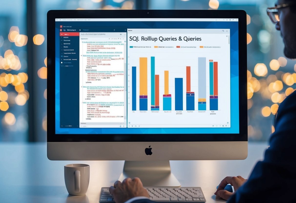
A computer screen displaying SQL rollup queries and data visualizations

The Group By clause in SQL can be enhanced using Rollup, which is used to create subtotals and grand totals. These functionalities help in making complex data analysis easier and more streamlined.

Grouping Sets and Rollup

A grouping set is a tool that enhances the Group By statement by allowing multiple groupings in a single query. It is especially helpful in SQL Server for simplifying aggregate calculations. The Rollup option expands the capabilities of grouping sets by automatically calculating subtotals along with the final grand total.

In MySQL, the Rollup modifier can be added to the Group By clause to enhance multi-level data analysis. By using Rollup, SQL queries can generate additional rows showing the subtotal of each grouping set, thus providing more detailed summaries of data.

Group By with Super-aggregate Rows

The Rollup function is a powerful extension of the SQL Group By clause. It not only helps in grouping data but also in creating super-aggregate rows, which include various dimensions and hierarchical levels. These rows represent subtotals of grouped data, and the final row is the grand total.

Using Rollup in SQL Server, users can streamline data analysis by combining different dimensions. The grand total row is particularly useful for overseeing overall data trends. When used correctly, it can greatly enhance the clarity and depth of data analysis within a single SQL query.

Implementing Rollup in SQL Databases
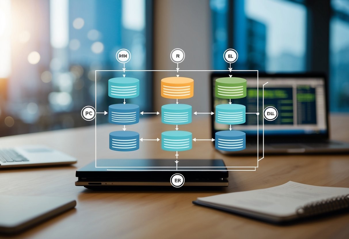
A database diagram with tables and columns, showing the implementation of SQL Rollups

SQL Rollup is an important tool for generating detailed reports by summarizing data. It extends the functionality of the GROUP BY clause, making it easier to calculate subtotals and grand totals in databases like Microsoft SQL Server and MySQL.

Rollup in Microsoft SQL Server

In Microsoft SQL Server, the Rollup is a subclause that simplifies generating multiple grouping sets. When an SQL query includes a Rollup, it creates summary rows, providing subtotals and a grand total row. This allows users to quickly analyze different levels of data aggregation within a single query.

For example, consider a sales table. By using Rollup, one can calculate total sales for each product category along with a cumulative total. This reduces the number of queries needed and increases efficiency.

Rollup is ideal for creating hierarchical reports that need different granularities of data.

Rollup in MySQL and Other Databases

In MySQL, Rollup is also used to generate aggregated results with subtotals and a grand total. Implementing Rollup in MySQL involves adding the Rollup operator to the GROUP BY clause in an SQL query, allowing the extension of summary data efficiently. This is especially useful for databases that require data to be grouped by different dimensions.

Rollup can provide insights by showing detailed data alongside summaries for evaluation. For other databases, the process might vary, but the core functionality remains consistent.

Ensuring that queries are well-structured can make data analysis more intuitive and informative.

Filtering Aggregated Data
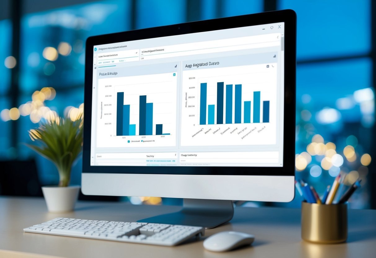
A computer screen displays a database query with aggregated data, while a chart visualizes SQL rollups

When working with SQL Rollups, filtering the aggregated data correctly is crucial. This process often involves using specific clauses to refine results and ensure meaningful data presentation.

Using Having with Rollup

The HAVING clause is a vital tool when filtering aggregated data in SQL, especially when using Rollup. Unlike the WHERE clause, which filters rows before aggregation, the HAVING clause applies conditions after data aggregation. This allows users to set conditions on the result of aggregate functions like SUM or COUNT.

For instance, when calculating total sales per product, HAVING can be used to show only those products with sales exceeding a specific threshold. This approach is useful in scenarios where users want to highlight significant data points without being affected by less relevant information.

Understanding the distinction and correct application of HAVING ensures precise data filtering after running rollup operations, which helps in generating cleaner and more readable reports.

Order By and Rollup

The ORDER BY clause enhances data presentation by arranging the output in a specified sequence. When combined with Rollup, it becomes even more powerful. This clause helps in sorting the final result set of aggregated data, allowing for easy comparison and analysis.

For example, after using Rollup to get sales totals per product, ORDER BY can sort these subtotals in either ascending or descending order. This clarity aids users in identifying patterns or trends within the dataset more quickly.

It is important to remember that logical sorting enhances the overall understanding of data, making it a key part of data analysis tasks.

Incorporating ORDER BY effectively ensures that the result set is not only complete but also arranged in a way that enhances interpretation and presentation.

Rollup in Business Intelligence Reporting

A stack of SQL textbooks surrounded by colorful charts and graphs

SQL rollups are essential in business intelligence for simplifying data and presenting clear insights. They’re used to create structured reports, analyzing sales trends, and streamlining inventory management by facilitating aggregate data analysis.

Constructing Sales Reports

In crafting sales reports, SQL rollups help summarize data by various dimensions, such as year, category, and region. This technique allows organizations to assess trends efficiently.

For example, a rollup can show sales by year, breaking down numbers into more detailed views, like sales by quarter or month, providing a clear timeline of performance. This enables businesses to evaluate seasonal trends and allocate resources effectively.

Additionally, analyzing sales by category can identify which products or brands are driving growth. It can highlight the success of specific marketing campaigns or the performance of various departments.

Rollups allow a detailed comparison of these dimensions, contributing to strategic decision-making by focusing on what’s most important.

Finally, using rollup in sales reports aids in constructing comprehensive dashboards that reflect key business insights, offering a bird’s-eye view while retaining the ability to drill down into specifics.

Rollup and Inventory Analysis

Rollup usage is significant in inventory management as well. It aggregates data across product lines, helping optimize stock levels. By summarizing data on stock counts by category or brand, managers can make informed decisions about restocking and discontinuation.

For example, understanding inventory levels across multiple locations can prevent stockouts and reduce excessive stock, saving costs.

Departments responsible for managing inventory can use rollups to analyze patterns, such as which items frequently run out or those with surplus stock. This is crucial for meeting demand without overstocking, which ties up capital.

Additionally, rollups can assist in forecasting future inventory requirements by analyzing past sales patterns and inventory turnover rates. They enable more precise predictions about which products need more attention in terms of supply chain and logistical planning.

Data Analysis with SQL Rollup

A computer screen displaying SQL code with rollup functions

SQL Rollup is an advanced feature that enhances data analysis by allowing efficient aggregation across multiple dimensions. It streamlines the reporting process and improves the ability to perform detailed data insights.

Multi-level Analyses

The rollup operator is integral for performing multi-level analyses in SQL queries. It functions by creating a series of subtotals that lead to a grand total, helping to break down complex data into more understandable parts.

For instance, in sales data, it can offer aggregated totals by product, month, and year. This technique saves time by eliminating the need for multiple queries for summary results, as seen in projects such as the SQL Pizza case study.

Using aggregate functions like SUM or AVG in ROLLUP operations helps generate different levels of aggregation. These functions allow users to gain valuable insights without extensive manual calculations.

The ROLLUP feature benefits businesses by offering summarized views that support informed decision-making.

Data Insight and Reporting Efficiency

The ROLLUP operator improves the reporting process by providing hierarchical grouping and easy-to-read insights. It efficiently handles large datasets by automatically grouping and summarizing data, which simplifies complex analyses.

For example, it can condense multiple sales metrics into summary tables, enhancing reporting efficiency.

By using the ROLLUP feature, businesses can not only save time but also improve accuracy. It removes the need for repetitive coding, making reports more efficient and insightful.

This structured approach allows analysts to focus on interpreting data trends rather than spending excessive time on data preparation.

Frequently Asked Questions

A stack of books on SQL with a magnifying glass and a pencil

The ROLLUP operation in SQL enables efficient data analysis by creating hierarchical summaries. It serves different purposes than the CUBE operation and is useful in situations where simple aggregation is needed over specific dimensions.

How does the ROLLUP operation function within GROUP BY in SQL?

The ROLLUP operation works as an extension of the GROUP BY clause in SQL. It allows for aggregated results to be calculated across multiple levels of a dimension hierarchy. By adding ROLLUP to GROUP BY, SQL creates subtotal and grand total summaries for the specified columns.

Can you provide an example of using ROLLUP in SQL?

Consider a sales database for an electronics store. Using ROLLUP, you can generate a report that includes sums of sales for each product category and a grand total.

For example, SELECT Category, SUM(Sales) FROM SalesData GROUP BY ROLLUP(Category) produces subtotals for each category and a single grand total row.

What is the difference between ROLLUP and CUBE operations in SQL?

While ROLLUP generates subtotal rows moving upwards in a hierarchy, CUBE provides a broader analysis. CUBE calculates all possible combinations of aggregations based on the given columns, effectively creating a multi-dimensional summary. This results in more detailed and varied grouping compared to ROLLUP.

What are the primary purposes of using a ROLLUP in SQL queries?

ROLLUP is primarily used for generating hierarchical data summaries. It helps in creating reports that include intermediate totals and a grand total, making it simpler to understand aggregated data.

This feature is essential for producing business reports and financial summaries where clarity and detail are necessary.

In what scenarios is it preferable to use ROLLUP over CUBE in SQL?

ROLLUP is preferable in scenarios where a straightforward hierarchy or a step-by-step summarization is needed. It is particularly useful when dealing with reports that require fewer aggregate calculations, such as sales by month followed by a yearly total, without needing all possible group combinations like CUBE.

How does the ROLLUP operation impact the result set in a SQL GROUP BY clause?

Using the ROLLUP operation, the result set from a GROUP BY clause includes additional rows for subtotal and total summaries. These rows contain aggregated data that are not available in a standard GROUP BY query.

This simplifies data analysis by providing clear insights at different levels of aggregation.

Categories
Uncategorized

Learning Pandas for Data Science – Time Series Essentials for Beginners

Getting Started with Pandas for Time Series Data

Pandas is a powerful Python library that simplifies data analysis, especially for time series data.

To get started, ensure pandas is installed. You can install it using the command:

pip install pandas

Once installed, pandas allows users to work with DataFrames, making it easier to manipulate and analyze data.

A common operation is reading data from a CSV file. This can be done using the read_csv function.

When working with time series data, it’s crucial to parse dates correctly. The read_csv function in pandas enables this by setting the parse_dates parameter.

For example:

import pandas as pd
df = pd.read_csv("data.csv", parse_dates=['date_column'])

This command reads a CSV file, ensuring the dates are parsed correctly, and stores the data in a DataFrame called df.

Time series analysis often involves manipulating DataFrames to focus on date-specific data. Pandas provides a variety of functions to filter and select data.

For instance, if you need to set the date column as an index:

df.set_index('date_column', inplace=True)

This step is essential for time-based operations like resampling or calculating rolling statistics.

Pandas also supports resampling of time series data to change the frequency of data points. This can be useful for summarizing data over specific intervals.

For example, monthly averages can be computed using:

monthly_avg = df.resample('M').mean()

This results in a new DataFrame with monthly averages.

Understanding Time Series Fundamentals

Time series analysis focuses on data points collected or recorded at consistent intervals. This forms the backbone for predicting trends and identifying patterns in various fields like finance, meteorology, and social sciences.

Recognizing specific elements within time series allows for precise analysis and forecasting.

Defining Time Series

A time series is a sequence of data points collected or recorded at specific times, usually at equal intervals. The key feature is its chronological order, which distinguishes it from other data types.

Common examples include daily stock prices or monthly sales figures. These data points are associated with a timestamp, often managed using a DatetimeIndex in programming libraries like pandas.

Time series data is used for observing and analyzing how variables change over time. This helps in predicting future trends and behaviors.

For example, economists might track the inflation rate over years to forecast future economic conditions.

Characteristics of Time Series Data

Time series data exhibits several important characteristics.

Trends reflect long-term increases or decreases in the data, like the steady rise in average global temperatures.

Seasonality indicates regular, repeating patterns or cycles, such as increased retail sales during the holiday season. Understanding these patterns is essential for accurate forecasting.

Data consistency, like having regular time intervals, is crucial for effective analysis. This is often handled using a date range to ensure all periods are represented.

Factors like missing data and irregular time-series can complicate analysis, requiring specific handling techniques to maintain data integrity. Recognizing these qualities helps in crafting effective models and predictions.

Data Structures for Time Series Analysis in Pandas

Pandas provides powerful tools for managing and analyzing time series data. The primary data structures used for this purpose are the Series and DataFrame, which support handling dates and times through DatetimeIndex and Time Stamps.

Series and DataFrame

A Series is a one-dimensional array-like structure in pandas. It can hold data of any type, and each element is associated with an index.

This structure is particularly useful for time series data, where each value has a specific date and time. The Series allows for easy slicing and dicing using indexes, making it simple to manipulate and analyze time-based data.

A DataFrame is a two-dimensional, table-like structure that can store data in rows and columns. It can be thought of as a collection of Series objects.

Each column in a DataFrame can have a different data type, and they are also indexed with labels. When working with time series data, DataFrames enable users to correlate data across different time series easily, perform aggregations, and visualize trends over time.

DatetimeIndex and Time Stamps

DatetimeIndex is a type of Index in pandas specifically designed for handling time-based data. It works with time stamps and is integral to time series analysis.

It supports various time operations such as shifting and resampling, which are crucial for aggregating and adjusting data frequencies.

Time Stamps are individual time-related data points. They are stored as datetime objects in pandas and allow users to work with a broad range of datetime functionalities, from simple operations like comparisons to more advanced ones like timezone conversion.

This makes time-based data analysis flexible and comprehensive, accommodating various formats and time zones.

Data Wrangling and Preparation for Time Series Modeling

Effective data preparation is essential for accurate time series modeling. This involves addressing missing data, transforming datasets, and aggregating information to enhance the analysis process.

Handling Missing Data

Dealing with missing values is crucial in time series data. Missing data can hinder analysis and model accuracy.

Techniques like forward fill and linear interpolation help manage gaps.

Forward fill copies the last known value to fill missing points and works well when trends are stable. Meanwhile, linear interpolation estimates missing values by calculating the line between two known points, which is useful for datasets with continuous trends.

Using the parse_dates parameter in Pandas can help smoothly handle date formats while loading data. It ensures dates are recognized and parsed correctly.

This is important for aligning and processing time-indexed data without errors. Accurate date parsing streamlines subsequent steps like aggregation and transformation, making the entire process more efficient.

Data Transformation and Aggregation

Data transformation is another key step. This process includes converting data into a format suitable for analysis.

Using methods like groupby or pivot in Pandas can restructure and summarize data.

Groupby allows for aggregation based on specific criteria, providing valuable summaries. For instance, calculating average values over monthly periods can reveal important trends.

Pivot tables enable transforming datasets to highlight relationships among variables. They can display data in a more accessible format, making patterns easier to spot.

Aggregation combines numerous data points into fewer, meaningful summary statistics, which simplify and improve the modeling stage.

Structured, organized data offers better insights and supports more precise predictive models.

Visualizing Time Series Data

Visualizing time series data is essential for uncovering trends and patterns that are not immediately apparent from raw data. It involves using Python libraries like Matplotlib and Seaborn to create informative and accurate representations.

Using Matplotlib and Seaborn

Matplotlib is a versatile library in Python, great for creating detailed and complex plots. It allows users to control every element of a graph, making it ideal for time series analysis.

For instance, users can plot dates on one axis and data points on another, easily seeing changes over time.

Seaborn builds on Matplotlib’s features by providing a high-level interface for drawing attractive and informative statistical graphics. It includes built-in themes and color palettes that improve the aesthetics of plots.

It simplifies the creation of complex visualizations, making it easier for data scientists to understand and explain time-dependent behaviors.

Plotting Trends and Seasonality

Identifying trends in time series data is crucial for predicting future values. Simple line plots can show upward or downward trends over time, which are essential for forecasting.

These trends can be overlaid with moving averages to smooth out short-term fluctuations.

Seasonality refers to patterns that repeat at regular intervals. Visualizing seasonality involves plotting data over multiple time periods, such as months or quarters.

Techniques like heat maps can be used to display data across a calendar format, making it easier to spot recurring seasonal patterns.

Recognizing these patterns helps in making informed decisions based on recurring events or cycles in the data.

Statistical Analysis of Time Series

Time series analysis often involves understanding patterns and characteristics in data, such as identifying dependencies between observations. Autocorrelation measures how observations in a series relate to each other. Differencing is a method to make non-stationary data stationary, crucial for effective modeling.

Autocorrelation and Partial Autocorrelation

Autocorrelation indicates how current values in a time series are related to past values. It is measured using the autocorrelation function (ACF), which shows correlations at different lags.

High autocorrelation at a specific lag means past values influence current values.

Partial autocorrelation (PACF) helps isolate the direct relationship between current and past values without interference from intermediate lags.

PACF is useful in identifying the order of autoregressive models, by showing only the correlation of a lag once the relationships of shorter lags have been accounted for.

Recognizing patterns in autocorrelation and partial autocorrelation is crucial for building effective statistical models.

Stationarity and Differencing

A stationary time series has constant mean, variance, and autocovariance over time. Many statistical models assume stationarity, making it vital to assess and ensure data meets this criteria.

Non-stationary data often exhibit trends or seasonal patterns, complicating the analysis.

Differencing is a common technique used to transform non-stationary data into stationary data. By calculating the differences between consecutive observations, differencing removes trends and stabilizes variance.

This process aids in simplifying the analysis and improving model accuracy when predicting future values.

Recognizing whether data is stationary or non-stationary informs the choice of model and preprocessing steps, ensuring reliable results.

Essential Time Series Forecasting Methods

Time series forecasting involves predicting future values based on previously observed data points. This section explores several key forecasting methods used widely in data science to manage and interpret time series data effectively.

Moving Averages

Moving averages smooth out short-term fluctuations and highlight longer-term trends in data. This technique is often used with rolling windows, where the average is computed over a specific number of past observations.

There are different types of moving averages, including simple and weighted.

The simple moving average (SMA) gives equal weight to all observations, while the weighted moving average assigns more importance to recent data points. This can help in identifying the current trend more accurately.

Moving averages are foundational for more complex forecasting methods and are easy to implement with libraries like Pandas.

Exponential Smoothing

Exponential smoothing forecasts are made by applying smoothing factors to past observations. Unlike moving averages, this method gives exponentially decreasing weights to older observations.

This approach includes several methods like Simple Exponential Smoothing (SES) for data without trend or seasonality and Holt’s Linear Trend Model, which accommodates data with trends.

Holt-Winters Seasonal Model, a more advanced method, accounts for both trend and seasonality.

These techniques allow for flexible adjustment to match data characteristics and are critical in applications where recognition of patterns quickly is important, such as stock market analysis or inventory management.

ARIMA and Seasonal ARIMA

ARIMA, which stands for AutoRegressive Integrated Moving Average, is a more sophisticated method combining regression of past values, differencing to ensure stationarity, and a moving average model.

It’s essential for data that exhibit complex patterns not handled by basic models.

Seasonal ARIMA (SARIMA) extends this by incorporating seasonal differences, making it highly effective for data with regular seasonal patterns.

Proper configuration of ARIMA and SARIMA models requires selecting the right parameters, which involves testing and optimizing using techniques like the Akaike Information Criterion (AIC) for the best forecast results.

These models are widely used in various domains, from economics to weather forecasting.

Machine Learning for Time Series Prediction

Machine learning techniques are essential for making sense of time series data.

Key approaches include linear regression models, tree-based models like random forests, and deep learning techniques. Each method has unique benefits and applications, providing powerful tools for accurate forecasts.

Linear Models for Regression

Linear regression models serve as a fundamental method for time series prediction. They establish relationships between dependent and independent variables using a linear equation. Despite their simplicity, these models are effective for certain types of time series data.

With the use of libraries like scikit-learn, fitting linear models becomes straightforward. The models are interpretable, making them useful for data with linear trends.

It’s crucial to preprocess data to deal with issues like autocorrelation and seasonality before applying linear regression.

Tree-Based Models

Tree-based models, such as random forests, provide a robust alternative to linear models. They work by creating a series of decision trees, each contributing to the final prediction. These models can capture complex patterns in time series data, making them versatile.

Random forests, in particular, handle non-linear relationships and interactions between variables effectively. This makes them ideal for datasets where traditional linear models struggle.

Using a test set to evaluate their performance ensures reliable and unbiased results.

Deep Learning Approaches

Deep learning offers advanced methods for predicting time series data. Techniques such as Recurrent Neural Networks (RNNs) and Long Short-Term Memory (LSTM) networks excel in capturing sequential dependencies and non-linear patterns.

These approaches are particularly useful for large datasets where patterns are intricate and high-dimensionality exists.

They require more computational power but benefit from their ability to learn complex representations.

While deep learning models can be powerful, tuning their many parameters requires expertise and careful validation against a test set for accurate forecasting.

Advanced Time Series Models

A laptop displaying a time series data analysis using Pandas, with various charts and graphs on the screen

Exploring advanced time series models can enhance the accuracy of predictions in data science.

This section covers two popular methods that include statistical and machine learning models to handle complex datasets with seasonal patterns and other factors.

SARIMAX and Prophet

SARIMAX (Seasonal AutoRegressive Integrated Moving Average with eXogenous factors) is an extension of the ARIMA model. This model handles data with trends and seasonality, making it suitable for datasets with complex patterns.

SARIMAX allows for external variables, which can improve the model’s ability to predict future values accurately. It requires careful tuning of parameters like p, d, and q, alongside seasonal counterparts P, D, and Q.

Prophet, developed by Facebook, is designed for time series with daily observations of multiple seasonalities. It is highly customizable and suitable for handling missing data well, making it effective for business forecasts.

Unlike SARIMAX, Prophet requires minimal input for tuning due to its automatic adjustment capabilities, providing an intuitive way to work with time series data.

BATS and TBATS Models

BATS (Box-Cox transformation, ARMA errors, Trend, and Seasonal components) is engineered to fit time series with complex seasonal effects. This model includes Box-Cox transformation for data stabilization, ARMA errors to manage residuals, and components to model trends and seasons. BATS is versatile in handling series with multiple seasonal periods.

TBATS (Trigonometric BATS) extends BATS by incorporating trigonometric terms, improving seasonality representation in time series data. TBATS is particularly beneficial when dealing with time series with high-frequency seasonal patterns.

These models are flexible and allow for handling irregular observed frequencies and varying season lengths, key aspects in advanced time series analysis.

Analyzing Real-World Time Series Datasets

Time series data is invaluable for understanding patterns and trends over time. Real-world datasets in electricity consumption and renewable energy production are prime examples for performing exploratory data analysis (EDA) and gaining insights into operational dynamics.

Electricity Consumption

Electricity consumption datasets offer rich insights into usage patterns. These datasets often consist of historical data, showcasing variations in demand across different times of the day, week, and year.

Analyzing this data helps identify peak usage periods and potential savings opportunities.

With exploratory analysis, patterns such as seasonal fluctuations and daily usage cycles can be uncovered. Visual tools like line charts and heatmaps are effective for spotting trends and anomalies.

Recognizing these patterns supports better forecasting and management strategies in energy distribution.
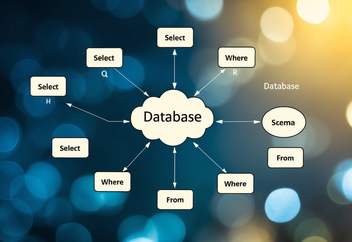
Wind and Solar Power Production

Wind and solar power production datasets provide valuable information on energy generation patterns. These datasets often include real-world data collected over long periods, capturing variations due to weather conditions and geographical factors.

Thorough analysis reveals how environmental factors influence production levels and identify periods of peak generation.

For exploratory analysis, integrating meteorological data can be insightful. Data analysts use EDA techniques to visualize correlations between weather patterns and energy output.

Understanding these relationships helps optimize energy planning and integration of renewable sources into the grid.

Appropriately using this data supports sustainable energy solutions and efficient resource management.

Performance Metrics and Model Evaluation

A computer screen displaying time series data with various performance metrics and model evaluation charts

Evaluating model performance in data science is crucial, especially for time series and forecasting tasks. Understanding the metrics used for evaluation helps in choosing the best model.

Forecasting Methods: When predicting future data points, it’s important to select the right metrics.

Common metrics include Mean Absolute Error (MAE) and Root Mean Square Error (RMSE). These help in assessing how well a model forecasts future values.

Regression Metrics: In regression tasks, metrics such as R-squared and Mean Squared Error (MSE) are widely used. These metrics measure the accuracy of model predictions compared to actual data.

Test Set Usage: A test set is essential for evaluating the model’s performance on unseen data. It ensures that the model’s predictions are not just accurate on training data.

Time Series Analysis: In this context, metrics like autocorrelation and stationarity tests are used. These help in understanding data patterns and ensuring that time series models are robust.

The use of both statistical models and machine learning techniques can enhance model accuracy.

Machine learning models, such as those using deep learning, often require careful evaluation to prevent overfitting.

Practical Tips for Time Series Projects

When handling time series data, understanding the unique traits of sequential data is crucial. Time series often require specific methods for cleaning and preprocessing, such as handling missing values and resampling data for uniform intervals.

Data visualization is key in time series analysis. It helps to spot trends, seasonality, and anomalies.

Use plots like line graphs and heatmaps to represent data over time clearly.

For successful data science projects involving time series, using libraries like Pandas is beneficial. They offer tools for easy manipulation and analysis.

For example, Pandas provides functions to read and process time-oriented data efficiently.

Project management plays a vital role. Define clear goals and objectives at the beginning. This helps in aligning the analysis with business needs and expectations.

Consider these best practices:

  • Data Quality: Ensure your data is clean and consistent. Check for missing or out-of-range values regularly.
  • Scaling and Transformation: Often, time series data must be normalized or transformed.
  • Validation: Use cross-validation to test models. Splitting data into training and testing sets helps in assessing the model’s performance.
  • Collaborative Tools: Utilize tools for sharing code and insights. GitHub and similar platforms are helpful for collaborative projects.

By adopting these strategies, data analysts can navigate time series projects more effectively, accommodating both technical aspects and project management needs.

Frequently Asked Questions

Pandas is a powerful library for handling time series data. It is essential for converting DataFrames, plotting by groups, creating date ranges, and managing timestamps. The way Pandas supports various data types makes it versatile for time-related tasks.

How do I convert a DataFrame into a time series in Pandas?

To convert a DataFrame into a time series, set the date column as the index using set_index(). This allows you to leverage time-based indexing features.

Use pd.to_datetime() to ensure the date column is in the correct format.

What are the best practices for time series analysis in Pandas?

Ensure your data is clean and in the correct datetime format. Use resampling to match the time frequency required for analysis.

Handling missing data with methods like forward or backward fill is beneficial for maintaining consistency.

How can I use Pandas to plot a time series by groups?

Group data using the groupby() function and then plot using the plot() method. This approach helps visualize trends across different segments.

Utilize matplotlib for additional customization of the plots.

Which function in Pandas should I use to create a date range for time series data?

Use pd.date_range() to create a date range. This function is crucial for generating sequences of dates with specified frequency.

It helps in forming a complete time series that suits your needs.

Can you explain how to handle timestamps and time-related features using Pandas?

Pandas provides Timestamp objects to handle single time stamps, and Timedelta for duration.

Use dt accessor to retrieve time features like year, month, day, etc. This can automate and simplify time-based operations.

What data types does Pandas support for time series data?

Pandas primarily uses datetime64 for dates. It also supports Period and Timedelta for more specific time representations. These types ensure precise handling of different time series requirements.

Categories
Uncategorized

Learning Math for Machine Learning – Probability Fundamentals Explained

Probability Foundations

Probability foundations are crucial for understanding how algorithms make decisions under uncertainty. This section introduces the fundamentals of probability theory and explains the basics of combinatorics, which is essential for counting possibilities in various scenarios.

Probability Theory Basics

Probability is the study of how likely events are to occur. In mathematics, it is represented as a number between 0 and 1. An event with a probability of 1 is certain to happen, while an event with a probability of 0 is impossible.

Key concepts in probability theory include random variables, which are variables whose outcomes are determined by chance, and probability distributions, which describe how probabilities are distributed over the possible outcomes.

Understanding conditional probability is also important. It is the probability of an event occurring given that another event has already happened.

Bayesian probability is another approach, relying on prior knowledge to update the probability estimates as more data becomes available. This probabilistic approach is often used in machine learning for developing predictive algorithms.

Combinatorics and Counting

Combinatorics is an area of mathematics focused on counting, arranging, and combining items. It plays a key role in probability, especially in determining the number of ways an event can occur.

Basic concepts in combinatorics include permutations and combinations. Permutations are arrangements where the order matters, while combinations are selections where order does not matter.

For instance, in algorithms, combinatorics can help decide the number of possible states or configurations in a problem. This branch of mathematics enables precise calculation in probability theory, making it a vital tool for machine learning.

Understanding Variables and Distributions

Understanding variables and probability distributions is key in machine learning. Variables can change and be described using different distributions, like normal or binomial. Knowing these concepts helps in analyzing data accurately.

Random Variables

Random variables are crucial in statistics and machine learning. They represent potential outcomes of experiments. For example, in rolling a die, a random variable can denote the number on the top face.

There are two main types: discrete and continuous. Discrete variables have specific values, like counting students in a class. Continuous variables can take any value within a range, such as measuring a person’s height. Understanding these distinctions helps in selecting the right tools and methods for analysis.

Random variables are often represented as vectors. These can contain multiple values, each corresponding to different outcomes. This approach helps in analyzing experiments with numerous possibilities.

Common Probability Distributions

Probability distributions describe how outcomes of a random variable are spread out. Some common types include normal, binomial, and Poisson distributions. Each has its unique properties and applications.

The normal distribution is symmetric and bell-shaped, often used in natural and social sciences. It is defined by its mean and variance. A key feature is its mode, which is the peak of the distribution curve.

The binomial distribution is used for experiments with two possible results, like flipping a coin. It is defined by the number of trials and probability of success in each trial.

The Poisson distribution models the number of events in a fixed interval of time or space, such as the number of emails received in an hour. Understanding how these distributions work aids in choosing the right model for data analysis.

Mathematics for Machine Learning

A chalkboard filled with mathematical equations and diagrams related to probability, surrounded by books and computer screens

Understanding mathematics is essential for building and refining machine learning models. Two key areas are calculus and linear algebra, which help explain how algorithms optimize and manage complex data structures.

Calculus Review

Calculus is used to optimize algorithms, enhancing the efficiency of machine learning models. Concepts like differentiation and integration help in understanding how changes in input variables affect outcomes.

Derivatives are used to minimize or maximize functions, crucial for tasks like minimizing error in predictions. Meanwhile, gradient descent, a popular optimization method, relies heavily on calculus to iteratively adjust weights and biases in neural networks.

By understanding calculus, developers can fine-tune models to achieve greater accuracy and performance.

Linear Algebra Essentials

Linear algebra forms the backbone of machine learning calculations. It deals with vectors, matrices, and linear transformations.

Machine learning algorithms often require manipulation of large data sets and matrices, making linear algebra an indispensable tool.

Operations like matrix multiplication help in expressing complex operations in a compact form which is useful in various aspects, from data preprocessing to the implementation of neural networks.

Engineers use concepts such as eigenvectors and eigenvalues for dimensionality reduction, crucial in managing high-dimensional data spaces. Understanding linear algebra is vital for anyone looking to excel in the field of machine learning.

Statistical Principles in Data Science

Statistical principles play a critical role in data science by allowing practitioners to summarize, analyze, and draw conclusions from data. They require strong math skills to understand and apply various statistical methods effectively.

Descriptive Statistics

Descriptive statistics provide simple summaries about the sample and the measures. They form the basis of virtually every quantitative analysis of data.

Measures such as mean, median, and mode describe the central tendency, while range, variance, and standard deviation explain data variability.

Tables and charts are often used to represent these measures visually.

Descriptive statistics are crucial in exploratory data analysis, helping data scientists see patterns or trends before diving into more complex analyses. By summarizing data sets, they offer a helpful overview, making large amounts of data digestible. This approach simplifies data interpretation and determines the initial insights needed to explore cause-and-effect relationships further.

Inferential Statistics

Inferential statistics go beyond mere summaries and deal with making predictions or inferences about a population based on a sample.

Using tools like hypothesis testing, confidence intervals, and regression analysis, data scientists can infer trends and patterns and make data-driven decisions.

These methods rely heavily on the principles of probability to quantify the degree of uncertainty involved in drawing conclusions from the data.

Inferential statistics are essential when working with large data sets where full data analysis is impractical. They support the testing of hypotheses to validate assumptions, enabling evidence-based decision-making that is integral to many applications in data science.

Exploration of Algorithms and Structures

A stack of math textbooks surrounded by geometric shapes and computer code, with a focus on probability theory and machine learning algorithms

Understanding algorithms and data structures is essential in computer science and engineering. They form the backbone of machine learning models and influence their efficiency and accuracy. This section discusses the foundational principles of algorithms and the importance of selecting appropriate data structures.

Algorithmic Foundations

Algorithms are step-by-step procedures or formulas for solving problems. They play a critical role in computer science by optimizing processes and making complex tasks manageable.

In machine learning, algorithms are used to train models, allowing computers to learn from data and make predictions.

Key elements of algorithms include correctness, efficiency, and scalability.

Ensuring an algorithm runs correctly and efficiently is paramount for optimal performance. Engineers and computer scientists develop different types of algorithms, such as searching and sorting algorithms, to enhance processing speed.

Understanding these core areas helps in creating more sophisticated and intelligent models that can process large datasets effectively.

Data Structures and Their Importance

Data structures organize and store data efficiently, enabling quick access and modification.

Choosing the right data structure can significantly affect the performance of machine learning algorithms.

Common structures include arrays, linked lists, stacks, and queues, each with unique benefits.

For example, arrays provide fast access to elements, while linked lists offer efficient memory use. The use of advanced structures like trees and graphs can optimize complex operations.

In engineering, understanding how to implement and manipulate these structures aids in solving real-world problems.

Selecting appropriate structures is crucial for enhancing the scalability and efficiency of machine learning systems, ultimately improving their ability to handle large volumes of data successfully.

Programming for Mathematical Computing

A computer displaying code for mathematical computing with a focus on probability, surrounded by books on machine learning and math

Programming is essential in mathematical computing, serving as the backbone of implementing algorithms efficiently. Notably, Python plays a crucial role, offering versatility and a range of libraries. Writing efficient code for mathematical operations is key to optimizing performance in machine learning tasks.

Python in Machine Learning

Python is a highly favored language for machine learning due to its simplicity and robust libraries like NumPy, SciPy, and TensorFlow.

These tools allow developers to handle complex mathematical computations seamlessly.

NumPy provides support for large multi-dimensional arrays and matrices, along with a collection of mathematical functions to operate on these arrays.

SciPy extends this functionality to provide further modules for optimization and signal processing.

For those working on machine learning models, the ability to process large datasets efficiently is essential.

Libraries like TensorFlow and PyTorch are widely used for building and training machine learning models, enabling the execution of tasks across various platforms.

These libraries support both CPU and GPU, making them versatile for different computing needs.

Efficient Code for Mathematical Operations

Writing efficient code involves optimizing algorithms to reduce computational time and resource usage. This is particularly significant when working with large datasets or complex calculations.

Techniques such as vectorization, which is supported by NumPy, help in speeding up the execution by performing batch operations on data.

Utilizing built-in functions and avoiding loops where possible can drastically decrease execution time.

Python’s extensive library support provides optimized algorithms for common tasks. For instance, using libraries like SciPy for linear algebra operations ensures that the most efficient algorithms are employed, often leveraging underlying compiled code for speed.

Parallel computing is another strategy, utilizing libraries like Dask to distribute work across multiple cores or nodes.

This allows for the handling of massive datasets and intensive computation, making programming for mathematical computing both efficient and scalable.

Machine Learning Model Fundamentals

A computer displaying probability equations and graphs for machine learning

In machine learning, understanding the types of learning models is crucial. Supervised learning involves training models with labeled data, while unsupervised learning uses data without explicit labels. Both methods have distinct approaches and applications.

Supervised Learning

Supervised learning uses labeled datasets to train models in predicting outcomes.

Common methods include linear regression, which predicts continuous values, and classification techniques for categorizing data. For instance, email spam detection falls under this category.

Neural networks can enhance supervised learning by enabling complex pattern recognition in data.

These models typically require a large amount of accurately labeled data and are evaluated using metrics like accuracy and precision.

Challenges in supervised learning include overfitting, where a model learns noise rather than meaningful patterns. To counter this, techniques like cross-validation and regularization are employed. These methods ensure models perform well on new, unseen data.

Unsupervised Learning

Unsupervised learning works with data that lacks explicit labels, allowing models to find hidden patterns or groupings.

Techniques like clustering and dimensionality reduction are common. Clustering groups data based on similarities, useful in customer segmentation, while dimensionality reduction simplifies data, which can enhance performance in higher-dimensional datasets.

Neural networks in unsupervised learning, such as autoencoders, assist in feature learning and generation of new data formats.

Unlike supervised methods, unsupervised learning does not provide specific predictions but identifies data structures that weren’t obvious. These insights are essential for data exploration and preliminary analysis, aiding the development of further machine learning models.

Data Handling and Manipulation

A computer screen displaying a graph with data points, a calculator, and a textbook open to a page on probability

Data handling and manipulation are vital when working with machine learning models. These processes include organizing and preparing data for analysis. Methods in linear algebra, like matrix operations, play a key role in this, transforming data for better machine learning performance.

Working with Matrices

Matrices are essential in machine learning for structuring data.

Matrix multiplication is a common operation that facilitates various machine learning tasks.

When data is in matrix form, it allows for efficient calculations, such as transforming datasets using transformations.

In linear algebra, understanding the structure of matrices can help in dimensionality reduction. This is crucial for simplifying datasets without losing important information.

Singular value decomposition (SVD) is a technique used for this purpose, helping models perform better by reducing computational load.

Matrices also support operations like inversion and transposition, which are important in algorithms like regression analysis.

By leveraging matrices, complex data relationships become easier to interpret, enhancing the effectiveness of machine learning models.

Data Preprocessing Techniques

Preprocessing prepares raw data, improving the quality of input data for machine learning.

This involves cleaning, transforming, and encoding data to make it suitable for analysis.

Techniques include scaling, where features are adjusted to fit within a certain range, making models more robust.

Handling missing values is another important step. Methods like imputation fill in gaps where data is incomplete, ensuring that models do not encounter errors during training.

Encoding categorical data transforms categorical values into numerical formats, enabling algorithms to process them effectively.

Other preprocessing methods involve filtering noise from data.

Techniques such as normalization and standardization ensure that different variables contribute equally to the analysis, promoting better model performance and accuracy when predicting outcomes.

Dimensionality and Its Challenges

A complex web of interconnected nodes and lines representing mathematical probability concepts

Dealing with high-dimensional data is a core challenge in machine learning. It involves handling numerous variables or features, which can complicate analysis and increase the risk of overfitting models.

Solutions like dimensionality reduction are key in streamlining the process and improving outcomes.

Understanding Dimensionality

Dimensionality in machine learning refers to the number of features or variables used to describe data. As the number grows, the complexity of the problem can increase.

This phenomenon, often called the “curse of dimensionality,” can make it hard to model data accurately.

In high dimensions, data points can appear sparse. This sparseness can affect algorithms, making them less reliable due to a lack of nearby data points for accurate predictions.

Moreover, calculations involving distances, such as clustering and nearest neighbor algorithms, can become less effective.

Dimensionality also impacts storage and computation. High-dimensional data can require significant computational resources.

It is vital to balance the benefits of additional features with the costs related to processing and storage.

Approaches to Dimensionality Reduction

Dimensionality reduction techniques help mitigate the challenges of handling high-dimensional data. These methods aim to reduce the number of input variables while retaining as much information as possible.

Common techniques include Principal Component Analysis (PCA) and t-Distributed Stochastic Neighbor Embedding (t-SNE).

PCA is widely used and works by transforming data into a new set of variables called principal components. These components capture the most variance in the data.

t-SNE is particularly useful for visualizing high-dimensional data by mapping it to lower dimensions.

Feature engineering also plays a role in dimensionality reduction.

It involves creating new features from existing ones, which can better represent the underlying patterns in the data.

By doing this, engineers can often reduce the dimensions without losing critical information, making models more efficient and effective.

Learning Resources and Pedagogy

A chalkboard filled with mathematical equations, graphs, and probability diagrams, surrounded by colorful math manipulatives and educational resources

Exploring effective ways to learn probability for machine learning involves both innovative teaching methods and various resources for self-learners.

Innovative Teaching Methods

Educators are continually developing new strategies to improve how students learn probability.

One approach is using modeling in teaching, which helps students visualize complex problems by creating real-world scenarios. These models make abstract concepts more tangible.

Another effective method is integrating games into the curriculum, which studies have shown can boost engagement and understanding.

Research suggests that games create interactive and participatory learning environments. This engagement helps students develop practical skills necessary for understanding probability.

A blend of traditional and modern pedagogical tools can cater to different learning styles, ensuring a comprehensive learning journey for students.

Resources for Self-Learners

For those who prefer self-directed learning, a variety of resources are available.

Digital platforms, such as e-learning courses, provide access to high-quality content. These platforms often include videos, quizzes, and practical exercises, helping learners grasp difficult concepts at their own pace.

Textbooks remain a valuable resource, offering structured content and exercises for in-depth study.

Some textbooks focus on promoting a deep understanding of mathematical principles, guiding learners with step-by-step approaches.

Furthermore, educational websites and forums offer additional support, allowing self-learners to collaborate and engage with a community of peers.

These resources empower learners to explore probability in a flexible and comprehensive manner.

Real-World Applications of Probability

Probability plays a vital role in transforming theoretical concepts into practical applications across various fields. It is crucial for making predictions and decisions in technology and engineering.

Applications in Artificial Intelligence

Probability is fundamental in the field of artificial intelligence, especially in machine learning.

It helps in developing models that can predict outcomes and make decisions based on data. Techniques like logistic regression use probabilistic methods to assess data and determine probabilities.

In AI, probabilistic models are used to handle uncertainties and make decisions under uncertain conditions.

Bayesian networks, for example, model relationships between different variables and update their beliefs as more data becomes available. This is key for applications like speech recognition, where the system must decide between multiple possible interpretations.

Probabilistic Models in Engineering

Engineering uses probabilistic models to improve design and decision-making processes. These models help predict failure rates and optimize systems for reliability.

In civil engineering, for instance, probability is used to analyze and mitigate risks such as structural failure.

By applying probabilistic concepts, engineers can anticipate potential issues and design safer structures.

In electronics, probabilistic methods are utilized to evaluate circuit performance under varying conditions.

These approaches ensure components work effectively under uncertain and dynamic environments. Thus, probability is not only an analytical tool but also a crucial aspect of innovative design and safety assurance in engineering projects.

Career Paths and Progression in Data Science

A computer screen displaying a graph of probability distribution with mathematical equations and data science career progression paths in the background

Data science offers various career paths, including roles in data analysis, engineering, and research. Each path requires specific skills and experiences. Learning doesn’t stop after becoming a data scientist. Continuous education and specialization can lead to advanced positions.

Becoming a Data Scientist

To become a data scientist, one generally needs a strong foundation in mathematics, statistics, and computer science.

Key skills include:

  • Programming languages: Python and R
  • Statistics and probability
  • Machine learning algorithms

Gaining experience through internships or projects can be very helpful. Entry-level roles often include data analyst or junior data scientist positions.

Certifications in data science can also boost a candidate’s resume and increase job prospects. Networking and joining professional organizations like the Data Science Society can help in finding opportunities and advancing one’s career.

Further Studies and Specializations

In data science, continuous learning is important.

Professionals may choose to specialize in areas like:

  • Machine learning engineering
  • Data mining techniques
  • Artificial Intelligence (AI)

Pursuing a Master’s or PhD in data science or related fields can open doors to research positions or advanced roles such as senior data scientist or data science manager.

Specialized certifications in tools like TensorFlow or Hadoop can also enhance one’s skills and job appeal. Engaging in workshops and conferences helps stay updated with industry trends and technologies.

Frequently Asked Questions

Understanding probability is crucial for developing effective machine learning algorithms. This section looks at the essential concepts, the role of probability in enhancing model performance, and key resources for learning.

What are the fundamental probability concepts necessary for understanding machine learning algorithms?

Key concepts include random variables, probability distributions, expectation, variance, and independence. These form the backbone of statistical models, helping to interpret data and predict outcomes.

How does a solid grasp of probability and statistics enhance model accuracy in machine learning?

A strong foundation in probability allows the machine learning practitioner to effectively handle uncertainty and variability in data. This knowledge leads to better algorithm tuning, improved data sampling techniques, and more accurate predictions.

Which probability distributions are most commonly used in machine learning and why?

Common distributions include the normal, binomial, and Poisson distributions. These are frequently used because they model a wide range of phenomena and support various machine learning tasks, such as classification and regression.

In what ways is Bayes’ theorem applicable to machine learning models?

Bayes’ theorem is used in updating the probabilities of hypotheses as more evidence becomes available. It plays a critical role in classification problems and in models like the Naive Bayes classifier.

Can you recommend any comprehensive resources for learning about probability in the context of machine learning?

“Python for Probability, Statistics, and Machine Learning” offers extensive code examples and is available on Springer. Additionally, “Probabilistic Machine Learning: An Introduction” provides insights into probabilistic frameworks and can be accessed through Google Books.

Why is an understanding of probability essential for evaluating the performance of a machine learning model?

Probability is vital for evaluating model performance. It helps in understanding model behavior, assessing uncertainty in predictions, and making data-driven decisions. This leads to more reliable and robust performance evaluations.

Categories
Uncategorized

Azure Data Studio Extensions: Enhance Your Database Experience

Understanding Azure Data Studio

Azure Data Studio is a versatile tool developed by Microsoft for data management and development. It supports platforms such as Windows, macOS, and Linux. This makes it accessible to a wide range of users who work with databases in different environments.

One of the standout features of Azure Data Studio is its interface, which is reminiscent of Visual Studio Code. This familiarity is helpful to developers who have used Visual Studio Code, making the transition to Azure Data Studio smoother.

Cross-platform support is an essential feature. Azure Data Studio can connect seamlessly to popular cloud databases like Azure SQL and SQL Server.

Users can also connect to other databases, such as MySQL, PostgreSQL, and MongoDB, by adding extensions.

Additionally, Azure Data Studio is designed with cloud and on-premises databases in mind, so it’s suitable for various database management tasks. Its flexibility allows developers to query, design, and manage their databases effectively.

Extensions play a significant role in expanding the functionality of Azure Data Studio. They are available from both Microsoft and the community, offering a range of tools and functionalities to enhance the user experience.

For those looking to customize their experience, Azure Data Studio’s extension library offers many options. The ability to add new features as needed helps tailor the tool to individual needs, making it an indispensable resource for developers and data professionals.

Core Extensions for Enhanced Functionality

Azure Data Studio offers several essential extensions that enhance its capabilities, especially for SQL Server management and administration. These extensions help professionals efficiently handle various tasks, using familiar tools found in SQL Server Management Studio (SSMS).

SQL Server Agent

The SQL Server Agent extension is crucial for managing automated tasks. It allows users to schedule and execute routine jobs without manual intervention. This tool is particularly valuable for database administrators who need to manage repetitive T-SQL scripts or maintenance plans.

With this extension, users can create, edit, and manage SQL Server jobs directly from Azure Data Studio. It includes features like job history and alerts to monitor and troubleshoot any issues.

SQL Server Profiler

SQL Server Profiler is an extension that allows users to capture and analyze database events. It is useful for diagnosing slow queries, detecting problematic T-SQL code, and ensuring SQL Server performance optimization.

This tool mirrors the capability found in SSMS, helping users monitor live queries and identify long-running ones. Profiling in Azure Data Studio allows users to filter and sort events for targeted analysis, all integrated into one platform.

SQL Server Import

The SQL Server Import extension simplifies data import tasks. It is designed for users who need to quickly import spreadsheets or flat files into SQL Server databases. This tool supports various file formats, making data migration a straightforward process.

Using this extension, users can map source data to target SQL Server tables with an intuitive interface, allowing for seamless integration. Importing data has never been easier, reducing the need for complex scripting.

SQL Server Database Administration

Database administrators can leverage the SQL Server Database Administration extension for comprehensive management features. This extension offers insights into performance metrics, backup processes, and database integrity. It also supports managing DACPAC files for deploying and versioning databases.

Through the Extensions Manager, users can install and configure this extension to monitor server health, perform routine database checks, and optimize storage usage. It integrates tasks performed in SSMS, ensuring Azure Data Studio remains a robust tool for database administrators.

Database Development Workflows

The use of Azure Data Studio extensions enhances database development by managing SQL databases, tracking query history, and working efficiently with stored procedures and tables. These tools allow for streamlined workflows within the development environment.

Query History

Azure Data Studio keeps a detailed history of queries, which helps developers track past activities. This feature saves time by allowing them to revisit and rerun past queries. Users can filter through this history by workspace or timeline to quickly find important queries.

This capability is particularly useful in troubleshooting. By examining previous queries, it is easier to pinpoint errors or optimize performance. The integration with source control also means developers can maintain a consistent workflow.

SQL Databases Management

Managing SQL databases efficiently is vital for robust database development. Azure Data Studio supports connectivity to various databases such as Azure SQL, SQL Server, MySQL, and PostgreSQL. Users can easily connect to these from within the development interface.

The extension library expands this capability, allowing developers to work with different database types. This versatility aids in designing, editing, and publishing database schemas.

With features like schema comparison and automated deployment via CI/CD pipelines, managing SQL databases becomes highly efficient.

Stored Procedures & Tables

Stored procedures and tables are essential in organizing and executing SQL commands. Azure Data Studio provides tools to create and edit these components seamlessly.

Developers can use the SQL Database Projects extension to build source-controlled projects, ensuring consistency across development and production environments.

The extension supports designing complex stored procedures with version control. Tables and their relationships can be visualized, aiding in better understanding and efficient database management.

These capabilities simplify the development process, allowing developers to focus more on optimizing their databases. With these tools, both novice and experienced users can manage stored procedures and tables effectively.

Performance and Administration Tools

A desk with a computer monitor displaying azure data studio extensions. Various tools and administrative features are visible on the screen

In Azure Data Studio, performance and administration tools are essential for database administrators and developers managing different databases. These tools help in monitoring, analyzing, and optimizing database performance. They offer features to simplify tasks and increase efficiency across platforms like SQL Server, PostgreSQL, and Azure SQL Database.

Server Reports

Server reports provide a visual overview of server performance, helping administrators make informed decisions. These reports can show key metrics like CPU usage, memory consumption, and query performance.

By utilizing these reports, users can quickly identify bottlenecks or resource-intensive queries. This insight is crucial for maintaining optimal performance levels and ensuring that resources are used efficiently. Extensions in Azure Data Studio offer access to these reports, making them accessible and easy to use. Regularly reviewing server reports can also aid in predicting future needs and addressing potential issues before they escalate.

Whoisactive

Whoisactive is a powerful tool for identifying active sessions and queries running on SQL Server. Created by Adam Machanic, it is often used to troubleshoot performance issues by providing detailed information about active processes.

The tool shows what queries are consuming resources, which users are running them, and how they impact the server. It offers real-time insights, helping administrators pinpoint problems quickly. Integration with Azure Data Studio allows for an enhanced experience, making it easier to access and use. By keeping track of session activity with Whoisactive, database administrators can fine-tune their systems for better performance and stability.

Central Management Servers

Central Management Servers (CMS) offer a way to manage multiple SQL Server instances from one location. This tool helps streamline administrative tasks, making it easier to run scripts and query data across several servers simultaneously.

Using CMS, administrators can organize server instances into groups, execute queries across all instances, and quickly assess the status of each server. This function is particularly useful for large organizations with multiple environments.

CMS is supported natively in SQL Server Management Studio, and its integration into Azure Data Studio enhances the cross-platform administration capabilities, especially for SQL Server database administration.

Database Administration Tool

A robust database administration tool is crucial for maintaining healthy databases and ensuring smooth operations. Tools available in Azure Data Studio assist in tasks like backup, restoration, and configuration management.

These tools are designed to be user-friendly, offering both basic and advanced features. For example, the Admin Pack for SQL Server provides extensions that enhance the default capabilities of the platform, offering specialized functions for database management. PostgreSQL users also benefit from extensions tailored to their specific needs.

By leveraging these tools, administrators can efficiently manage their databases, ensuring reliability and performance across different database systems.

Customization and Productivity Enhancements

A laptop screen displaying various icons and tools for customization and productivity enhancements in Azure Data Studio extensions

Azure Data Studio offers various tools and features to enhance user productivity. Users can tailor their workspace to better suit their preferences and improve efficiency through code completion, visual customizations, and more.

Themes & Visual Customizations

Azure Data Studio allows users to personalize their environment with themes. These themes adjust the color scheme of the editor, helping developers work in a more comfortable setting. This feature is based on the Visual Studio Code platform, which offers a vast selection of themes.

Visual customizations also include adjusting fonts, layouts, and icon sets. While some themes focus on aesthetics, others aim to reduce eye strain during long coding sessions. Users can install themes from the Extensions Marketplace, allowing them to switch easily between different options.

Intelligent Code Completion

One of the most powerful productivity features in Azure Data Studio is Intelligent Code Completion. This tool is powered by technologies like IntelliSense and Visual Studio IntelliCode, which use machine learning to provide smart suggestions as you type. These suggestions help reduce errors and speed up the coding process.

By analyzing existing code patterns, it anticipates what the developer wants to write next. This means fewer keystrokes and a smoother workflow. The integration of IntelliCode offers AI-driven hints that adapt to the user’s coding habits, resulting in a highly personalized coding experience.

Keyboard Shortcuts & Snippets

Efficiency can be greatly improved with custom keyboard shortcuts and snippets. Azure Data Studio allows users to assign shortcuts to frequently used commands, making it faster to execute tasks without navigating through menus.

This customization helps streamline repetitive actions and saves valuable time.

Snippets are predefined code templates that reduce the time spent writing repetitive code structures. Users can create and customize their own snippets or use the ones available in the Extensions Marketplace.

These tools bring consistency to coding practices and help maintain a clean codebase, making them essential for any developer looking for productivity gains.

Advanced Extensions and Integration

A computer screen displaying Azure Data Studio with various advanced extensions and integration options open

Azure Data Studio offers advanced extensions that enhance its functionality, focusing on data exploration, source control, and third-party support. These extensions play a crucial role in improving efficiency and integrating smoothly with various tools.

Data Virtualization & Exploration

Data virtualization in Azure Data Studio enables users to access and explore data from different sources without moving it. This is achieved through tools like Kusto (KQL) and Azure Data Explorer, which allow querying large datasets efficiently.

SandDance for Azure Data Studio is a visual tool providing users with interactive views to explore data patterns. SQL Database Projects Extension allows for project-based database development, making it simpler to manage ongoing database changes.

These features support more dynamic and responsive data processes, enhancing user control over data assets.

Source Control Integration

Source control is a vital aspect of modern data management. Azure Data Studio supports integration with source control systems, aiding in versioning and collaboration.

Functions and SQL Server Schema Compare tools help in tracking changes between environments, supporting seamless deployment processes.

Users can leverage extensions like the Import Wizard to manage data import tasks efficiently. Redgate SQL Search assists in quickly finding database objects, streamlining development workflows.

These tools ensure that database development and management are as efficient as possible, minimizing errors and facilitating collaboration between developers.

Third-Party Extensions Support

Azure Data Studio’s extension ecosystem includes a variety of third-party tools that enhance its core features.

Extensions like First Responder Kit provide database health checks and performance insights, essential for database administrators. The Atom One Dark Theme offers a popular UI choice, improving the user interface visually.

Extensions such as Plan Explorer assist in analyzing query execution plans, while the SSMS Keymap provides familiar shortcuts for users transitioning from SSMS.

These third-party extensions expand the capabilities of Azure Data Studio, making it a flexible and comprehensive tool for developers and database managers.

What are the top Azure Data Studio extensions for enhanced productivity?

Extensions like the SQL Database Projects and the Admin Pack improve productivity. These extensions allow users to manage database projects and perform administrative tasks efficiently.

Exploring popular extensions in Azure Data Studio can help users find tools suited to their needs.

Where can I find a comprehensive tutorial for using extensions in Azure Data Studio?

A detailed guide on installing and using Azure Data Studio extensions can be found on Microsoft’s documentation page.

Tutorials from Fabric One Lake also provide step-by-step insights on utilizing these tools effectively.

How can I install a new extension from the Azure Data Studio marketplace?

To install an extension, users should go to the Extensions view in Azure Data Studio. They can search for the desired extension and click “Install” to integrate it into their environment.

This process is explained in detail by Microsoft.

What steps should I follow to develop my own extension for Azure Data Studio?

To create an extension, one can use Azure Data Studio’s extensibility mechanisms. This involves setting up the development environment and utilizing the Visual Studio Code APIs.

The guide on extension authoring gives in-depth information on getting started.

Can you list examples of Azure Data Studio extensions that improve SQL migration workflows?

The Azure SQL Migration extension streamlines database migrations, allowing users to save and resume tasks within the migration wizard. This tool, along with others, provides flexibility for managing SQL databases.

More examples can be found in the GitHub extension list.

How do I manage and update installed extensions in Azure Data Studio?

Managing and updating extensions involves visiting the Extensions view to check for updates.

Users can enable, disable, or uninstall extensions as needed.

Keeping extensions updated ensures access to the latest features and fixes.

Further information can be found on Microsoft’s documentation.

Categories
Uncategorized

Learning about the Types of Machine Learning Algorithms: A Comprehensive Overview

Understanding Machine Learning

Machine learning is a branch of artificial intelligence that enables systems to learn from data without being explicitly programmed. It finds patterns, predicts outcomes, and improves decision-making in applications like voice recognition and recommendation systems.

Definition of Machine Learning

Machine learning is a field of AI that focuses on teaching computers to learn from and adapt to data.

Through algorithms, machines identify patterns in large datasets, which helps them make decisions or predictions based on new information.

There are different types, such as supervised learning, where a model learns from labeled data, and unsupervised learning, where it finds hidden patterns in unlabeled data.

Another type, reinforcement learning, involves learning through trial and error to achieve a specific goal. These methods enable various applications, such as fraud detection and image recognition, making systems smarter and more efficient.

Machine Learning vs. Artificial Intelligence

Machine learning is a subset of artificial intelligence. While AI refers to machines that simulate human intelligence, including reasoning and problem-solving, machine learning focuses on the use of data and algorithms to mimic learning.

AI encompasses a wider range of technologies, like robotics and natural language processing, beyond what machine learning offers.

Machine learning provides the tools and techniques that help AI systems learn from experiences and adjust their behavior.

For example, a self-driving car uses machine learning to improve how it understands the environment, while AI provides the overall framework for decision-making and interacting with humans.

These distinctions highlight how machine learning plays a crucial role in the broader field of AI.

Types of Machine Learning Algorithms

Machine learning algorithms can be categorized into several types, each serving unique purposes. They include supervised, unsupervised, and reinforcement learning, along with less common types like semi-supervised and transfer learning.

These algorithms cater to different needs, from making predictions based on labeled data to exploring environments with minimal human intervention.

Supervised vs. Unsupervised Learning

Supervised learning involves training a model on a labeled dataset. It is commonly used for tasks like classification and regression, where the goal is to predict outcomes based on input data.

Examples include spam email detection and predicting housing prices. The model learns from examples, making it effective for specific problem-solving scenarios.

In contrast, unsupervised learning deals with unlabeled data. It is used for discovering hidden patterns in data. Methods such as clustering and association are typical examples.

Clustering can categorize similar data, like grouping customers with similar buying behaviors. This learning type is more about data exploration than prediction.

Reinforcement Learning

Reinforcement learning focuses on making decisions in an environment to achieve a specific goal. It involves an agent that learns by receiving feedback in the form of rewards or penalties. The agent aims to maximize the total reward through its actions over time.

This approach is particularly useful in gaming and robotics. Games like chess have employed reinforcement learning to develop efficient strategies.

Robotics uses it to improve tasks like navigating through a maze, as the agent iteratively improves its performance through trial and error, adapting its strategy to achieve better results.

Semi-Supervised and Transfer Learning

Semi-supervised learning offers a middle ground between supervised and unsupervised learning. It uses a small amount of labeled data alongside a large amount of unlabeled data. This type is useful when labeling data is expensive or time-consuming, providing more flexibility and resource efficiency.

Transfer learning involves using a pre-trained model for a related but different problem. This method saves time and resources because the model starts with knowledge gained from previous tasks.

For instance, a model trained to recognize objects in images can be adapted to a new task with fewer additional labeled examples. This adaptability makes it powerful in applications like image and speech recognition.

Supervised Learning Algorithms

Supervised learning algorithms create models from labeled data to predict outcomes. These methods are divided into two main types: classification, which predicts discrete categories, and regression, which forecasts continuous values.

Classification

Classification is a supervised machine learning approach used to categorize data into distinct classes. Popular algorithms include decision trees, random forests, and support vector machines.

These models learn from labeled data, where each input is matched with its correct label, allowing them to classify new data accurately.

Classification is common in applications like spam detection, image recognition, and loan approval, where the outcome is a distinct category.

Each algorithm has its strengths. For instance, decision trees are easy to interpret, while random forests improve accuracy by averaging predictions. Support vector machines are effective in high-dimensional spaces. Choosing the right algorithm depends on data size, the number of features, and the need for interpretability.

Regression

Regression encompasses algorithms that predict continuous outcomes based on input features. Common techniques include linear regression, polynomial regression, and neural networks.

These models establish relationships between input variables and a continuous target variable, enabling them to make predictions on new data.

Linear regression is straightforward and works well for data that shows a linear relationship. On the other hand, polynomial regression handles more complex, non-linear data. Neural networks can capture intricate patterns but require more data and computational power.

Regression is widely used in fields like finance for stock price prediction and environmental science for weather forecasting. The choice of model depends on the relationship complexity and prediction accuracy required.

Unsupervised Learning Algorithms

Unsupervised machine learning algorithms analyze unlabeled data to find patterns and relationships. Two key approaches in this field are Clustering and Association Rule Learning.

Clustering

Clustering algorithms group data points into clusters based on similar characteristics. This method helps identify natural patterns within the unlabeled data. For instance, customer segmentation in marketing uses clustering to group customers with similar buying habits.

Common clustering algorithms include K-Means, Hierarchical Clustering, and DBSCAN.

K-Means splits the data into a set number of clusters, optimizing the center of each cluster. Hierarchical Clustering creates a tree or hierarchy of clusters, allowing for flexible cluster sizes. DBSCAN, on the other hand, identifies clusters of varying shapes and sizes by finding densely packed data points.

Clustering can be visually represented through scatter plots or dendrograms, which help in understanding the data distribution. The choice of algorithm depends on the dataset’s properties and desired outcomes.

Association Rule Learning

Association rule learning identifies interesting relationships between variables in large datasets. It is especially useful in market basket analysis, where the goal is to find product combinations that frequently co-occur in transactions.

For example, if customers often buy bread and butter together, a rule can be created to highlight this pattern.

The Apriori algorithm is commonly used for this purpose. It analyzes a dataset to generate rules with a specified level of support and confidence. Support measures how often a rule appears in the data, while confidence evaluates the rule’s reliability.

These rules help in decision-making processes, like recommending products to customers or optimizing inventory management. This method focuses on feature relationships, helping businesses uncover insights that drive strategy.

Core Machine Learning Concepts

Core machine learning concepts include understanding the balance between bias and variance as well as tackling overfitting to improve model generalization. These concepts are key in ensuring accurate and reliable machine learning models.

Bias vs. Variance

In machine learning, bias and variance are crucial factors that determine a model’s performance.

Bias refers to errors introduced by assuming overly simplistic algorithms. High bias can cause a model to miss important relationships, leading to underfitting.

On the other hand, variance represents errors from sensitivity to small fluctuations in the training set. Models with high variance pay too much attention to training data noise, which can result in overfitting.

A balanced model aims to minimize both bias and variance. Techniques such as cross-validation or using a validation set can help assess and adjust for these errors.

Addressing bias and variance effectively improves model predictions and makes them more robust to new data.

Overfitting and Model Generalization

Overfitting occurs when a model learns the training data too well, capturing noise and random fluctuations rather than the intended output. This leads to poor generalization to new, unseen data.

Overfitting often results from models that are too complex relative to the amount of data available.

To manage overfitting, regularization methods like L1 and L2 can be employed. These techniques introduce penalties to the complexity of a model, encouraging simpler solutions that generalize better.

Another strategy is to reduce the complexity of the model by pruning or selecting fewer features. Ensuring models generalize well is essential for reliable predictions across various datasets.

Popular Machine Learning Models

Machine learning models help machines make predictions and recognize patterns by analyzing data. Key models include Decision Trees, Neural Networks, and Support Vector Machines, each serving specific purposes in various applications. Understanding these models provides insight into how machines learn and adapt.

Decision Trees and Random Forest

Decision trees are simple yet powerful tools used for both classification and regression tasks. They work by splitting data samples into branches to form a tree-like model. Each node in a decision tree represents an attribute, and each branch represents a decision rule.

Advantages of decision trees include their simplicity and interpretability. They visually map out decisions, making them easy to understand. However, decision trees can sometimes overfit data, especially as they become more complex.

To address overfitting, random forests combine multiple decision trees. By merging several trees, random forests improve accuracy and robustness. Each tree in a random forest is built from a random subset of the data, which helps in reducing variance and enhancing prediction reliability.

Neural Networks and Deep Learning

Neural networks are inspired by the human brain and consist of layers of interconnected nodes or “neurons.” They are excellent for handling vast amounts of data and learning complex patterns.

In deep learning, neural networks have multiple hidden layers. These deeper models are particularly strong in image and speech recognition tasks.

Deep learning can automatically identify important features without needing manual feature extraction, which sets it apart.

A common architecture in deep learning is the Convolutional Neural Network (CNN), often used in image-related tasks. Another is the Recurrent Neural Network (RNN), typically applied in sequential data like time series or language.

Support Vector Machines

Support Vector Machines (SVM) are used for classification and regression tasks. They work by finding a hyperplane that best separates data into different classes.

The goal of an SVM is to maximize the margin between different classes, which enhances the model’s generalization abilities. This makes it well-suited for high-dimensional spaces, where data points may not be easily separable.

SVMs use kernel functions to transform data into a higher-dimensional space. This allows them to handle cases where the relationship between classes is not linear, providing flexibility in dealing with complex datasets.

Model Evaluation and Validation

Understanding how machine learning models are evaluated and validated is crucial for ensuring they work well with new data. Key steps involve measuring model accuracy and selecting the right validation techniques.

Accuracy and Performance Metrics

Evaluating a model’s performance starts with calculating its accuracy. Accuracy refers to the proportion of correct predictions made by the model.

While it is a fundamental metric, it might not be sufficient in cases involving imbalanced datasets. For these situations, other metrics like precision, recall, and F1-score provide a more comprehensive view.

Precision measures the accuracy of positive predictions. Recall, on the other hand, indicates the proportion of actual positives correctly identified.

The F1-score is the harmonic mean of precision and recall, offering a balance between the two.

By using a combination of these metrics, one can obtain a detailed understanding of a model’s strengths and weaknesses.

A confusion matrix is often used to display correct and incorrect predictions, helping to visualize a model’s performance. Each measure highlights different aspects, making it essential to select the appropriate metrics based on specific use cases.

Cross-Validation Techniques

Cross-validation is a technique used to assess how a model will generalize to an independent dataset. A popular method is k-fold cross-validation, which involves dividing the data into k subsets or “folds.”

The model is trained on k-1 of these folds and tested on the remaining fold. This process is repeated k times, with each fold serving as the test set once.

This approach helps reduce overfitting by ensuring that the model performs consistently across different data splits.

Another variant is stratified k-fold cross-validation, which maintains the class distribution across folds, making it suitable for imbalanced datasets.

Leave-one-out cross-validation is another method where only one data point is used as the validation set, and the rest as the training set.

These techniques are essential for ensuring the reliability and performance of machine learning models. They help provide a clear indication of how well a model might perform on unseen data.

Dimensionality Reduction Techniques

Dimensionality reduction streamlines data by decreasing the number of variables. This process helps to improve the efficiency of algorithms.

Two key techniques are Principal Component Analysis (PCA) and Linear Discriminant Analysis (LDA). Each method has its unique approach to manage complex datasets.

Principal Component Analysis (PCA)

Principal Component Analysis (PCA) is a popular technique in dimensionality reduction. It transforms a large set of variables into a smaller one that still contains most of the original information.

PCA achieves this by identifying the principal components, which are directions in the data that contain the most variance.

By focusing on these components, PCA simplifies data without significant information loss.

Key points:

  • PCA is unsupervised, meaning it doesn’t require response variables to work.
  • It identifies patterns by emphasizing variations and maintaining strong data points.
  • Useful in fields such as image processing and genomic data analysis.

PCA helps make sense of large datasets, making it crucial for machine learning tasks where high dimensionality might otherwise cause problems like overfitting.

Linear Discriminant Analysis (LDA)

Linear Discriminant Analysis (LDA) is often used as a classification technique, focusing on separating data into distinct classes. Unlike PCA, LDA is a supervised method, using class labels to reduce dimensionality.

It aims to find the linear combinations of features that best separate different classes.

Key points:

  • LDA maximizes the distance between means of classes while minimizing variance within each class.
  • Ideal for data with well-defined class labels and is often used in face recognition and bioinformatics.

LDA is especially useful when distinct groups within the data need to be clearly separated, tailoring the reduction process to both dimensionality reduction and classification tasks.

Advanced Topics in Machine Learning

Advanced machine learning techniques are crucial for solving complex problems. They involve strategies like combining different models or using approaches that learn policies for decision-making tasks.

Ensemble Methods

Ensemble methods improve prediction accuracy by combining the outputs of various models. Techniques like boosting and stacking are popular in this category.

Boosting uses a sequence of models where each model tries to correct the mistakes of its predecessor.

In stacking, multiple predictive models are trained, and their predictions serve as the input for another model. This layered approach can enhance performance by leveraging the strengths of different models, making it a powerful tool in machine learning.

Deep Reinforcement Learning

Deep reinforcement learning involves training AI systems to make sequences of decisions. It employs techniques like policy gradient methods, which optimize the policy directly by calculating gradients.

There are two main approaches: model-free methods and model-based methods.

Model-free methods don’t focus on the environment’s dynamics but learn optimal actions from experiences.

On the other hand, model-based methods learn a model of the environment to make predictions about future states.

Both approaches can tackle tasks in robotics, gaming, and autonomous control systems.

Machine Learning in Industry

Machine learning has significantly impacted various industries, particularly in healthcare and finance. It is also crucial in advancing technologies such as natural language processing (NLP) and computer vision. These applications help improve efficiency, accuracy, and decision-making in their respective fields.

Applications in Healthcare and Finance

In healthcare, machine learning plays an essential role in diagnosing diseases. Algorithms can analyze medical images to detect conditions like cancer early.

Image recognition is another application where machine learning algorithms are used to interpret x-rays and MRIs, providing insights that help doctors make better decisions.

In finance, machine learning is used for fraud detection. Algorithms can identify unusual patterns in transactions to prevent fraud.

Additionally, recommendation systems help in financial planning and advising clients by analyzing spending habits and suggesting the best investment opportunities.

Machine Learning in NLP and Computer Vision

Natural Language Processing (NLP) uses machine learning to give computers the ability to understand human language. This technology can be seen in chatbots that provide customer service and in tools that analyze social media sentiment. NLP helps companies understand customer feedback and improve products.

In computer vision, machine learning aids in image recognition tasks. Systems can identify objects in images, such as sorting items in a warehouse or enabling safe autonomous driving.

The ability to interpret visual information accurately using computer vision technologies transforms industries by enhancing productivity and safety.

Challenges and Considerations in Machine Learning

A diverse array of interconnected nodes and lines representing various types of machine learning algorithms

Machine learning faces several challenges that can impact its effectiveness and ethical use. Key areas of concern include data quality and quantity, which influence the accuracy of models, and the ethical implications of AI, which affect trust and fairness.

Data Quality and Quantity

The success of machine learning models heavily depends on the quality and quantity of data. Large and diverse data sets are crucial for training algorithms to make accurate predictions.

Poor data quality can lead to biased or incorrect outcomes. When data is inconsistent or incomplete, it hampers the ability to perform reliable data analysis.

Moreover, models trained on limited data may not generalize well to new situations.

This reliance on ample, high-quality data necessitates strict data management practices, including cleaning and validation. Ensuring that data is representative is also important; otherwise, decision-making processes may be skewed.

Ethical Implications of AI

The use of AI raises significant ethical considerations. One critical issue is bias in machine learning algorithms, which can lead to unfair treatment of individuals or groups.

Bias often arises from skewed data sets that do not accurately represent diverse populations.

Ethical decision-making in AI requires transparency and accountability in how algorithms make their choices.

Privacy is another concern, as data used in AI models can be sensitive. Maintaining data privacy while still leveraging enough information for accurate predictions is a delicate balance.

Developers must address these ethical challenges to ensure that AI is used responsibly and protects individual rights.

Successfully addressing these issues is essential for building trust and achieving fair outcomes in AI applications.

Frequently Asked Questions

A group of diverse people gather around a presentation screen, discussing and learning about different types of machine learning algorithms

This section addresses common questions about machine learning algorithms, including different categories, specific algorithms for supervised learning, and examples of applications in various fields. It also compares deep learning to traditional methods.

What are the different categories of machine learning algorithms?

Machine learning algorithms are often grouped into three main categories: supervised learning, unsupervised learning, and reinforcement learning. Each category is suited for different types of tasks and data.

Which algorithms are typically used for supervised learning tasks?

Supervised learning often uses algorithms like linear regression, decision trees, and support vector machines. These algorithms require labeled data to train and test models. Learn more on GeeksforGeeks.

How do neural networks differ from other types of machine learning algorithms?

Neural networks are inspired by the structure of the human brain, allowing them to recognize complex patterns. Unlike simpler models, neural networks can adjust to various tasks by learning from large amounts of data.

Can you list some machine learning algorithms used for predictive modelling?

Predictive modeling often employs algorithms such as random forests, gradient boosting machines, and logistic regression. These techniques analyze historical data to make informed predictions about future outcomes.

What examples illustrate the application of reinforcement learning algorithms?

Reinforcement learning is frequently used in robotics, game playing, and autonomous vehicles. For instance, Q-Learning, a type of reinforcement algorithm, helps develop systems that learn optimal actions through rewards and penalties. More on GeeksforGeeks.

In what ways are deep learning algorithms unique compared to conventional machine learning algorithms?

Deep learning, a subset of machine learning, uses multiple layers of neural networks to process complex data.

Unlike traditional models, deep learning can identify intricate patterns without manual feature extraction, making it highly effective for tasks like image and speech recognition.

Categories
Uncategorized

Learning About Version Control for Enhanced Data Workflow Efficiency

Understanding Version Control Systems

Version control systems are essential tools for managing code and data changes. They help teams collaborate by tracking changes, committing updates, and organizing files into repositories.

This section will cover the fundamentals, history, and different types of version control systems.

Fundamentals of Version Control

Version control systems track changes in files, offering a historical record of modifications. These tools allow users to create branches for experimentation, which can later be merged into the main project line.

Key elements include:

  • Repositories: Central storage locations for all files and their histories.
  • Commit Changes: The act of saving a set of changes to the repository.
  • Branches: Separate workspaces for testing changes without affecting the main project.

Documenting all actions ensures transparency and easy reference.

History and Evolution of Version Control

The journey of version control began with simple manual backups.

In the 1970s, Source Code Control System (SCCS) introduced automated tracking, a significant advancement. In the 1980s, Revision Control System (RCS) further improved efficiency with changesets.

The rise of Distributed Version Control Systems (DVCS) in the 2000s, like Git, revolutionized the field. These systems allow every user to have a complete copy of the repository, improving collaboration and flexibility.

Understanding this history highlights the continuous efforts to enhance reliability and teamwork in software development.

Overview of Traditional Version Control Systems

Traditional version control systems, like Centralized Version Control Systems (CVCS), rely on a main server to store all file versions. Tools such as Subversion (SVN) represent this category.

Advantages include a centralized repository, making it easy to control access.

However, limitations exist. Having a single point of failure can pose significant risks. Compared to distributed systems, centralized systems offer less flexibility in allowing developers to work offline.

Despite these drawbacks, centralized systems have built a reputation for easy management and are suitable for smaller teams. They focus on organized documentation and straightforward tracking of changes, ensuring each contribution is properly recorded.

Introduction to Data Version Control (DVC)

Data Version Control (DVC) is a tool designed to help manage large datasets and the workflows in data science and machine learning projects. It works alongside traditional version control systems like Git, optimizing the handling of data and enabling reproducibility and collaboration among data professionals.

DVC and Its Role in Data Management

DVC is an essential tool for data management because it deals directly with the challenges of handling large datasets. It uses Git for version control of code, while providing its own mechanisms for managing data files. This ensures changes to data and code are tracked simultaneously.

One key aspect of DVC is that it integrates with existing tools and platforms comfortably.

For instance, it uses cloud storage solutions to store and retrieve data, providing flexibility in data handling.

DVC can be installed easily using Python’s pip package manager, making it accessible to many developers.

Another advantage of DVC is its ability to create reproducible pipelines. By tracking data and model versions, it allows data professionals to replicate experiments accurately. This is crucial for collaboration and transparency in projects, especially when multiple teams are involved.

Comparison: DVC vs. Traditional Version Control

Traditional version control systems like Git excel at managing code but struggle with large datasets that exceed typical file size limits.

DVC addresses this issue by linking data with versioning in a lightweight manner. Instead of storing large files in the repository, DVC uses pointers to track data stored externally.

One major difference is how DVC connects local development and remote storage seamlessly. Users can work with data locally while keeping it synchronized with cloud services, which improves efficiency in collaborative environments. Traditional systems don’t offer this level of integration.

Additionally, DVC provides easy experiment management and data pipeline creation tools. It captures metrics, parameters, and dependencies, which traditional version control systems typically don’t handle.

By overcoming these limitations, DVC becomes a crucial tool for data teams aiming for efficient and scalable data workflows.

Getting Started with Git for Data Science

Data scientists often use Git to manage code and collaborate efficiently. Learning Git practices can enhance project organization and ensure smooth teamwork.

Setting Up a Git Repository

Creating a Git repository is the first step in version control. To begin, data scientists can install Git on their computers. Then, they should navigate to the project directory using the command line.

Typing git init will initialize a new repository. This transforms the directory into a repository where every change can be tracked.

Next, adding files is essential. Use git add <file-name> to stage changes, followed by git commit -m "message" to save them. This records a snapshot of the project.

Regular commits can help track changes and make it easier to revert if needed.

Connecting the local repository to a remote one on platforms like GitHub helps in sharing and collaborating on projects. The command git remote add origin <repository-URL> establishes this link. Synchronizing changes is done using git push and git pull.

Best Practices for Data Scientists

Data scientists should follow certain best practices when using Git.

One recommendation is frequent commits with clear messages. This makes tracking code changes simpler and improves collaboration. Each commit should represent a logical piece of work.

Branching strategies, such as feature branches, can also be beneficial. These allow users to work on new features or experiments without affecting the main codebase. When changes are ready, merging these branches into the main branch keeps the project organized.

Another practice involves documenting the workflow in a README file. This provides context for collaborators and future reference.

Lastly, it’s important to ensure sensitive data is not included in commits. Using a .gitignore file to exclude specific files from being tracked is a key step in maintaining security.

Versioning Data with DVC

DVC (Data Version Control) offers effective tools for managing large datasets, versioning models, and handling both data files and pipelines. This ensures seamless workflows and reproducibility for data professionals.

Versioning Large Datasets

Managing large datasets can be challenging without proper tools. DVC uses version control concepts to track data changes efficiently. Unlike code versioning, which handles text files, DVC manages data by using unique hashes to track file versions.

DVC’s integration with cloud services allows storage of datasets elsewhere, minimizing local storage needs.

This versioning approach not only helps in rolling back to previous data versions but also in retrieving specific dataset states when needed. Such features make datasets manageable and accessible from anywhere.

Handling Data Files and Pipelines

DVC simplifies the process of managing data files and pipelines in a project. By using .dvc files, which store metadata, users can define the steps of their data pipeline. This setup ensures that each pipeline stage is tracked, making it easy to reproduce experiments and troubleshoot issues if they arise.

Integrating DVC with CI/CD tools like GitHub Actions allows for automated execution of these pipelines. This makes workflows more efficient and ensures that the right data versions are fetched and processed at each stage.

Model Versioning and Experimentation

Besides dataset tracking, DVC also excels in model versioning and experimentation. Models, like data, evolve throughout the development process.

DVC creates a single history for data, code, and ML models, helping users manage and switch between different model versions seamlessly.

Experiment management is further enhanced by DVC’s ability to record metrics and parameters of each experiment run.

Data professionals can compare their experiments, decide on the optimal model configurations, and revert to previous setups if needed. This ability to track and evaluate experiments fosters an environment of continuous improvement and innovation in data projects.

Collaboration and Reproducibility

Collaboration and reproducibility are central to successful data science projects. They enable teams to work seamlessly together and ensure that results are reliable and can be verified by others.

Leveraging version control tools like DVC and GitHub plays a crucial role in achieving these goals.

Role of DVC in Collaborative Environments

Data Version Control (DVC) is essential for managing collaboration in data science workflows. It allows teams to track changes in data and models just like Git does for code.

DVC stores large data files, models, and metrics while enabling collaborators to fetch exactly what they need without dealing with bulky data transfers.

By integrating DVC with version control systems, teams can share code, experiment with different models, and reproduce experiments.

This integration ensures that every team member can access the same versions of files and models, minimizing discrepancies in results. Teams can easily navigate through various experiment stages, facilitating efficient review and feedback processes.

Ensuring Reproducibility in Data Projects

Reproducibility in data science means that anyone can use the same data and code to replicate the results of a study.

Using tools like Git ensures all code changes are documented. Combined with DVC, it allows tracking data version changes over time. This creates a complete snapshot of data and models used in every experiment.

Managing dependencies and environment configurations through tools like Docker and Conda promotes reproducibility. These tools ensure that the development environment can be replicated across different systems, preventing variability in outcomes.

As a result, anyone revisiting the project in the future can achieve the same findings, strengthening the integrity and trustworthiness of the work.

Storage Solutions and Integration

A cluttered desk with scattered papers, a computer, and various storage solutions. A flowchart illustrates the integration of version control within a data professional's workflow

Effective data management often involves choosing the right storage solutions and ensuring smooth integration with tools like Data Version Control (DVC). This includes leveraging cloud storage options and understanding how to integrate DVC with remote storage.

Utilizing Cloud Storage for Big Data

Cloud storage is essential for handling large datasets. Services like AWS S3 and Azure Blob Storage offer scalable solutions to store and manage data efficiently. These platforms provide high availability and durability, ensuring data is accessible when needed.

One key benefit of cloud storage is its ability to handle growing data volumes without the need for physical infrastructure. This scalability supports flexible data workflows, allowing data professionals to expand storage as projects grow.

Additionally, cloud providers offer tools and features such as data encryption and snapshots. These ensure both data security and easy recovery options.

By utilizing such storage, organizations can focus on analysis and insight generation rather than infrastructure concerns.

Integrating DVC with Remote Storage

Integrating DVC with remote storage solutions streamlines data versioning processes. DVC allows users to track dataset changes, even storing these datasets separately from source code. This integration is crucial for reproducibility in data science projects.

External storage systems like AWS S3 or Azure Blob Storage can be connected with DVC. This stores data efficiently while maintaining accessible version histories.

Such integration ensures that models and data can be reproduced accurately, further enhancing collaborative efforts across teams.

DVC uses specific files like dvc.lock to manage project dependencies and track data changes. By connecting DVC with remote storage, teams can work effectively, whether they are updating datasets or checking out previous versions for analysis.

Working with Machine Learning Pipelines

Machine learning pipelines organize a series of data processing and modeling steps. They provide structure and efficiency, optimizing workflows and making it easier to manage experiments and results.

Defining ML Pipelines with DVC

Defining machine learning pipelines involves organizing complex tasks into manageable steps.

Data Version Control (DVC) is a tool designed specifically for such tasks. It allows data professionals to track and manage every part of the pipeline from data preparation to model deployment.

DVC offers robust features that surpass traditional version control systems like Git, focusing on large data files and models. It enables the creation of reproducible experiments and maintains metadata about datasets and parameters.

This system is crucial for ensuring consistency and retracing steps if something goes wrong. For those looking to understand more, there is a Data Version Control (DVC) tutorial that explains its practical application.

Tracking and Collaborating on ML Experiments

Tracking experiment results in an ML pipeline is essential to refine and improve models.

DVC facilitates this by allowing users to save different versions of their data and models, making collaboration easier across teams.

By using DVC, teams can work simultaneously on separate parts of the pipeline. It synchronizes progress efficiently, ensuring everyone has access to updated information.

This streamlining reduces errors and enhances productivity. DVC also documents each experiment’s history, helping teams analyze data more effectively. For detailed insights on streamlining collaboration in ML tasks, you can refer to this comprehensive guide to DVC.

Deploying and Managing Data Pipelines

A computer screen shows a data pipeline being deployed and managed, while another screen displays the process of version control within a data professional's workflow

Data pipelines are crucial in handling the flow of information in data-based workflows.

Effective management involves organizing these pipelines to ensure smooth transitions and maintaining dependencies. Automation plays a key role in streamlining data operations, including preprocessing tasks.

DVC Pipelines and Dependence Management

Deploying data pipelines efficiently involves using tools like DVC, which aids in maintaining dependencies across various stages.

Each stage in the pipeline can be managed separately while ensuring outputs from one stage properly feed into the next.

DVC helps by making data pipelines reproducible and version-controlled. Dependencies between stages are handled using a structure similar to Git, making it easier to track changes and manage complex workflows.

This results in a more organized structure, crucial for complex data projects.

Automating Data Processing and Preprocessing

Automating data tasks minimizes manual errors and improves speed.

Using DVC, one can automate much of the data preprocessing and processing stages.

Automation includes data gathering, cleaning, and transformation tasks. By scripting these processes, DVC not only maintains version control but also executes tasks seamlessly without constant human intervention.

This approach ensures consistency and allows professionals to focus on more complex analysis tasks, aiding in creating robust machine learning models.

Essential DVC Commands and Configuration

A computer screen displaying a terminal window with essential DVC commands and configuration. A data professional's workflow is visible in the background

Data Version Control (DVC) is essential for managing data, machine learning models, and workflows. This section covers core aspects of using DVC, focusing on the configuration file and crucial commands used for efficient version control.

The dvc.yaml Configuration File

The dvc.yaml file is central to DVC projects. It defines the data processing pipelines that make workflows reproducible. This file uses YAML syntax, which is readable and easy to edit.

Pipelines in dvc.yaml specify stages of a project, including inputs, outputs, and commands.

Each stage in the file is organized with clear steps, starting with naming the stage. A stage might look like this:

stages:
  prepare_data:
    cmd: python prepare.py data/input data/output
    deps:
      - data/input
    outs:
      - data/output

This structure ensures all members of a team can understand and contribute effectively. Keeping track of changes and making adjustments becomes more streamlined. Learn more about DVC configurations.

Common DVC Commands and Their Uses

DVC commands are straightforward and similar to Git commands. Here are some key commands:

  • dvc init: This command initializes a DVC project within a directory, setting up necessary configurations.

  • dvc add <file>: This command registers data files or directories, helping in version tracking.

  • dvc push: Use this to upload changes in data or models to remote storage, securing your versions.

  • dvc pull: This command retrieves data changes from remote storage, ensuring the local setup is up-to-date.

  • dvc repro: This is used to execute or reproduce the pipeline stages specified in the dvc.yaml file.

Using these commands simplifies data management and assures version integrity. For further insights on essential DVC commands, developers can integrate these into continuous integration (CI) workflows.

Visualizing and Interpreting Data Changes

A data professional reviewing a series of visual data representations, surrounded by computer screens and charts, with a focus on version control and data changes

Data professionals need effective tools to visualize and interpret changes in their datasets. This involves understanding visualization techniques and ensuring data auditability to accurately track modifications.

Visualization Tools and Techniques

Visualizing data changes helps professionals understand the impact of updates over time.

Tools like Tableau and Power BI provide interactive dashboards where users can plot changes across different metrics. Changes in data sets can be visualized through charts, graphs, or heatmaps, allowing for quick assessment of trends and patterns.

Open-source tools such as Matplotlib and Seaborn are popular for creating customized visual representations in Python. These tools support data professionals in uncovering insights by highlighting anomalies or trends. Data visualizations should be clear and concise, enabling users to easily interpret the significance of data modifications.

Auditing and Assessing Data Modifications

Auditing data changes ensures that all modifications are recorded and traceable.

This involves maintaining detailed logs of who made changes, when, and what was altered. Tools like DVC and Git can track data versions, offering a detailed history of changes for transparent audits.

Assessing these modifications involves reviewing logs and using metrics like data accuracy and consistency. Audit trails help identify discrepancies or errors introduced during data updates.

Organizations must implement processes to regularly audit and assess data to preserve data integrity. This approach enhances trust and reliability in the data being used for decision-making processes.

Implementing Best Practices for Data Versioning

A computer screen displaying a timeline of data versioning with labeled branches and merge points, surrounded by charts and graphs

Implementing data versioning requires careful handling of data integrity and adherence to industry standards. It’s essential for data professionals to ensure secure versioning practices and align with best practices to maintain consistency and reliability in workflows.

Data Integrity and Secure Versioning

Ensuring data integrity is crucial in maintaining trust within data management practices.

Data professionals should implement version control systems like Git or DVC, which help track changes effectively. These systems allow teams to revert to previous versions if errors occur, ensuring data remains consistent.

Secure versioning prevents unauthorized access. Integrating access control measures can help protect sensitive datasets.

These measures include using role-based access controls and encryption methods to shield the data during transfers or while at rest. By employing such practices, organizations can mitigate risks and maintain data confidentiality.

Adherence to Industry Standards

Following industry standards ensures compatibility and reliability.

Using widely accepted formats and protocols like JSON or CSV for data storage facilitates easier collaboration between teams and third-party tools. It also helps in maintaining consistency across data pipelines.

MLOps frameworks can provide guidelines for implementing best practices in machine learning workflows. This includes setting up continuous integration and continuous deployment practices tailored for data science contexts.

Automating processes like data validation checks and version-controlled deployments aids in maintaining a high standard of data management. Utilizing industry standards helps in scaling workflows efficiently and effectively across diverse projects.

Advanced Topics in Data Version Control

A laptop displaying a graph with multiple branches, surrounded by data visualization tools and programming code

Data version control is crucial in managing complex data workflows. It enhances efficiency in handling vast datasets. The following topics explore handling large-scale data projects and alternatives to traditional tools like DVC.

Handling Large Scale Data Projects

Managing data-intensive projects demands specialized tools and methodologies.

These projects often involve large datasets that can overwhelm traditional version control systems like Git. Tools such as DVC offer solutions by using external storage for large files, ensuring scalable and efficient data management.

Implementing version control systems that separate code and data storage helps in handling massive datasets without affecting performance. This approach prevents the overloading of repositories and keeps workflows streamlined.

Additionally, setting up pipelines and automating data management tasks are essential to maintain accuracy and consistency in large projects. By doing so, it becomes easier to track modifications and ensure data integrity.

Exploring Pachyderm and Other DVC Alternatives

Pachyderm is a robust alternative to traditional data version control systems. It provides a scalable solution for managing data in a way similar to Git but with additional features tailored for data processing.

Pachyderm implements a unique method of data versioning that makes it suitable for handling large datasets in complex workflows.

Other alternatives, alongside Pachyderm, offer varied functionalities, such as data lineage tracking and integration with cloud storage solutions. These tools provide flexibility and can be tailored to specific project needs, allowing for effective version control in diverse environments.

Leveraging these alternatives to DVC allows users to explore new ways of managing data pipelines efficiently, especially in data-driven fields.

Frequently Asked Questions

A data professional at a desk, surrounded by computer screens and open books, studying version control concepts in a quiet, organized workspace

Version control is an integral part of the workflows for data professionals. Understanding its concepts, tools, and impact on collaboration can enhance team efficiency and data management.

What are the essential version control concepts every data professional should know?

Data professionals should be familiar with concepts like repositories, commits, branches, and merging. These elements form the backbone of effective version management and allow teams to track, compare, and revert changes easily.

How does version control facilitate better collaboration within data teams?

Version control enables multiple team members to work on a project simultaneously by managing and merging changes. This reduces conflicts and helps maintain a cohesive workflow as team members can see who made which changes and why.

What is the difference between source control and version control in the context of data management?

Source control refers to managing changes to code, while version control extends to data management by tracking changes in datasets and models. This distinction is crucial as data professionals frequently work with large datasets in addition to code.

Can you list the key version control tools used in DevOps for data-related workflows?

Key tools include Git, which is widely used for code versioning, and DVC, which manages versions of data and models. These tools integrate well with CI/CD pipelines, enhancing automation and efficiency.

What are the three main types of version control systems and their distinctive features?

The three main types are local, centralized, and distributed version control systems. Local systems store data on a single machine, centralized use a server for version management, while distributed systems, like Git, allow multiple copies and history across many locations.

How does version control contribute to the overall data governance and compliance strategy?

Version control supports data governance by maintaining detailed change logs, which are essential for audits and compliance.

It ensures that data teams can demonstrate adherence to regulatory requirements by providing a clear history of data and code changes.

Categories
Uncategorized

Learning DAX – Calendars and Date Tables: Mastering Time Intelligence

When working with data in Power BI, it’s crucial to understand the role of DAX for creating calendars and date tables. These tables are the backbone of time-based analysis, allowing for precise data slicing and detailed reporting.

A calendar with dates and data tables surrounded by books and computer screens

Learning how to use DAX to build and manage calendars and date tables opens up new possibilities for data analysis. By mastering these components, users can develop a more effective approach to time-based data tracking and insights. This article explores the importance of these elements in data modeling.

Understanding DAX Syntax

DAX, or Data Analysis Expressions, is a powerful formula language used in Microsoft tools like Power BI. It is designed to work with data models and provides advanced calculations and queries.

Understanding DAX syntax is crucial for creating effective data solutions.

DAX formulas are similar to Excel formulas but are much more advanced. They can create custom calculations based on your data model. A DAX formula always starts with an equal sign, followed by a function or expression.

Functions are a key part of DAX syntax. Each function has specific arguments that define its operations. For example, the CALENDAR function generates a table with a range of dates by specifying start and end dates.

You can find more about using this function to create calendars.

DAX syntax also includes operators like plus, minus, multiply, and divide for arithmetic operations. Logical operators such as AND, OR, and NOT are used for logical tests. These operators help in constructing more complex expressions within your data models.

When using DAX, understanding context is important. There are two types: row context and filter context. Row context applies to a single row in a table, while filter context applies to any filters that affect the data. This understanding allows for precise data calculations and analyses.

Another crucial element is relationships between tables. DAX allows creating calculated columns and measures that draw from these relationships. This interconnectedness enhances the ability to analyze large datasets effectively.

Through practice and exploration, users can develop a strong grasp of DAX syntax, allowing them to unlock the full potential of their data in tools like Power BI.

Creating Baseline Date Tables

Creating baseline date tables is a key step in working with data analysis in Power BI. Date tables provide a structured way to manage and analyze data over time. They typically contain columns that represent dates and are crucial for tasks such as filtering, grouping, and comparing data.

To create a baseline date table in Power BI, DAX functions like CALENDAR or CALENDARAUTO are often used. CALENDAR allows users to set a specific start and end date, while CALENDARAUTO automatically detects the range of dates within the dataset.

Both options produce a table with a column named “Date” containing sequential date values. Using these functions ensures that there are no gaps in the date sequence, even if certain dates do not correspond to specific events.

After creating a date table, it is important to mark it as a date table. This involves selecting the date column within the table’s settings.

Marking the table ensures that Power BI correctly interprets this table as a reference for date-based calculations. This action is vital for achieving accurate results in time-based analyses, like comparing sales year-over-year or understanding trends on a monthly basis.

In addition to providing basic chronological structure, baseline date tables can include extra columns. These might represent different date parts like year, quarter, month, or day of the week.

Incorporating these columns facilitates more detailed analysis and reporting tasks, enabling users to quickly drill down into specific timeframes within their reports. This makes baseline date tables an indispensable tool for data analysts and business intelligence professionals.

Using CALENDARAUTO Function

The CALENDARAUTO function in DAX is useful for generating a date table automatically. This function doesn’t require specific start and end dates, making it simple to implement. It examines the data model and generates a contiguous range of dates based on existing date columns.

This function is ideal when users want a straightforward date table without manually specifying date ranges. The function scans all date columns in the model to determine the earliest and latest dates and creates a complete date range. This helps ensure all dates within the model are covered.

A unique feature of CALENDARAUTO is its ability to adapt to changes in data. If new dates are added to the data model, the function automatically adjusts the date range.

This ensures that the date table remains accurate even as the model evolves, saving users time and effort.

The CALENDARAUTO function defaults to using January as the start of the fiscal year, but users can specify a different month if needed. This flexibility allows for better alignment with a company’s fiscal calendar.

For more technical details, you can explore the CALENDARAUTO function documentation.

Incorporating Fiscal Year Calculations

A calendar with highlighted fiscal year dates and DAX formulas

Incorporating fiscal year calculations in Power BI is important for businesses whose fiscal years do not align with the calendar year. This helps in generating accurate reports and visualizations.

To start, create a fiscal year date table using DAX in Power BI. This table clearly organizes fiscal information, like fiscal years and quarters. A custom fiscal year date table allows you to accurately reflect your fiscal calendar in your reports and visuals, as suggested by Amelia in a guide on creating a Dynamic Fiscal Year Date Table using DAX.

Use DAX functions to define fiscal periods. By leveraging functions like DATEADD() and EOMONTH(), users can manage data consistently. This ensures seamless integration into existing reports.

To indicate the start of the fiscal year, add columns for fiscal month and quarter. This provides a clear breakdown of data across different fiscal periods. Such detailed structuring aids in precise analysis and reporting.

Mark the newly created date table as a Date Table in Power BI. By doing so, users ensure it is recognized by Power BI and linked correctly to other tables. Insights derived from this setup are reliable and consistent.

Implementing these steps helps organizations manage their fiscal data effectively. It streamlines operations and enables better strategic decisions based on comprehensive data insights.

Implementing Dynamic Time Zones

A calendar with dynamic time zones and date tables being implemented in a DAX learning environment

Incorporating dynamic time zones in Power BI enhances the way users interact with date and time data. This involves adjusting date tables to reflect specific time zone changes accurately.

A common approach to handle time zones dynamically is by using DAX functions that convert time data based on the user’s location or selected time zone. The UTCNOW() function can be utilized to get the current UTC time and then adjusted as needed with offsets.

Date tables can be designed to include additional columns that calculate and display time in multiple zones. This allows users the flexibility to switch between views depending on their reporting needs.

It’s crucial to ensure data accuracy, especially for businesses operating in multiple regions.

Implementing dynamic time zones requires thorough testing. It’s important to verify the calculations across different time periods such as daylight saving time shifts. This ensures all time-related data remains correct and consistent throughout the year.

Users should also be able to easily select or change time zones in their reports. This can be done through slicers or report filters.

By enabling dynamic updates, the data remains relevant to the user’s current time zone, improving the report’s utility.

For those new to this concept, online resources and documents, like Power BI’s official documentation, are recommended to better understand the intricate details of handling time zones dynamically.

Mastering this feature results in more adaptable and user-friendly reports or dashboards, suitable for diverse audiences with different time zone preferences.

Mastering DateAdd Functionality

The DateAdd function in DAX is a powerful tool for managing date calculations. It allows transforming a given date by adding or subtracting specific intervals. This function is essential for creating time-based analyses in Power BI.

DateAdd requires three arguments: the dates column, the number of intervals to add or subtract, and the interval type. Common interval types include day, month, and year.

For example, to shift a date by one month forward, the DateAdd function can be used with the interval type set to “month”. This can help create comparisons between current and previous periods by adjusting date ranges dynamically.

One useful application of DateAdd is in calculating year-to-date figures. By consistently adjusting dates, users can examine data relative to a specific time span. This helps in spotting trends and patterns without manually altering date fields.

DateAdd also facilitates rolling averages. By incrementing dates regularly, it enables the analysis of data across overlapping periods. This smooths out anomalies and highlights consistent performance over time.

When working with DateAdd, it’s important to ensure the date column is connected correctly in Power BI models. The links in the data model define how tables interact, impacting the results of any DateAdd operations.

Careful application of DateAdd enhances the understanding of time-based data. It offers flexibility to adapt analyses to various time frames, enriching the insights derived from datasets. Through continuous practice, mastering DateAdd can greatly improve time intelligence functions within DAX.

Working With Multiple Date Tables

When using Power BI, handling multiple date tables can be useful for complex models. Different tables can cater to different reporting needs. Creating separate date tables allows users to analyze data by different time perspectives, such as order dates and shipping dates.

In Power BI, adding multiple date tables involves creating calculated tables using DAX functions. The CALENDAR function creates a new date table with specified start and end dates. For automatic detection of date ranges, CALENDARAUTO is handy. These functions simplify the creation and management of date tables.

It’s possible to connect each date table to relevant data. For instance, linking a date table to sales data may reveal sales trends by order date. Similarly, linking another table to shipment data can provide insights into delivery schedules. This makes analysis more flexible and precise.

To ensure seamless integration, it’s crucial to mark date tables properly. Users can mark a table as a date table in Power BI, ensuring it functions correctly within the model and any time-intelligence functions. This step prevents errors and ensures data accuracy.

When managing multiple date tables, one must ensure clear relationships between tables. Establishing relationships allows data models to use these connections effectively. This helps in filtering and analyzing data across different tables, providing more comprehensive insights.

For more detailed guidance on creating multiple date tables and their setup, explore how to create multiple date tables in Power BI using DAX. Understanding these setups enhances the ability to analyze data from various angles, catering to diverse reporting requirements.

8) Handling Holidays and Special Dates

A calendar with highlighted holidays and special dates, surrounded by DAX formulas and tables

When creating date tables in Power BI using DAX, handling holidays and special dates is essential. This can provide a more accurate analysis of workdays versus non-workdays.

A common method is using the LOOKUPVALUE() function.

By gathering holiday information from the internet or other reliable sources, users can create a separate holiday table. This table can list special days relevant to the business or region.

Once a holiday table is available, it can be linked with the main calendar table. This way, each date can indicate whether it’s a holiday.

Adding a holiday column can help filter or differentiate dates during data analysis.

To further refine a calendar, the IF() function can be used to determine workdays versus holidays. This approach allows the automation of daily flags indicating whether the date is a working day or not.

Handling special dates dynamically can be tricky due to varying holiday schedules across different regions or divisions.

In such cases, having a dynamic approach with the DAX functions ensures that holiday calculations respond to specific needs.

For users dealing with multiple divisions across countries, the calendar must adjust holidays by region. Having a flexible model allows the calendar to reflect accurately, considering each division’s specific holidays and workdays.

By doing this, the analysis becomes more relevant and tailored.

Users can assess performance considering non-working days, giving a complete view of operational timelines and productivity. This makes decision-making processes more insightful and informed.

Designing Efficient Data Models

Creating efficient data models is crucial in Power BI to ensure performance and flexibility. A well-structured model relies on a clear organization of tables and relationships.

One important aspect is creating a dedicated date table. This allows users to perform time-based analysis effectively.

The date table should contain continuous dates and additional columns for year, quarter, month, and day.

Using DAX functions like CALENDAR or CALENDARAUTO helps generate these date tables. They automatically create a single-column table of dates, making it easier to define time-related calculations.

relationships in the data model should be clearly defined. Each table should have a distinct primary key.

Establish relationships between tables using foreign keys. This ensures data integrity and allows users to create meaningful reports.

It’s beneficial to minimize the number of columns in tables. Only include necessary columns for analysis. This reduces memory usage and speeds up processing.

Data types should be chosen carefully. Accurate data types ensure efficient storage and processing. For instance, use integer data types for numerical columns where appropriate.

Implementing measures instead of calculated columns helps in optimizing performance. Measures are evaluated only when needed, whereas calculated columns increase storage.

Use DAX to define these measures to perform dynamic calculations on the fly.

Finally, regularly reviewing and refining the data model is key to maintaining its efficiency.

As data needs evolve, adjustments may be necessary to keep the model aligned with business goals. Regular updates and optimizations help keep the model efficient and effective.

Utilizing Time Intelligence Functions

Time intelligence functions in DAX are powerful tools for working with data over time periods. They help in comparing sales data across months or analyzing trends over years.

These functions are essential for businesses to understand seasonal trends or year-over-year performance quickly. The versatility of these functions allows users to manipulate data for days, months, quarters, and years.

The DAX language includes various time intelligence functions. Some common ones are TOTALYTD, which calculates the year-to-date total, and SAMEPERIODLASTYEAR, allowing comparisons with data from the previous year.

Before using time intelligence functions, it’s important to mark a table as the date table. This step ensures that DAX functions calculate accurately.

To learn more about marking tables, refer to Microsoft’s guide on time intelligence functions.

By using functions like DATEADD, businesses can forecast future trends by adding or subtracting specific times from the current data. This helps in planning and making strategic decisions for growth.

Using DAX to create a calendar table makes it easier to use time intelligence functions.

For creating a basic calendar table, the CALENDAR function comes in handy, requiring a start and end date. To explore more about creating a calendar table, visit the Power BI guide.

Date tables in Power BI serve as essential tools, enabling users to slice and analyze data effectively. Understanding how to leverage these functions can offer valuable insights into an organization’s data.

Understanding DAX Calendars

DAX calendars are essential for organizing and managing time-based data within Power BI. They help create structured and reusable date tables, which are vital for data analysis and visualization.

Importance of Calendars in DAX

Calendars in DAX are crucial for building organized data models. They allow users to perform time-based calculations and analyses.

By using functions like CALENDAR and CALENDAR AUTO, users can automatically generate date ranges. These functions simplify setting up date tables, making it easier to perform operations like filtering or grouping by time periods.

Accurate date tables also help with time intelligence functions in Power BI. These include functions for calculating year-to-date totals or comparing different time periods. Reliable date tables ensure that these calculations are accurate and meaningful.

Common Calendar Formats

DAX supports various calendar formats tailored to different analytical needs. The standard calendar, which is commonly used, spans from January to December. This format is suitable for most general analyses that align with the calendar year.

Fiscal calendars are structured differently. They start and end in months other than January and December, respectively, aligning with an organization’s fiscal year. These custom calendars are crucial for businesses that operate on non-standard fiscal years.

Additionally, calendar tables in DAX can include detailed information, such as weekdays, work weeks, or quarters. This detail supports a wide range of analyses and visualizations, catering to varied business needs.

Date Tables in DAX

Date tables, also called calendar tables, serve an essential role in time-based data analysis using DAX in Power BI. This section focuses on their functions and how to create them efficiently.

Role of Date Tables

Date tables are crucial in data modeling as they allow for precise time-based calculations. They enable analysts to track time trends, perform year-to-year comparisons, and seasonality analysis. In Power BI, any comprehensive data model should include a date table to enhance slicing and dicing capabilities across datasets.

A well-defined date table connects seamlessly with other datasets, enabling comprehensive time insights. The importance of consistently defining these tables cannot be understated. They should be detailed enough to cover all needed aspects of time analysis, such as year, month, and day fields.

Creating Efficient Date Tables

To create an efficient date table using DAX, one common method is employing the CALENDAR function. This function allows users to specify date ranges, thus customizing the table to fit the data model’s requirements.

Beginning with a start and end date, the table can be expanded by adding columns for weekdays, months, or quarters.

To mark it as a date table within Power BI, the user must set the correct date column. This step is vital to establishing accurate relationships with other tables.

Sharing a template with a predefined date table structure is recommended for consistency among data modelers.

For more detailed guidance on time-based analysis, refer to creating dynamic date tables and other related resources.

Frequently Asked Questions

Creating calendar tables in Power BI using DAX can enhance data analysis. Key elements include using DAX functions, defining holidays, and adapting tables for fiscal year needs.

How do you create a custom calendar table in DAX for Power BI?

To create a custom calendar table, use DAX functions like CALENDAR and CALENDARAUTO. These functions generate a range of dates.

First, decide on the start and end dates, then input these into the CALENDAR function. This method is effective for building a customized calendar structure.

What are the necessary DAX functions to generate a date table in Power BI?

The main functions for generating a date table include CALENDAR and CALENDARAUTO.

CALENDAR requires specific start and end dates, while CALENDARAUTO automatically determines the range based on data. These functions help produce a comprehensive date table, allowing for efficient time-based analysis.

Can you manually define holidays in a DAX calendar table, and how?

Yes, holidays can be manually defined in a DAX calendar table by creating an additional column. This column can list specific holiday dates.

Use logical DAX functions to check if dates in the calendar match these holiday dates, allowing clear visibility and management of holidays in reporting.

Is there a predefined script for creating a DAX date dimension table in Power BI?

There is no single predefined script for all scenarios, but templates exist that include standard configurations.

You might find all-in-one scripts for creating a DAX date dimension table like the one available on RADACAD.

What is the best way to integrate a calendar table into Power BI reporting?

Integration involves connecting the date table to other data tables using relationships. This connection supports robust and flexible report creation.

Ensure the date column in the calendar table is marked as the date in Power BI. This practice enhances the use of time intelligence functions.

How do you ensure a DAX calendar table supports different fiscal year configurations?

To accommodate different fiscal years, adjust the start date of the fiscal year in the calendar table.

Add columns that represent fiscal periods and use DAX calculations to define these.

This customization allows for accurate reporting aligned with organizational financial calendars.

Categories
Uncategorized

Learning about Trees in Python and How to Traverse Nodes: Essential Techniques Explained

Understanding Trees in Python

In computer science, trees are a type of non-linear data structure. Unlike arrays or linked lists, which are linear, trees represent data in a hierarchical way.

This makes them especially useful for tasks where relationships between data are key, like family trees or organization charts.

A tree consists of nodes connected by edges. Each tree has a single node called the root. The root node can have zero or more child nodes. Nodes that have no children are known as leaves.

This structure allows trees to model complex relationships in a simple, logical manner.

In Python, trees are used in various applications, from search algorithms to databases. For instance, a binary search tree (BST) helps in searching and sorting data efficiently.

Each node in a BST has at most two children, a left and a right child. This property lets programmers quickly find or insert elements by following the branches according to specified conditions.

Here’s a basic structure of a tree:

Node Type Description
Root The topmost node of the tree
Internal Nodes that have one or more children
Leaf Nodes with no children

When dealing with trees in programming, understanding different types of traversals is essential.

Traversal methods like depth-first and breadth-first allow programmers to access and manipulate nodes effectively. Implementing these in Python enables powerful solutions to complex problems in various domains.

Node Fundamentals

Understanding nodes is crucial when working with tree data structures in Python. Nodes are the building blocks of trees and include various types such as root, child, and leaf nodes. Each type has specific properties and interactions that are important for tree traversal techniques.

The Node Class

In Python, the Node Class is central to creating and managing nodes in a tree. This class typically defines attributes for storing data and references to other connected nodes.

A common implementation might include a data field and pointers to left and right children for binary trees. The node class allows for dynamic creation and connection of nodes, enabling the formation of complex tree structures.

Properly defining this class is essential for various tree operations like insertion, deletion, and traversal.

class Node:
    def __init__(self, data):
        self.data = data
        self.left = None
        self.right = None

In this example, each Node instance can hold data and connect to two child nodes, forming a binary tree structure.

Root Nodes and Child Nodes

A Root Node is the topmost node in a tree. It serves as the entry point for traversing or modifying the tree.

The root node does not have a parent but can have one or more Child Nodes. Each child node is connected to one parent, and the links between them form the tree’s hierarchical structure.

Child nodes are essential as they represent the data’s organization within the tree. They can have further children, building a path from the root to the deepest leaf nodes.

Understanding the relationship between root and child nodes helps in managing tree traversal techniques like preorder.

Leaf Nodes and Parent Nodes

Leaf Nodes are nodes without any children, marking the end of a branch in a tree. They play a crucial role in search and traversal algorithms since they often represent the most granular data in a tree.

Meanwhile, Parent Nodes have one or more child nodes.

The relationship between parent and child nodes is central to understanding tree structure. For example, in binary trees, each parent node can connect to two child nodes, a left and a right one. This relationship creates paths that can be explored using methods like inorder traversal.

Tree Traversal Overview

Tree traversal involves visiting all the nodes of a tree data structure in a specific order. It is essential for processing and retrieving data stored in trees. There are several types of tree traversal methods.

  1. Inorder Traversal: This method visits the left subtree first, followed by the root, and then the right subtree. This results in nodes being visited in ascending order for binary search trees.

  2. Preorder Traversal: Here, the root node is visited first, followed by the left subtree, and then the right subtree. This method is useful for creating a copy of the tree.

  3. Postorder Traversal: This approach visits the left subtree, the right subtree, and finally the root node. It is particularly useful for deleting a tree.

These methods are all forms of depth-first traversal, which explores as far down a branch as possible before backtracking.

More details about these techniques can be found in GeeksforGeeks Tree Traversal Techniques.

Each traversal technique serves a different purpose depending on the specific requirements of a problem. Understanding these methods allows for efficient data management and manipulation in programming tasks involving trees.

In-Depth: Inorder Traversal

Inorder Traversal is a tree traversal method where nodes are visited in a specific order: left subtree, root node, then right subtree. This technique is a common part of the depth-first search approach in tree algorithms.

The algorithm operates recursively. First, it processes the left subtree, ensuring all nodes in this section are accessed.

Afterwards, the root node is visited, which can include actions like printing the node’s value. Finally, it traverses the right subtree. This order ensures that nodes in a binary search tree are accessed in ascending order.

Here’s a basic outline of the inorder traversal process:

  1. Recursively traverse the left subtree.
  2. Visit the root node.
  3. Recursively traverse the right subtree.

This sequence is particularly useful for displaying or sorting data in tree structures.

For more details on how to implement this method, see examples like the one on AskPython that provide practical insights and code snippets.

Inorder traversal differs from other types of tree traversal, such as preorder and postorder traversal. While each method serves different purposes, inorder traversal is especially valuable in creating sorted lists from data contained in binary search trees. For more context on tree traversal techniques, refer to the FavTutor guide.

Exploring Preorder and Postorder Traversal

Preorder and postorder traversal methods are essential techniques for navigating through binary trees in Python. They each have unique patterns of visiting nodes that serve different purposes in tree operations.

Preorder Traversal Technique

In preorder traversal, nodes are visited in the order of root, left, and then right. This technique can be thought of as following a “prefix” pattern, where the root node is processed before its subtrees.

Here’s how it works: start with the root node, then recursively traverse the left subtree, followed by the right subtree.

This traversal is useful when trying to make a copy of a tree or evaluate prefix expressions.

Python programmers often use a tree structure called a TreeNode class, where each node points to its left and right children. The recursive nature of this traversal is straightforward to implement using functions that call themselves to process each node in the correct order.

More on this topic is available in Pre-Order Tree Traversal.

Postorder Traversal Technique

In postorder traversal, nodes are processed in the order of left, right, and then root. It resembles a “postfix” operation, where the root node is visited last. This approach is ideal for scenarios such as deleting a tree since it handles all the children nodes before dealing with the parent.

With postorder, one starts at the bottom-left, moving upwards to the top-right before finally returning to the root.

This traversal performs well in managing hierarchical data and generating postfix arithmetic expressions.

Implementing this method involves recursive functions similar to those used in preorder but arranged to ensure the root node is handled after its children. This structure helps maintain the necessary flow of operations for correct traversal.

For more insights, consider reading Postorder Traversal.

Breadth-First Traversal Strategies

Breadth-first traversal explores nodes in layers, visiting all nodes at the present depth before moving deeper. This method uses a queue to keep track of nodes to visit next, making it efficient for level order traversal.

Utilizing Queues for Level Order Traversal

In breadth-first traversal, a queue is essential. This data structure operates on a first-in, first-out (FIFO) basis, which aligns perfectly with how breadth-first traversal processes nodes.

First, the root node is added to the queue. As nodes are processed, their children are enqueued. This orderly process ensures each level is visited sequentially from top to bottom.

Using a linked list to implement the queue can be beneficial. It allows for efficient operations as nodes are added and removed.

This approach to using queues makes breadth-first traversal a reliable method for systematically exploring tree structures. For more details on this algorithm, you can check out this guide on implementing BFS in graphs and trees.

Depth-First Traversal Methods

Depth-first traversal, commonly referred to as depth-first search (DFS), is a fundamental technique for navigating trees and graphs. It explores a structure as far as possible along one branch before backtracking.

Recursion plays a crucial role in depth-first traversal. This method can be implemented using recursive calls to navigate through tree nodes. Each call visits a node and recursively processes its children.

Alternatively, a stack can replace recursion. By using a stack, DFS iteratively tracks nodes that need to be explored. Nodes are pushed onto the stack, processed, and their unvisited neighbors are subsequently added.

In-depth trees, this approach efficiently reaches the deepest nodes first. This behavior makes DFS suitable for scenarios requiring deep exploration without immediate concern for breadth, such as solving mazes.

A simplified example of a DFS traversal involves marking nodes as visited to avoid processing the same node multiple times. This mechanism ensures that cycles do not lead to infinite loops in graphs.

The time complexity of DFS is O(V + E), where V represents vertices and E represents edges. This complexity arises because each vertex and edge is processed once.

Binary Trees and Their Properties

Binary trees are fundamental in computer science, providing simple yet powerful methods to organize and access data. A binary tree consists of nodes, each having at most two children referred to as the left and right subtrees.

Understanding binary tree structures and traversal methods is crucial for efficient data processing.

Understanding Binary Trees

A binary tree is a type of data structure where each node has up to two children. These are known as the left subtree and the right subtree.

Each treenode in a binary tree contains data, and references to its children. This structure ensures efficient data access and modification.

Different types of binary trees serve various purposes. In a complete binary tree, every level except possibly the last is fully filled, and all nodes are as far left as possible.

A balanced binary tree maintains minimal height to ensure rapid search operations. This often requires keeping the heights of the left and right subtrees within one.

Binary trees form the basis of more complex structures like binary search trees and heaps. They balance speed and storage, making them versatile for tasks that require quick data retrieval. Even with basic properties, binary trees hold foundational significance in areas like database indexing and syntax parsing.

Binary Tree Traversal

Traversing a binary tree involves visiting all nodes systematically. Three primary methods are commonly used: pre-order, in-order, and post-order traversal. Each method serves different purposes and goals.

In pre-order traversal, the algorithm visits the current node before its children. This method is useful for copying or mirroring binary trees.

For in-order traversal, the left subtree is visited first, providing a way to retrieve data in sorted order for certain tree types.

Lastly, post-order traversal visits the current node after its subtrees. This is often used in applications like tree deletion, where you need to deal with child nodes before their parent. Understanding these traversals helps in executing tree-based operations efficiently.

Manipulating Tree Structures

Manipulating tree structures in Python involves handling nodes and their relationships. This includes adding new nodes, removing existing ones, and managing parent-child connections effectively, ensuring that the tree remains balanced and functional.

Adding and Removing Nodes

Adding nodes to a tree involves first determining the correct location for the new node. In binary trees, this often means checking the new node’s value against existing nodes to find its place.

To add a node in Python, one can create a new node instance and assign it as a child of the appropriate parent node.

Removing nodes requires careful consideration to maintain the tree’s structure. If the node to be removed is a leaf, it can simply be detached. However, if it has children, the process becomes more complex.

Reorganizing the children across the tree is necessary to ensure no links are broken. This can involve reassigning the children of the node to its parent or another suitable location in the tree.

Parent-Child Connections

Parent-child connections define the structure of a tree. Each node in a tree, except the root, has a parent, and it may also have one or more children.

Maintaining these connections is crucial for proper traversal.

In Python, these links are often represented using pointers or references. When manipulating a tree, ensuring these connections are correctly updated each time nodes are added or removed is essential.

For example, when adding a node, it is necessary to set its parent link and update the parent’s child link to point to the new node. Similarly, when removing a node, reassignments should ensure no child is left unconnected, maintaining the tree’s integrity.

Complex Tree Types and Use Cases

In computer science, trees are hierarchical structures used to represent data with a parent-child relationship. Each element in a tree is called a node, and these nodes connect through edges forming branches. The top node is the root of the tree, while nodes at the same level are known as siblings.

Types of Complex Trees

  • Binary Trees: In these, each node can have at most two children. There are subtypes like full, complete, and perfect binary trees.

  • N-ary Trees: These trees allow nodes to have up to n number of children. They’re useful for applications like tree data structures in Python.

  • AVL Trees: These are self-balancing binary search trees where the difference between heights of left and right subtrees remains less than or equal to one.

Use Cases

  1. Hierarchical Data Representation: Trees are ideal for representing systems with layers, like file systems or organizational structures.

  2. Database Indexing: Trees, such as B-trees, are often used in databases for quick data retrieval.

  3. Expression Parsing: Used in compilers to process and evaluate expressions and syntax.

  4. Networking and Routing: Used to design routing tables and manage network traffic efficiently.

An empty tree is a tree with no nodes, used as a base case in recursive operations. In Python, implementing trees involves creating classes for each node, defining their parent-child relationships, and a list or dictionary to store node data.

Tree Implementation Best Practices

Creating and managing a tree in Python can be done efficiently by following some best practices. One key practice is defining a TreeNode class.

This class can store data for each node and references to its child nodes. This helps in maintaining the structure and properties of a generic tree.

Recursion is a crucial technique in tree programming. It allows for effective traversal and manipulation of nodes by visiting each one systematically.

For example, methods to calculate tree depth or find specific nodes often utilize recursion due to its simplicity and power.

Child nodes should be managed using lists or dictionaries, depending on tree complexity. Lists work well for a binary tree, while dictionaries are useful when the number of children can vary.

When managing depth in a tree, it’s important to consider both performance and functionality. Depth measurements help optimize operations like searching and inserting nodes. Keeping the tree balanced is essential to ensure speedy operations.

It’s also beneficial to write clean and modular code. Separating functions for inserting, deleting, or traversing nodes keeps the code organized and maintainable. Avoiding hardcoded values and using constants can make the tree adaptable to changes.

By implementing these practices, developers can create robust and efficient tree structures suitable for various applications. Techniques like using the Python TreeNode class and applying recursion enhance both performance and readability in tree operations.

Performance Considerations in Tree Traversals

When examining the performance of tree traversal techniques, both time complexity and space complexity are key factors. Different traversal methods—such as depth-first search (DFS) and breadth-first traversal—carry their own advantages and challenges.

Depth-First Search typically involves visiting nodes in a single path going as deep as possible before backtracking. Its time complexity is O(n), with n as the number of nodes. DFS often uses less space, with a space complexity of O(h), where h represents the height of the tree.

Breadth-First Traversal, including techniques like level-order traversal, examines each level of the tree before moving deeper. It also has a time complexity of O(n), but its space complexity can reach O(w), where w represents the width of the tree at its widest point. This often requires more memory due to storing nodes in queues.

Factors like the tree’s height and structure affect these complexities. A balanced tree could benefit DFS due to its minimal height.

Conversely, BFS might be efficient for finding the shortest path in unbalanced trees or graphs with tree-like properties. When evaluating traversal methods, assessing the tree’s specific characteristics assists in selecting the most efficient approach.

For more about tree traversal techniques and their efficiencies, you can explore detailed guides like those found in GeeksforGeeks Tree Traversal Techniques.

Frequently Asked Questions

Readers often have questions about implementing and navigating tree data structures in Python. Here are clear responses to some common queries about binary trees, recursion, and traversal methods.

How can one implement a binary tree in Python?

A binary tree can be implemented by defining a Node class with attributes for data, a left child, and a right child. Functions can be created to add nodes to the left or right as needed, forming a complete binary structure.

What is the typical method for tree traversal in Python using recursion?

Tree traversal often uses recursion, especially with methods like in-order, pre-order, and post-order, allowing for systematic visits to each node. Recursion is an efficient approach due to its simplicity in coding these algorithms.

Which libraries in Python are best suited for tree data structures and their traversal?

Python’s collections module has useful classes like deque for efficient tree traversal. Libraries like anytree and treelib offer specialized data structures and functions to handle trees.

Can you provide examples of list traversal techniques in Python?

List traversal can be done using loops, such as for or while loops, to iterate through all elements. Python’s built-in functions like map and filter also provide effective means to process lists element by element.

What are the different tree traversal algorithms applicable in Python?

Key traversal algorithms include in-order, pre-order, and post-order, each representing a unique strategy for visiting nodes. Breadth-first traversal, implemented using queues, is another common method used for exploring trees level by level.

How does string traversal differ from tree traversal in Python?

String traversal typically involves iterating over characters, which can be done with loops or comprehension.

Tree traversal, on the other hand, involves more structured approaches to systematically visit and process nodes of the tree. They differ in complexity and the nature of the data structures involved.

Categories
Uncategorized

Using SQL Subqueries in Select, Where, and From Clauses: A Comprehensive Guide

SQL subqueries are a powerful tool in database management, allowing users to nest queries within other queries. These subqueries can be used in various parts of a main query, including the SELECT, WHERE, and FROM clauses, to perform more complex data retrieval and manipulation.

Subqueries enable users to handle datasets that require multiple steps or involve dependent data across tables.

An SQL database with nested queries, tables, and relationships

In a SELECT statement, subqueries can be utilized to provide data that contributes to the final output. This approach helps in calculating aggregate values or fetching related data without needing multiple separate queries.

In the WHERE clause, subqueries refine data selection by providing conditions based on calculated results or linked tables. This improves the precision of data retrieval by narrowing down the results based on specific criteria.

Subqueries in the FROM clause allow for treating results as a temporary table, which can then be queried further. This is particularly useful for organizing complex datasets and performing operations on them as if they were regular tables.

SQL subqueries, through these functionalities, offer a way to write more efficient and organized queries that help manage complex data tasks with ease.

Key Takeaways

  • SQL subqueries enhance data retrieval in SELECT, WHERE, and FROM clauses.
  • Subqueries can refine and narrow down data selection processes.
  • Treating subquery results as temporary tables allows complex data operations.

Understanding SQL Subqueries

SQL subqueries are an essential tool for writing efficient database queries. They allow users to perform complex data retrievals by embedding one query within another. This section will focus on defining what subqueries are and categorizing their different forms.

Definition of Subqueries

A subquery is a query embedded within another SQL query. These are usually found in the WHERE clause but can also be used in SELECT and FROM. Known as nested queries, subqueries allow the primary query, often called the outer query, to utilize the results of the subquery for further processing.

Subqueries must be enclosed in parentheses. They can return either a single value, often used with a comparison operator, or multiple rows, suited for operators like IN or ANY. Their primary purpose is to enhance the functionality and flexibility of database queries by retrieving dynamic datasets.

Types of Subqueries

There are several types of subqueries, each with distinct characteristics. Nested subqueries are the most basic type. They are independent of the outer query and can be thought of as standalone queries.

Conversely, correlated subqueries depend on the outer query for their values. They are re-evaluated for each row processed by the outer query.

Subqueries can also be categorized based on their return values. Single-row subqueries return only one row, while multiple-row subqueries produce several rows. Depending on context and syntax, these functions allow SQL users to implement intricate query strategies, optimizing data retrieval processes.

For more detailed examples and uses, refer to this comprehensive guide on SQL Subqueries.

Subqueries in the SELECT Clause

Subqueries in the SELECT clause are useful for calculating precise data on specific sets without additional queries. They allow for detailed data retrieval by performing operations such as aggregating information.

Using Subqueries with Aggregate Functions

When integrating subqueries with aggregate functions, SQL can calculate specific data insights like the average price of items in stock. By nesting a SELECT statement, results can be dynamically computed.

For example, consider a query that would list each store alongside its average sales. This process helps in summarizing essential statistics without running multiple queries.

Aggregate functions like SUM, COUNT, or AVG can leverage subqueries to generate complex data analyses. The subquery computes necessary data, and the outer query processes this information to provide results such as total sales or average wage.

By embedding the subquery, efficient data processing and detailed insights are possible.

Subquery as Column Expression

Subqueries can also be employed as column expressions in a SELECT statement to enhance data retrieval capabilities. A common scenario involves retrieving specific metrics for each row, such as displaying product details with their average price compared to the average of the entire product category.

In this case, the subquery calculates the category’s average directly in the SELECT list. The main query can then use this subquery’s result to provide additional context.

For instance, an SQL query can display the price of a product along with how it ranks against the average price of its category or against average wages to evaluate affordability. Using subqueries in this fashion allows for intricate data insights through a straightforward SQL statement.

Subqueries in the WHERE Clause

Using subqueries in the WHERE clause allows SQL users to refine their queries. These subqueries help filter data by providing conditions inside the main query, often using operators such as IN, NOT IN, EXISTS, ANY, and ALL to narrow down results.

Filtering with Subqueries

Filtering conditions in SQL can be enriched using subqueries. A subquery in the WHERE clause acts as a temporary table that provides the main query with specific values. This is especially helpful for matching values across different datasets.

For example, one might use a subquery to find employees who work in a department listed in another table. An SQL command would use a subquery to select department IDs from the department table and then check for these IDs in the employee table within the WHERE clause.

Such filtering helps efficiently retrieve records without using cumbersome joins. This approach simplifies the query and can enhance performance when structured correctly. Proper indexing and query optimization can further aid in achieving fast results.

Operators in Subqueries

Subqueries often use comparison operators to refine results. The IN operator lets the main query check if a value exists within a list returned by the subquery. The NOT IN operator is similar, except it filters out any value found in the subquery’s results.

An EXISTS operator checks for the existence of any rows returned by the subquery. If any rows exist, the condition is met and records are returned.

Comparison operators like ANY and ALL further refine searches. ANY allows comparison to any value in a subquery list. For instance, checking if a salary is higher than any salary in another department. ALL requires the condition to be met for every value in the subquery.

Together, these operators allow flexible yet precise filtering, essential for complex data analysis.

Subqueries in the FROM Clause

Using subqueries in the FROM clause allows for creating derived tables that can be joined with other tables. This method helps in simplifying complex queries by breaking them into manageable parts.

Derived Tables

Derived tables are subqueries used in the FROM clause to form temporary tables. These tables exist only during the execution of a query. They are essential for performing complex operations within a single SQL statement.

For example, a derived table can calculate aggregated data, which can then be used in the outer query for further processing.

When using derived tables, it’s important to alias the table to refer to it in the outer query. This practice improves readability and ensures the query runs correctly.

A well-structured derived table can improve performance and provide more clarity in SQL execution.

Join Operations with Subqueries

Subqueries in the FROM clause can also be used to perform join operations. In these situations, subqueries act as a source table, allowing for various types of joins, like inner, outer, or cross joins, with existing database tables.

This technique is useful to compare aggregated data from different tables or filter specific datasets. For instance, a full outer join might be necessary when comparing sums from two different tables, identifying mismatches, or highlighting specific data discrepancies in combined datasets.

Using subqueries in joins enhances flexibility and precision in SQL querying.

Correlated Subqueries Explained

A database schema with nested tables, showing SQL queries with subqueries in select, where, and from clauses

Correlated subqueries are a powerful SQL feature, distinct from regular subqueries, as they rely on data from the main query to process each row. This relationship influences both their performance and application, requiring special consideration when used in complex SQL statements.

Relationship Between Outer and Inner Queries

In a correlated subquery, the inner query references one or more columns from the outer query, creating a direct link between the two. This interaction means that the inner query executes once for each row processed by the outer query.

For example, when updating a table of employee data, a correlated subquery can calculate the total income for each employee by referencing the respective employee ID in both the inner and outer queries.

Database systems run these subqueries multiple times, contrasting with non-correlated subqueries, which execute just once. This dynamic is useful in refining results based on related tables and adds layer-specific logic to SQL operations.

When using correlated subqueries, it’s essential to understand the interaction of the data to ensure precision in the results.

Useful examples and syntax details can be explored in articles like those found on LearnSQL and GeeksforGeeks.

Performance Considerations

The repeated execution of correlated subqueries for each row in the outer query can become resource-intensive, especially with large datasets. This characteristic can lead to longer processing times and increased server load compared to standard subqueries.

Optimizing the performance might involve evaluating alternative solutions, such as using joins or indexed data.

Efficiency can often be improved by restructuring queries. For example, replacing a correlated subquery with a join that consolidates operations might lower the computational cost.

Readers will find insights on reducing query expense by looking at sources like Medium’s article on SQL techniques, emphasizing methods such as grouping data appropriately.

Developers should assess whether the precision of correlated subqueries justifies their resource demands in specific database operations.

SQL Data Manipulation with Subqueries

A computer screen displaying SQL code with subqueries in the select, where, and from clauses

SQL subqueries can greatly enhance data manipulation tasks. They allow users to handle complex queries by nested operations. Subqueries are helpful in cases requiring precise selection and modification of data using INSERT, UPDATE, and DELETE statements.

Subqueries in INSERT Statements

Subqueries within INSERT statements provide a powerful way to add data to a table. They can be used to specify data that matches certain criteria from another table.

For instance, one can insert rows from one table into another only if they meet certain conditions.

INSERT INTO TempEmployees (Name, Position)
SELECT Name, Position 
FROM Employees 
WHERE DepartmentID = (
    SELECT DepartmentID FROM Departments WHERE LocationID = 1700
);

This method enriches data by efficiently pulling relevant information directly into the target table.

Subqueries in UPDATE Statements

UPDATE statements can also utilize subqueries to modify data based on complex conditions. Subqueries allow updating rows where specific requirements from another table or the same table are met.

An example is changing employee salaries based on average department salaries:

UPDATE Employees
SET Salary = Salary * 1.1
WHERE DepartmentID IN (
    SELECT DepartmentID FROM Departments WHERE AverageSalary > 50000
);

This approach lets users implement complex logic directly within the UPDATE command, ensuring the affected records are accurately identified.

Subqueries in DELETE Statements

When using subqueries with DELETE statements, it is possible to remove rows based on criteria that involve more than one step or condition. Subqueries in DELETE statements help efficiently manage data removal operations.

Consider deleting outdated sales records from a transactions table:

DELETE FROM SalesTransactions
WHERE TransactionDate < (
    SELECT MIN(TransactionDate) FROM AnnualReports WHERE Year = 2023
);

This example demonstrates how subqueries help target specific data for deletion. By leveraging such techniques, database administrators can maintain data integrity effectively while performing complex deletions.

Working with Complex Subquery Examples

A computer screen displaying SQL code with nested subqueries, surrounded by reference books and a cup of coffee

Complex subqueries can help perform detailed data retrieval and analysis.

These examples illustrate how to manage data with multiple conditions and utilize subqueries in CASE expressions to derive meaningful insights.

Subqueries with Multiple Conditions

Subqueries can be quite powerful when dealing with multiple conditions. By using SQL subqueries within statements like SELECT, WHERE, or FROM, users can refine data retrieval based on specific criteria.

For instance, a subquery in the WHERE clause might return a list of IDs that satisfy multiple comparisons. These IDs can then be used as a filter for the main query, ensuring only relevant data is selected.

This approach is often combined with clauses like GROUP BY and HAVING to aggregate data and apply more complex logic.

When grouped, data can be filtered further using conditions applied to the aggregated results.

Employing subqueries in this way allows for intricate filtering without overly complex main queries, making the retrieval process efficient and focused on precise results.

Subqueries in CASE Expressions

Subqueries within CASE expressions can add dynamic value adjustments in the SELECT clause. They allow conditional logic based on the results of a subquery to determine the outcome for each row.

This method is particularly useful when needing to apply different calculations or transformations depending on the data properties present in each row.

For example, a CASE expression might use a subquery to decide if certain data meets criteria for membership in a particular group. If so, it could apply a different window function or another operation.

This allows more tailored actions, providing more specific insights without the need for external processing.

Using subqueries in this way helps maintain clarity and precision in SQL operations, ensuring that the complex data retrieval adapts to the user’s specific analytical needs.

Using Subqueries to Calculate Aggregate Values

A computer screen displaying SQL code with subqueries, tables, and aggregate values

Subqueries can be used as a powerful tool for calculating aggregate values such as averages or counts. They help manage complex data tasks and provide flexibility in SQL queries.

Calculating Averages

Subqueries enable precise calculations of averages, especially within the SELECT clause. By nesting a subquery, one can isolate specific data for averaging.

For example, to find the average salary of employees in different departments, an inner subquery can filter salaries based on department criteria. The outer query then computes the average from these filtered results.

This technique allows the use of subqueries in partnership with other SQL features like the GROUP BY clause, helping users manage performance metrics and budget analyses efficiently.

This approach ensures that only relevant entries are used in the calculation, providing more accurate insights into employee wages and other financial metrics.

COUNT Function with Subqueries

The COUNT function, when used with subqueries, provides detailed data insights by counting specific entries.

A common use case involves counting the number of orders within certain constraints. For example, a subquery might identify all orders exceeding a specific value, while the main query counts how many such orders there are.

By applying the GROUP BY clause within these subqueries, users can count entries per category or group, like the number of employees in each department.

This method is particularly useful in understanding large datasets, enabling businesses to make informed decisions based on customer behavior or personnel distribution.

By combining subqueries with the COUNT function, complex criteria can be evaluated efficiently.

Performance and Optimization of SQL Subqueries

A database server with multiple interconnected tables, each containing various data sets. Multiple SQL queries being executed simultaneously, with results being optimized for efficiency

SQL subqueries offer flexibility for complex queries but can impact performance if not used correctly. To optimize their use, focus on best practices while avoiding common pitfalls.

Best Practices

To enhance the performance of subqueries, use efficient operators to reduce computational load. A subquery in the SELECT clause can replace more complex joins if it simplifies data retrieval.

Use indexes appropriately to speed up data access. For example, applying an index on columns queried by subqueries can significantly improve speed.

When using subqueries in WHERE clauses, ensure they return a limited number of rows. This reduces the processing burden on the database.

Using subqueries that return only necessary data can also improve performance significantly.

Common Pitfalls to Avoid

A major issue arises from poorly optimized subqueries that can degrade system performance.

Avoid using subqueries unnecessarily when a simple join would suffice. They can be more resource-intensive and slower.

Unoptimized subqueries can sometimes lead to full table scans, which are computationally expensive.

Another common mistake is selecting more columns than needed in subqueries. This increases data processing time.

Also, relying on subqueries that aren’t indexed effectively slows down the query execution. Using the SELECT * syntax in subqueries can also be problematic; it’s often better to specify only the required fields.

Practical Applications of SQL Subqueries

A computer screen with a database query language on it, showing subqueries in select, where, and from clauses

SQL subqueries enable complex data retrieval by allowing queries within queries. They help refine results in reporting and data analysis by acting as filters or modifiers.

Real-World Use Cases

Subqueries are frequently used in real-world scenarios to solve specific problems in database management.

For instance, a company may need to find all employees who work in departments with fewer than ten team members. This is achievable by using a subquery to first find departments meeting this criteria and then selecting employees from those departments.

Another practical use case is identifying products that have never been sold. This is useful for inventory management and can be accomplished by using a subquery to select products with no matching sales records in the sales table.

Subqueries also help in simplifying queries that require complex join operations, making the code easier to understand and debug.

Subqueries in Reporting and Data Analysis

Subqueries play a crucial role in data analysis and reporting by allowing more sophisticated data manipulation.

For example, a report may need to include only the most recent transactions. A subquery can find the last transaction date for each customer, and the main query can use this to filter records.

Subqueries are also valuable in aggregating data. They allow analysts to calculate metrics like average sales per customer within specific periods, which can provide deeper insights into customer behavior.

By embedding subqueries in larger SQL statements, analysts can efficiently derive summaries and trends from raw data, facilitating informed decision-making.

Learning Resources for SQL Subqueries

A computer screen showing SQL code with subqueries in select, where, and from clauses

For those eager to master SQL subqueries, there are diverse resources available to suit different learning styles.

Online Courses: Websites like LearnSQL.com offer comprehensive courses on SQL subqueries. These courses cater to beginners and intermediate users, providing exercises and real-world examples.

Practice Exercises: Engaging in practical exercises can enhance understanding. SQL Subquery Practice presents 15 exercises with solutions, allowing learners to build skills with real data problems.

Tutorials and Articles: Dataquest provides detailed tutorials that explain strategies for learning and practicing subqueries, from simple queries to more complex tasks.

Reference Guides: For theoretical knowledge, w3resource offers an in-depth guide to SQL subqueries. This includes syntax, examples, and common uses within different SQL statements.

Books and eBooks: Many authors have written about SQL with sections dedicated to subqueries. Books can provide step-by-step guidance and are often available as eBooks for convenient access.

Many of these resources cater to different levels of SQL familiarity, from beginners to advanced users. Whether through interactive courses, hands-on practice, or detailed tutorials, there are many ways to deepen one’s knowledge of SQL subqueries.

Frequently Asked Questions

A computer screen displaying SQL code with subqueries in the select, where, and from clauses

SQL subqueries are powerful tools that enhance queries, allowing for complex operations within the SELECT, WHERE, and FROM clauses. Understanding how to properly implement them can optimize your database management and query performance.

What is the correct way to use a subquery within a SELECT clause?

A subquery in a SELECT clause can generate derived values or aggregate results. For instance, a subquery might calculate the average salary within a department, and this result appears as a column in the main query. Use parentheses to enclose the subquery.

How can one implement multiple subqueries in a single SELECT statement?

Multiple subqueries can be employed in various parts of a SELECT statement, like in WHERE or FROM clauses.

It’s essential to ensure each subquery serves a specific purpose, such as filtering data or creating derived values, to maintain clear logic and performance.

Is it possible to utilize a subquery inside a FROM clause, and if so, how?

Yes, a subquery can be placed in a FROM clause, acting as a temporary table or derived table. This allows the result set of the subquery to be joined or further queried within the main SELECT statement. Such subqueries must have an alias.

Can you provide examples of using a subquery within a WHERE clause?

A subquery is commonly found in the WHERE clause to filter data based on conditions that depend on another dataset.

For example, one might use a subquery to select employees who earn more than the average salary, calculated by a subquery nested in the same statement.

How does a correlated subquery differ from a regular subquery in SQL?

A correlated subquery depends on the outer query, using its rows to retrieve results. Unlike a standalone subquery, it reevaluates each row processed by the outer query, interacting directly with it to provide more specific filtering or calculations.

What are some practical considerations when using subqueries in SQL Server?

When using subqueries in SQL Server, one must consider performance impacts.

Subqueries can be resource-intensive, especially if poorly written or overly complex.

Developers should test subqueries for efficiency and seek alternatives like joins when performance is critical.

Categories
Uncategorized

Learning Window Functions – Offset Functions: LAG and LEAD Explained for Beginners

Understanding Window Functions

A series of data points arranged in a line, with arrows pointing to the left and right indicating the use of LAG and LEAD functions

Window functions are a powerful feature in SQL that allow users to perform calculations across a specified range of rows, known as a “window.” These functions are crucial for advanced data analysis, enabling developers to compare values in different rows and identify trends and patterns within datasets.

What Are Window Functions?

Window functions compute a result for each row over a set of query rows, referred to as a window. Unlike aggregate functions, which return a single value for a set, window functions can maintain row details while still performing complex calculations.

These functions include LAG, LEAD, ROW_NUMBER, and more.

The primary advantage is that window functions do not group rows into a single output row per group like aggregate functions do. Instead, they allow access to detailed data while applying the function across specific row sets. This makes them invaluable for tasks such as calculating running totals, moving averages, or comparing data trends without losing individual data point insights.

The Role of ‘OVER’ Clause

The OVER clause is pivotal to window functions. It defines the partition of rows within which the function operates.

By specifying columns after PARTITION BY within the OVER clause, users can divide the dataset into groups. Each group gets the window function applied separately.

Another aspect of the OVER clause is defining row order using the ORDER BY statement, which ensures the calculations take place in a structured sequence. This is essential when functions like LAG and LEAD access data from preceding or following rows.

The flexibility of the OVER clause lets developers perform calculations across the entire dataset or within subsets, facilitating detailed and customized data analyses.

Fundamentals of Offset Functions

Offset functions in SQL, such as LAG and LEAD, are essential for accessing data relative to each row in a dataset. These functions enable comparisons across rows without requiring a complicated join operation.

Offset Functions Explained

Offset functions operate within SQL queries to retrieve data from prior or subsequent rows related to the current row. These functions use an OVER clause to define the set of rows and their order.

LAG and LEAD are crucial examples. Both require the position of interest, known as the offset, which defaults to one row. Users can specify different offsets, which dictate how far forward or backward the function will look.

Providing a default value allows handling of situations where no data exists at the specified offset, avoiding null results.

LAG vs. LEAD: A Comparison

LAG and LEAD functions are similar yet serve different purposes. LAG retrieves data from preceding rows, while LEAD accesses succeeding rows, both crucial for time-series and sequential data analysis.

They both enhance comprehension of trends and patterns by enabling users to compare data points like stock prices over time or sales figures.

Configuration of the offset, an optional parameter, allows customization of these functions. Though the default offset is one, it can be adjusted to look further along the rows.

These functions are effective in scenarios demanding comparison at varying intervals, such as quarterly or yearly financial data analysis.

Working with the LAG Function

The LAG function in SQL is a powerful tool for accessing data from a previous row in your dataset. It can be used to perform analyses like trend comparisons and identifying changes over time.

Syntax and Usage of LAG()

The syntax for the LAG() function is straightforward. It requires specifying the column to retrieve, an offset, and an optional default value.

LAG(column_name [, offset [, default_value]]) OVER (partition_by_clause order_by_clause)

The offset specifies how far back to look in the dataset. If not specified, it defaults to 1. The default value offers a fallback if no previous row exists, ensuring NULL is not returned when there’s a missing row.

Using LAG(), it becomes easy to compare a value in one row to the value of previous rows in the dataset.

Real-world Cases for LAG Function

In practice, the LAG() function is often used for financial reports, like tracking stock price changes or comparing sales figures day-by-day.

A data analyst can effortlessly retrieve the sales from the previous day, enabling quick comparative analysis. For instance, calculating percentage growth between consecutive periods becomes seamless.

Another common use involves customer behavior analysis, such as tracking the time lapse between consecutive purchases. By using LAG(), a business can gain insights into buying behavior patterns. This can lead to strategies that enhance customer retention and satisfaction.

Mastering the LEAD Function

The LEAD function in SQL is vital for accessing data from subsequent rows in a dataset. It helps in comparing current data with future data points, making trend analysis more effective.

Understanding LEAD() Function

The LEAD() function allows users to retrieve data from the row that follows the current record. This function is useful for getting upcoming values without changing the order of data. It provides insights into future data points based on current ones.

The basic syntax for LEAD() is:

LEAD(column_name, offset, default_value) OVER (PARTITION BY column ORDER BY column)
  • column_name: The targeted column.
  • offset: The number of rows forward to look.
  • default_value: The value returned if the offset exceeds the row boundary.

This function is similar to the LAG function, but instead of looking backward, LEAD() looks forward in the dataset.

Practical Applications for LEAD Function

LEAD is particularly helpful in financial data analysis, such as calculating the change between consecutive days.

Users can track a stock’s future price compared to its current value to identify trends over time.

For example, in sales analysis, LEAD can be used to compare sales figures from one day to the next. It helps predict upcoming sales trends and allocate resources efficiently.

In databases, LEAD helps fill gaps in missing data by providing a default value if there is no next row. This ensures analyses remain accurate without gaps.

Structuring Data with ‘ORDER BY’ and ‘PARTITION BY’

Structuring data effectively with SQL involves using ‘ORDER BY’ and ‘PARTITION BY’ in window functions. These clauses enable specific sorting and segmentation of data, revealing important patterns and trends. Each has a unique function that, when combined, enhances data analysis capabilities.

Implementing ‘ORDER BY’ in Window Functions

The ‘ORDER BY’ clause organizes data within window functions, determining the sequence of rows for each calculation. It is essential for functions like SUM() or RANK() that rely on data order.

By arranging rows in a specified order, users can perform calculations such as moving averages or running totals efficiently.

In practice, ‘ORDER BY’ might be used with window functions like LEAD() or LAG() to access rows in specific sequences, useful for tasks like calculating differences between current and previous rows. This order ensures consistency in results and is crucial for maintaining clarity in data analysis.

Utilizing ‘PARTITION BY’ for Segmented Analysis

‘PARTITION BY’ divides the dataset into smaller segments called partitions. Each partition is treated independently, which helps in comparing or analyzing subsets within larger datasets.

This is particularly useful for identifying trends within specific groups, like separating sales data by region or department.

For example, using PARTITION BY with sales data helps assess performance across different areas without altering the entire dataset. This segmentation allows analysts to uncover patterns unique to each partition, adding depth to standard window functions and revealing detailed insights that a global analysis might miss.

Combining ‘ORDER BY’ and ‘PARTITION BY’

When ‘ORDER BY’ and ‘PARTITION BY’ are combined, they offer powerful analysis tools within window functions. ‘PARTITION BY’ segments data into logical units, while ‘ORDER BY’ defines the order of rows within those partitions.

This combination is ideal for complex analyses, such as calculating cumulative distributions across different categories.

For example, using ORDER BY and PARTITION BY together can help calculate the running total of sales within each region, revealing ongoing performance trends. This dual approach organizes data in a way that highlights patterns and trends across parts of the dataset more effectively than using either clause alone.

Links:

Advanced Use Cases for Offset Window Functions

Offset window functions like LAG and LEAD are powerful tools for analyzing data. They are especially effective when combined with aggregate functions to summarize data and when used in ranking and distribution for ordering and categorizing data.

Offset with Aggregate Functions

Offset window functions are often combined with aggregate window functions to perform complex analyses.

For example, LAG can be used alongside the SUM function to calculate a running total up to the previous row. This is useful in financial settings where understanding past totals is essential for decision-making.

LEAD can also be combined with averages to forecast future trends.

Consider sales data: using LEAD with the AVG function helps predict future sales by analyzing upcoming data points. These combinations enable deeper insights into data patterns.

Offset in Ranking and Distribution

Offset functions play a vital role in ranking and distribution window functions.

The LAG function can be used to compare an individual’s rank with the previous one, which helps identify changes or trends in rankings. This is particularly useful in sports and academic settings.

LEAD can similarly aid in ranking by showing future positions, helping in strategic planning.

When used with distribution functions like CUME_DIST, offset functions can chart the distribution of data points across a set, offering valuable insights into data spread and behavior patterns.

SQL Window Functions in Practice

SQL window functions are powerful tools that help in analyzing large datasets efficiently. They allow for complex operations such as calculating totals, identifying patterns, and optimizing queries in various fields. Three key practical applications include analyzing sales data, monitoring database performance, and optimizing complex queries.

Analyzing Sales Data

Data analysts frequently use SQL window functions to gain insights into sales data. Functions like LAG and LEAD enable the comparison of current sales figures with previous ones, helping identify trends and patterns.

For instance, they can calculate total sales over different time frames, such as monthly or annually.

The ability to generate rankings using functions like RANK and ROW_NUMBER aids in identifying top-selling products in an orders table. This helps businesses make informed decisions about stock levels and promotions.

For deeper insights, aggregation window functions like SUM() are used to calculate cumulative sales totals.

Monitoring Database Performance

Maintaining optimal database performance is crucial for handling complex queries efficiently.

Window functions play a vital role in monitoring and evaluating performance metrics. Using these, data analysts can determine patterns in query execution times, helping to pinpoint bottlenecks.

With functions like NTILE, databases are divided into smaller, more manageable parts, allowing for a comparison across different segments. This aids in deploying targeted optimization strategies.

Performance monitoring also benefits from ranking functions, which help identify tasks or queries requiring immediate attention due to their impact on system resources.

Complex Query Optimization

In the realm of complex query optimization, SQL window functions offer flexibility and precision.

They allow for the restructuring of queries by simplifying operations that would otherwise require multiple subqueries. This leads to performance improvements and easier code maintenance.

The use of functions such as DENSE_RANK helps in sorting and filtering data more effectively. By optimizing the way data is accessed and processed, these functions reduce execution time and resource consumption.

Employing window functions in complex testing scenarios also ensures data integrity and accuracy, ultimately leading to enhanced decision-making.

Incorporating Joins with Window Functions

Incorporating joins with window functions like LAG and LEAD can enhance data analysis.

By combining these techniques, one can efficiently analyze previous and subsequent rows without complex queries or self-joins.

Understanding Self-Joins

Self-joins allow a table to be joined to itself, enabling comparisons within the same dataset.

For example, in a customers table, a self-join can help compare customer information across different time periods. This can be useful for identifying patterns or trends among customers over time.

When paired with window functions, self-joins may become less necessary, as functions like LAG and LEAD can access previous or subsequent rows directly. This streamlines the queries where self-joins might typically be used.

By utilizing the sorting and partitioning capabilities of window functions, data is retrieved more efficiently.

Foreign Key Analysis with Joins

Foreign key analysis connects related data from different tables, such as the customers table and products table.

By using joins, these tables can be linked through a common column, such as a customer ID or product ID, allowing a broader view of relational data. This is crucial for analyzing purchasing behavior, product popularity, or customer interactions with various products.

Window functions can complement joins by providing row-level data insights.

For example, using LAG with a foreign key join helps determine a customer’s previous purchase. This combination assists in creating comprehensive reports without resorting to cumbersome and lengthy SQL queries, boosting both efficiency and depth of analysis.

Leveraging SQL Server’s Window Function Capabilities

With the introduction of window functions in SQL Server 2012, data professionals gained new tools for performing calculations across sets of rows related to the current row.

These capabilities enable streamlined SQL queries and improve performance for complex operations.

SQL Server 2012 and Beyond

SQL Server 2012 marked a significant turning point by introducing window functions like LAG() and LEAD().

These functions allow users to access data from previous or following rows within the same result set, without the complexity of self-joins.

For example, LAG() is useful for calculating differences between current and prior rows, such as sales comparisons over time. Meanwhile, LEAD() helps in forecasting by referencing succeeding data points.

These functions are part of a broader set of tools included in Microsoft SQL Server, providing flexibility and reducing query complexity for data professionals. This is particularly beneficial in analytics and reporting scenarios where row-based calculations are common.

Optimizations for Window Functions

SQL Server has optimized the execution of window functions across different versions.

These optimizations aim to improve query performance, making them faster and more efficient.

When planning queries, using indexes wisely is crucial. Indexed data can greatly enhance window function performance by reducing overhead.

Moreover, the use of partitioning within the window function can help distribute execution workload more evenly.

Data professionals can benefit from these optimizations by writing efficient and scalable SQL queries.

This ensures that applications demanding high performance can execute complex analyses within an acceptable time frame, providing timely insights from large datasets.

Designing Effective Queries Using Window Functions

Designing effective queries with window functions involves understanding how to use specific options like framing and ordering to analyze data efficiently.

Mastery of the window order clause and select statements can greatly simplify complex queries and improve performance.

Window Function Framing

Window function framing defines which set of rows are included in the calculation for each row in the result set. The frame is specified in the OVER clause. Options like ROWS BETWEEN and RANGE BETWEEN help control the number of rows to include.

Using ROWS BETWEEN UNBOUNDED PRECEDING AND CURRENT ROW allows a function to compute a cumulative total up to the current row.

Understanding the impact of different frames helps optimize how functions like LEAD and LAG access rows.

Framing is crucial for executing queries that require precise control over which data is affected. Correctly setting up frames enhances calculation efficiency by explicitly restricting the focus to only relevant rows.

Selecting Rows with Window Orders

The window order clause is a vital part of window function usage. It determines the order in which rows are processed, significantly impacting the outcome of calculations.

Use ORDER BY within the window function to establish this sequence.

Correctly ordering rows can make complex queries more intuitive. For instance, assigning sequential numbers or calculating running totals depends on how the data is sorted.

The sequence affects how results are interpreted and provides clarity in data analysis.

The skillful use of window orders, combined with select statements, allows analysts to fetch and analyze data without extensive self-joins. Employing these clauses in window functions ensures accurate results for tasks requiring specific row comparisons.

Evaluating Trends and Patterns

Understanding trends and patterns in data is crucial for making informed decisions.

This can be achieved using SQL window functions like LAG() and LEAD(). These functions allow examination of previous year data, and detection of consecutive data points.

Year-over-Year Data Comparison

To analyze yearly trends, LAG() and LEAD() functions offer a straightforward way to compare data from one year to the next.

By using these functions with the appropriate ORDER BY clause, users can look back at the previous year’s data for each row.

For instance, when monitoring sales, a user can compare this year’s sales figures to the last year’s, gaining insights into growth patterns or declines.

In this setup, LAG() retrieves the previous year’s data, allowing businesses to make clear comparisons. This gives a view into what changed from year to year. Adjustments can then be made based on this analysis, facilitating strategic planning.

Example:

Year Sales Previous Year Sales
2023 1500 1400
2024 1550 1500

Detecting Consecutive Data Points

Detecting consecutive trends in datasets is key to identifying patterns. LAG() and LEAD() are especially useful for assessing consecutive rows.

Using these functions, analysts can track if an increase or decrease occurs consistently over a set timeframe, such as several days or months.

These trends are detected by comparing each row to its predecessor. If sales figures increase over several consecutive months, it could indicate a positive market trend. Inversely, constant decreases may suggest an underlying issue.

Analysts benefit from being able to respond to these patterns quickly by having data organized clearly in consecutive rows for rapid analysis. This helps in drawing insights into trends that are crucial for decision-making.

Frequently Asked Questions

LAG and LEAD functions are essential tools in SQL for comparing values between rows. These functions allow developers to look at previous or upcoming data points in a dataset, providing critical insights and patterns. Below are common questions and explanations regarding their use and performance considerations.

What is the difference between LAG and LEAD functions in SQL?

LAG provides access to a previous row in the dataset. On the other hand, LEAD accesses a subsequent row. These functions are used to compare different records without needing complex self-joins, simplifying SQL queries.

How do you use the PARTITION BY clause with LAG or LEAD in SQL?

The PARTITION BY clause is used to divide the dataset into partitions. Within each partition, the LAG or LEAD function performs calculations. This allows for analysis within specific groups, such as sales data per region or year.

Can you provide examples of using LAG and LEAD window functions in Oracle?

In Oracle, LAG and LEAD are used similarly as in other SQL dialects. For example, to find the sales difference between consecutive months, LAG can be used to subtract previous month’s sales from the current month’s sales.

Are there any performance considerations when using window functions like LAG and LEAD in large datasets?

Yes, performance can be an issue with large datasets. It’s important to ensure that the underlying database is optimized, and indexes are correctly used. Often, these functions require sorting data, which can be resource-intensive.

How do LAG and LEAD functions differ from other SQL window functions?

Unlike aggregate functions that return summarized results, LAG and LEAD provide access to specific rows relative to the current row. They are unique in that they allow direct comparisons without transforming data into a single result.

In what situations would you use a LAG function instead of LEAD, or vice versa?

LAG is useful when comparing current data to past data, such as tracking changes over time.

Conversely, LEAD is ideal for comparing current data to future data points, forecasting upcoming trends or values.