Categories
Uncategorized

Learning about Matplotlib Styling Legends: A Guide to Enhancing Plot Aesthetics

Understanding Legends in Matplotlib

Legends play a crucial role in data visualization by providing clarity and context.

In Matplotlib, understanding how to effectively style and use legends enhances the visual representation of data, ensuring that users can easily interpret complex plots.

The Role of Legends in Data Visualization

Legends are essential tools in data visualization. They help to identify different data series or categories in a chart.

By using clear labels and symbols, legends make charts more accessible, allowing viewers to quickly understand the presented information.

In Matplotlib, legends are automatic but can be customized. They can specify the data categories, making complex plots easier to read.

For instance, using custom labels or adjusting the position assists in delivering the intended message through visual cues.

When working with multiple data series, organizing a clear and concise legend is vital. This ensures the audience grasps data comparisons without confusion. Legends not only enhance aesthetics but also boost the data’s interpretative value.

Basic Components of Matplotlib Legends

In Matplotlib, legends consist of essential components that define data series. Each component, such as labels, handles, and location, serves a specific purpose.

Labels describe data sets, while handles display symbols or lines associated with each label.

Matplotlib legends can be positioned using the loc keyword to control where the legend appears on the plot.

The legend location can be adjusted manually to fit specific areas of a chart. The bbox_to_anchor allows further customization for precise placement.

Other style adjustments include changing font size, color, and frame visibility to suit specific presentation needs. Understanding these components helps create a neat and informative legend, enhancing the overall data visualization experience.

Setting Up Your Environment

To start using Matplotlib for creating legends and customizing plots, one must prepare their Python environment. This involves installing the necessary libraries and importing them correctly to ensure smooth execution of code.

Installing Matplotlib and NumPy

To create plots and add custom elements using Matplotlib, it’s crucial to have Python installed. Once Python is available, install both Matplotlib and NumPy, as they work together for numerical data handling and visualization tasks.

Use the Python package manager, pip, to install these libraries:

pip install matplotlib numpy

This command will download and install the latest versions of Matplotlib and NumPy. Keeping these libraries updated ensures access to their newest features and improvements.

Check the installation by using:

import matplotlib
import numpy
print(matplotlib.__version__)
print(numpy.__version__)

These commands will print the current library versions if installed correctly. This setup forms the basis for creating plots and configuring various elements, including custom legends.

Importing Necessary Libraries

Begin script development by importing Matplotlib and NumPy at the start of any Python file. Importing these libraries allows direct access to their functions and modules.

The following code snippet shows how to import them:

import matplotlib.pyplot as plt
import numpy as np

Using these aliases—plt for Matplotlib and np for NumPy—helps in writing concise and readable code. The plt module in Matplotlib is particularly important for accessing functions related to plotting, such as creating plots, adding labels, and customizing legends.

Subsequently, developers can utilize the imported libraries to plot data, manage array operations with NumPy, and enhance visualization with Matplotlib’s styling options.

Creating a Simple Plot

Matplotlib is a powerful tool for creating simple plots with clear labels and aesthetically pleasing designs. Understanding how to effectively plot data and adjust plot aesthetics can greatly enhance the presentation of information in visual form.

Plotting Data with Labels

To create a basic plot, begin by importing necessary libraries such as matplotlib.pyplot and numpy. Generate data using numpy functions, like numpy.linspace for evenly spaced values or numpy.random for random data.

Use plt.plot() to graph these values, specifying the x and y coordinates.

Labels are essential for clarity. Apply the plt.xlabel() and plt.ylabel() functions to add labels to the axes.

For a descriptive plot title, use plt.title(). Adding a legend for multiple data series improves understanding; achieve this through plt.legend(), which describes each line or marker, enhancing the interpretability of the plot.

Adjusting Plot Aesthetics

Enhancing the visual appeal of Matplotlib plots involves customizing colors, line styles, and markers.

Use parameters within plt.plot(), such as color='r' or linestyle='--', to specify color and style preferences. The plt.grid() function can add a grid, helping in data visualization.

The figure size and resolution can be modified with plt.figure(figsize=(width, height)).

Additionally, the plt.tight_layout() function adjusts subplots to fit neatly within the figure area.

Focus on these formatting tools to ensure the plot is not only informative but also visually engaging, conveying information clearly and attractively.

Customizing Legend Appearance

When creating a plot in Matplotlib, customizing the legend is crucial for effective data visualization. This includes modifying labels and titles, adjusting font properties, and changing colors and background.

Modifying Legend Labels and Titles

Adjusting the labels and titles in a legend helps clarify the data being displayed.

Users can modify legend labels directly by providing a list of strings to the legend() method. This allows specifying what each element in the plot represents.

Adding a title to the legend provides context and improves readability. The title parameter in the legend() function allows users to set a descriptive title. This feature is helpful when multiple datasets are being compared.

Custom labels and titles play a significant role in improving the plot’s communicative power by making it easier for the viewer to understand the data relationships.

Altering Legend Font Properties

Altering font properties in the legend can greatly improve its readability and integration into the overall plot theme.

Users can change the font size using the fontsize parameter within the legend() method. Setting fontsize to ‘small’, ‘medium’, or ‘large’ helps match the rest of the plot’s appearance.

Changing the font style is also possible by using font properties like bold or italic. This adjustment makes the legend stand out or blend in as needed.

For further customization, the FontProperties module can be imported, allowing users to specify advanced font styles and weights, which ensures the text complements the plot design effectively.

Changing Legend Colors and Background

Adjusting legend colors involves modifying its lines, markers, and text to match the corresponding plot elements. This consistency is crucial for intuitive data interpretation.

The edgecolor and facecolor parameters in Matplotlib allow users to set the legend’s border and background colors.

For transparency effects, the framealpha parameter lets users make the legend background see-through, which can be useful in dense plots.

By altering the colors and background, the legend can be both aesthetically pleasing and functional, enhancing the overall visual comprehension of the plot. To learn more, examples from Python Graph Gallery provide practical applications of these techniques.

Enhancing Legend Functionality

Understanding how to enhance the functionality of legends in Matplotlib can greatly improve the clarity of a plot. This involves using legend handlers to manage how legend entries appear, and incorporating more than one legend in a plot when needed.

Utilizing Legend Handlers

Legend handlers in Matplotlib allow customization of what appears in a legend entry. They use functions like get_legend_handler_map() to specify how different types of plot elements should be displayed in the legend.

By attaching custom handlers, users can ensure that each legend entry best represents its corresponding data series. This is particularly useful for complex plots where standard legend representations might not suffice.

For example, users looking to customize the appearance of scatter plots can modify how each legend entry is depicted.

By utilizing legend handlers, specific details, such as marker size or line style, can be more accurately reflected. This fine-tuning helps in conveying the right message or key insights from the visualized data.

Incorporating Multiple Legends

Sometimes, a single legend doesn’t adequately describe all elements within a plot. In such cases, multiple legends can be added using the legend() function multiple times.

For instance, when a plot involves various types of data, like lines and points, distinct legends can highlight each type effectively. This separation enhances readability by clearly distinguishing different data groups.

Creating multiple legends involves adding additional legend calls after plotting the relevant data. Each call can focus on specific plot elements to ensure clear and concise communication.

By tailoring multiple legends, the viewer gains a better understanding of the diverse aspects of the data presented.

Positioning Legends

Positioning the legend within a Matplotlib plot is crucial for clarity and readability. Common placement options are available, but manual adjustments can be achieved through advanced techniques. Properly positioning legends helps in interpreting data accurately without cluttering the visual space.

Standard Legend Positions

In Matplotlib, users can easily place legends using the loc parameter in the legend() function. This parameter accepts a variety of location codes such as “upper right”, “lower left”, or “center”.

These codes provide an intuitive way to set the legend’s position relative to the axes. For example, placing a legend at “upper right” ensures it is in a common position that is usually less obstructive.

Here’s a simple usage example:

  • ax.legend(loc='upper right') positions the legend in the upper right corner.

Using these codes, users can control the primary location without manually specifying coordinates. This method is straightforward and effective for many plots, ensuring that the legend does not interfere with the data visualization.

Advanced Placement with bbox_to_anchor

For precise control over legend placement, the bbox_to_anchor parameter can be used. This method allows the user to specify an exact position, which is particularly helpful when standard positions aren’t suitable.

By providing a tuple, such as (1.05, 1), users position the legend relative to the axes, taking full control over its location.

Example usage:

  • ax.legend(bbox_to_anchor=(1.05, 1), loc='upper left') places the legend outside the axes to the top right.

This technique is useful for complex layouts where space is limited or for positioning the legend outside of the plotting area completely. Using bbox_to_anchor, users can avoid overlapping elements, making the plot cleaner and more legible.

Styling Legends with RC Parameters

RC (runtime configuration) parameters in Matplotlib allow for comprehensive customization of plot elements, including legend styling. This section explores how to leverage rcParams to enhance legend appearance by adjusting properties like font size, edgecolor, and more.

Fundamentals of rc Configuration

RC parameters are essential for customizing Matplotlib plots. They are defined in matplotlibrc files and enable global adjustments.

Users can control properties such as font size, line width, and edgecolor. These settings allow for broad customization while maintaining consistency across plots.

When it comes to legends, specific rc settings like legend.fontsize and legend.edgecolor directly influence their appearance.

Adjusting these values tailors the visual aspects of legends, ensuring they fit the desired aesthetic and functional requirements.

Applying Styles to Legends

Enhancing legend style involves using various rc parameters.

Options like legend.shadow and legend.fancybox add features such as a shadow and rounded box edges, improving readability.

Parameters like bold and italic can be added to text for emphasis, making key information stand out.

Different styles, such as legend.fontsize, affect how text appears within legends.

By modifying these parameters, it’s possible to create distinct and visually appealing legends that integrate seamlessly into the plot design.

Experimenting with various rc settings offers a flexible approach to legend customization, aligning them with both aesthetic goals and interpretative clarity.

Users can refer to Matplotlib’s customizing legends for further exploration and examples.

Legend Customization Techniques

Customizing legends in Matplotlib involves adjusting elements like shadows, transparency, and spacing.

These techniques enhance the clarity and visual appeal of plots, providing a more professional presentation.

Adding Shadows and Borders

Adding shadows to legends can make them pop on the plot.

In Matplotlib, the shadow parameter in the legend() function adds a shadow effect. This effect helps the legend stand out, especially in dense graphs.

The use of fancybox rounds the corners, giving a softer appearance. The edgecolor parameter changes the border color, adding contrast and helping the legend box better integrate with the plot’s style. These customization options support the visual distinction of different graph elements.

Setting Legend Transparency with framealpha

Adjusting the transparency of a legend is useful for better integrating it into a plot.

The framealpha parameter in Matplotlib controls this level of transparency.

By setting framealpha to values between 0 and 1, users can tweak the legend’s visibility.

A lower setting allows the plot elements behind the legend to remain visible, which is beneficial when space is tight.

Transparency offers a sleek look, making the overall design of a graph more refined and accommodating multiple data points.

Controlling Spacing with borderaxespad

Spacing around legends ensures that they don’t overlap with data points or other plot elements.

The borderaxespad parameter handles this spacing by setting the padding between the legend and the surrounding axes.

By increasing the borderaxespad value, users can create more space around the legend, keeping graphs tidy and straightforward to interpret.

Proper spacing enhances readability, ensuring that the legend items are easily distinguishable from the plot itself, maintaining clarity and effectiveness in data communication.

Organizing Plot Elements

Organizing plot elements is crucial for clear and informative visualizations.

Effective arrangement of axes and subplots can enhance the overall understanding of complex data.

Proper coordination of legends with subplots improves readability and aids in data interpretation.

Working with Axes and Subplots

Axes and subplots are fundamental to organizing data visually.

In Matplotlib, axes refer to the area where data is plotted, such as a line or bar chart. Subplots are multiple plots arranged within a single figure. Each subplot can have its own axes, catering to different data sets or comparisons.

Using plt.subplots() allows users to create a grid of plots. This function helps in comparing different data sets on the same graph.

It’s crucial to manage the x-axis and y-axis to avoid clutter. By setting axis limits and labels, the data becomes more accessible. Adding titles and annotations further clarifies the context of each plot.

Coordinating Legends with Subplots

Coordinating legends with subplots ensures that each graph is clearly understood.

Legends provide context, helping viewers distinguish between various data lines or bars.

Matplotlib offers flexibility to position legends to avoid overlapping with the main plot elements.

Custom positioning allows placing legends outside the graph, maintaining a clean look. Legends can be fine-tuned for font size and color, aligning with the subplot’s visual style. This is detailed in resources like this guide on customizing legends.

When dealing with multiple subplots, ensuring legends are consistent across plots is vital. This coordination enhances readability and ensures the viewer can easily compare data across different graphs.

Legend Options and Functionality

In Matplotlib, legends offer various customization options to enhance plot readability. This section delves into managing the number of legend columns and tailoring the appearance with different modes.

Determining Number of Columns with ncol

When plotting with Matplotlib, managing the legend’s layout is crucial for clarity.

The ncol parameter helps define how many columns the legend should have.

A single column might suffice for a few items, but for multiple items, spreading them across two or more columns can make the plot look neat.

Setting ncol=2 in the legend() function will organize the legend entries in two columns. This is handy for fitting legends in narrow spaces without overlapping the plot. The control over legend layout by adjusting columns enables clear, compact representation.

Customizing Legend Appearance with mode

The mode parameter offers further customization by controlling how the legend expands.

When set to “expand,” legends use all available horizontal space, distributing items evenly.

This can combine well with the ncol setting to spread out entries elegantly.

Using mode='expand', especially with multiple columns, aids in utilizing plot space effectively to convey information without clutter. Adjusting the mode is a practical approach to achieve a polished appearance that improves readability and presentation.

Interactivity with Legends

A person using a computer to customize and interact with a legend in a Matplotlib graph

In Matplotlib, legends can be made interactive, allowing users to engage with the plot dynamically. Such interactivity can involve responding to user actions like clicks, enhancing the usability of the graph.

Responding to User Events

Interactive legends can respond to user events, like mouse clicks, to offer a more engaging experience.

This feature is handy for plots with multiple data sets, where clarity is crucial.

When a user clicks on a legend item, corresponding plot elements can show or hide. This makes data exploration easier by focusing on specific parts of the graph without changing the plot itself.

Using mpld3, an extension of Matplotlib, enables such features. It converts static plots into interactive web-based visualizations. Functionality such as hovering for additional data points further enriches the interactive experience, making graphs more user-friendly and informative.

Fine-tuning Legend Entries
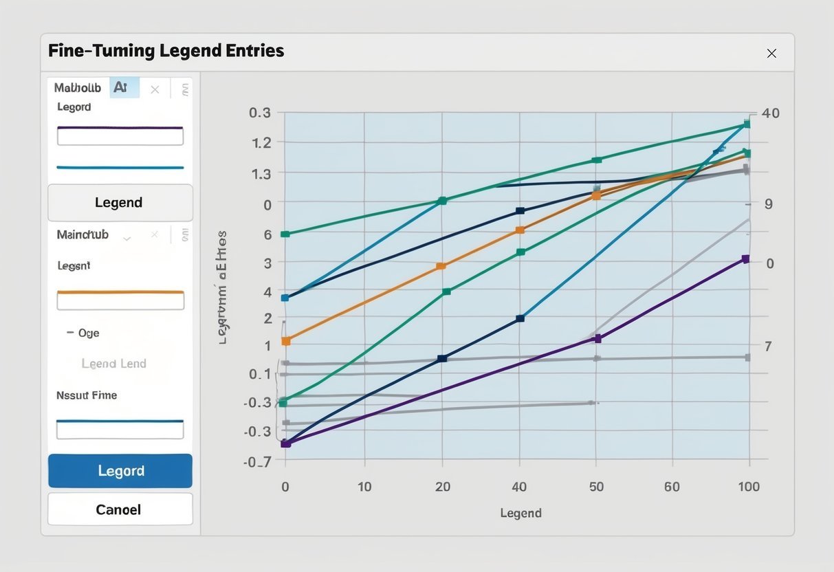
A graph with multiple lines and corresponding labels, demonstrating the process of fine-tuning legend entries in Matplotlib

Fine-tuning legends in Matplotlib is essential for clear data presentation. Adjustments can be made to the order of items and the appearance of markers and lines, enhancing plot readability.

Setting the Order of Legend Entries

In Matplotlib, controlling the order of legend entries can simplify plot interpretation.

By specifying the legend_labels parameter, users can decide which data series appear in the legend. The set_label method allows for customizing the labels of individual plot elements.

To display certain entries first, use numpoints to control marker repetition within the legend.

Arranging markers with markerfirst either before or after the label offers flexibility in display order. When necessary, a manual legend can be crafted for fine-tuned control.

Customizing Markers and Lines

Customizing markers and lines in legend entries is crucial for enhancing visual appeal.

The legend_labels parameter helps specify which plot items should be included and how they should appear.

Various styles, such as dashed or solid lines, can be assigned to different data series.

Markers can be adjusted using the markerfirst parameter to position before or after the text. The frameon option allows toggling of the legend’s border for better readability. Through detailed adjustments, the legend becomes not only informative but also visually coherent.

Frequently Asked Questions

A computer screen displaying a line graph with a stylized legend, surrounded by open books and a pen

Matplotlib offers many styling options for customizing legends. Understanding how to adjust the appearance, position, and formatting of legends can greatly enhance the readability and professionalism of plots.

How can one customize the appearance of the legend in Matplotlib plots?

Matplotlib provides many options for customizing legend appearance.

Users can change the legend’s font size, color, and style. Options also include adding borders or shadows. These customizations help make the information clear and matches the plot’s theme.

What methods are available for positioning the legend outside a Matplotlib plot?

Legends can be positioned outside the plot using the bbox_to_anchor parameter.

This allows users to manually place the legend at specific locations, like the top-right of a figure.

Adjusting the loc parameter provides several predefined positions, making it easy to achieve the desired layout.

Which parameters control the number of columns in a Matplotlib legend?

The ncol parameter in Matplotlib’s legend function allows setting the number of columns.

This is useful for arranging legend items in a more compact or spread-out manner, depending on the plot’s design and the number of entries.

How do you add and style a title for a legend in Matplotlib?

To add a title to a legend, use the title parameter within the legend function.

This title can be styled using font properties, such as font size and typeface. Styling options make the legend title prominent, enhancing plot clarity.

What are the options for adjusting the font size of legend text in Matplotlib?

The fontsize parameter in the legend function allows users to change the size of the legend text.

This can be a specific size or a string value like ‘small’, ‘medium’, or ‘large’, offering flexibility to fit different plot sizes and styles.

Can you provide an example of configuring the border and background of a legend in Matplotlib?

To configure a legend’s border and background, use parameters like frameon, edgecolor, and facecolor.

For example, setting edgecolor changes the border color, while facecolor adjusts the background color.

This customization adds a professional touch to the plot, ensuring the legend stands out appropriately.

Categories
Uncategorized

Learning T-SQL – Query and Manage XML Data Strategies Explained

Understanding XML Data in SQL Server

In SQL Server, XML data can be managed effectively with specific data types and schema collections.

Knowing the basics of XML data types and how to use XML Schema Definitions (XSD) can enhance data handling in SQL environments.

Basics of XML Data Type

The XML data type in SQL Server allows users to store and query XML formatted data. This data type offers great flexibility for handling semi-structured data within a relational database system.

Users interact with XML data using server functions like XMLNODE, XMLQUERY, and XMLVALUE. These functions help parse and manipulate the data easily.

The XML data type supports methods to extract data, transform it, and even validate the structure to ensure it matches expected patterns.

Utilizing the XML data type improves data interchange between SQL Server and various applications. It is crucial for scenarios where the data generated or consumed needs to be in a hierarchical format rather than a flat, tabular structure.

This is particularly beneficial for data exchange in web services and applications requiring complex data structures. In short, it allows seamless integration of XML formats with relational data.

XML Schema Collection and XSD

XML Schema Collection in SQL Server serves as a container for one or more XML Schema Definitions (XSDs). This collection helps validate XML data stored within an XML column, ensuring that XML documents meet specific structural and data requirements. This process improves data integrity and reliability.

When XML data is inserted, the server uses the XSD to check for compliance with defined rules. This validation process makes sure that the XML data adheres to predetermined formats and constraints, akin to data validation in traditional databases.

The schema collection reduces overhead in repeated validation, helping maintain performance efficiency. It is instrumental in environments where structured data modeling is critical.

By using XML Schema Collections, users can manage complex data more effectively and enforce strict data integrity rules. This capability ensures that XML data remains consistent, accurate, and reliable over time.

Working with the T-SQL Query Language

T-SQL is a powerful tool for working with XML data. It provides functions and methods like query(), value(), exist(), modify(), and nodes() to query and manipulate XML within SQL Server. These capabilities make it easier to manage complex data formats.

Introduction to T-SQL for XML

T-SQL offers robust support for handling XML data. One vital feature is the ability to query XML data using T-SQL’s specialized methods.

The query() method retrieves fragments of XML, allowing detailed data extraction. The exist() method checks for the presence of specific nodes or values, enhancing conditional logic within queries.

Through the modify() method, users can alter XML content directly within the database, improving workflow efficiency.

These methods work together to provide comprehensive XML manipulation directly within SQL Server, facilitating smooth data management for developers.

T-SQL’s integration of these XML features allows precise operations, ensuring that developers can extract, verify, and update XML data efficiently.

Utilizing the Value() Method

The value() method in T-SQL is used to extract values from XML data as SQL types, enhancing the ability to work with different data formats. This method converts XML nodes or attributes into scalar values, which can then be easily handled within SQL queries.

For example, when combined with the nodes() method, value() enables the extraction and use of specific XML values for calculations or data transformations.

By leveraging the value() method, developers ensure that their applications can efficiently translate XML data into usable formats, streamlining both data retrieval and processing within SQL environments.

Executing Basic XML Queries

When working with XML data in T-SQL, it’s essential to understand how to query XML and use the FOR XML clause effectively. These tools allow for the retrieval and management of XML data stored in SQL Server.

Using the Select Statement

The SELECT statement is crucial for querying XML data in SQL Server. It allows the user to extract specific data from XML nodes.

To retrieve information, one can use the value() method, which extracts the value of a single node in the XML data. The nodes() method is used to define how the XML data is shredded into rows.

Inline functions like OPENXML, XQuery, and XMLTABLE simplify data retrieval.

For example, SELECT with XQuery expressions can query XML documents directly, making it easier to handle complex hierarchical data structures.

With these tools, users can perform precise and efficient queries on XML data stored within SQL databases.

Employing the For XML Clause

The FOR XML clause is a powerful feature in T-SQL, used to convert SQL query results into XML format. This is particularly useful when transferring data between systems that support XML well.

There are different modes available such as RAW, AUTO, EXPLICIT, and PATH, each offering unique ways to structure the XML output.

The RAW mode produces a simple, element-centered XML tree, while AUTO creates nested XML by automatically identifying the hierarchy from the table relationships.

In more complex scenarios, PATH provides greater customization by allowing users to define the XML structure explicitly.

Through these modes, SQL Server users gain robust flexibility in creating XML documents from query results.

Advanced Query Techniques

When working with T-SQL to handle XML data, advanced techniques like XQuery and the Cross Apply function provide powerful tools. These methods enhance querying efficiency and allow for detailed manipulation and analysis of XML data within SQL Server.

Leveraging XQuery in SQL Server

XQuery is a robust language for querying XML data. It is integrated within SQL Server, enabling precise queries on XML instances. This allows users to extract, transform, and interact with XML directly within the database.

Using the query() method, developers can retrieve specific portions of XML data. This is essential for applications needing dynamic XML content manipulation.

For instance, selecting specific XML nodes or attributes can be achieved with a query like '//book/title', which targets the title elements within book nodes.

Utilizing XQuery expressions can significantly enhance database operations and efficiency, enabling complex querying and data retrieval directly from XML documents stored in SQL Server.

Its capability to handle hierarchical data structures makes it indispensable for applications with diverse and complex data needs.

Cross Apply for XML Nodes

The CROSS APPLY operator is crucial in SQL Server for accessing XML data more effectively. It works in conjunction with the nodes() method to transform XML data into a relational format, allowing for more straightforward querying and data manipulation.

When combined, CROSS APPLY and nodes() enable precise targeting of XML nodes. For example, retrieving node lists or performing operations on each node becomes seamless.

This is particularly useful when dealing with nested XML structures, as it allows for iteration over child nodes, extracting relevant data efficiently.

This approach streamlines accessing, transforming, and leveraging XML data, making it a valuable addition to any database handling complex XML data processing.

Integrating XML with Relational Data

A computer screen displaying XML code and a relational database table, with a person querying and managing the XML data using T-SQL

Integrating XML data with a relational database involves processes that allow seamless query and management of data. The main steps include transforming XML data into a relational format and effectively retrieving data using OpenXML functions.

Transforming XML to Relational Format

Transforming XML data into a relational format is a critical step for databases. XML files often have a complex hierarchy, making it necessary to map this structure into tables with rows and columns.

This is achieved by defining a schema that relates XML elements to database columns.

Tools like SQL Server let users import XML data, providing formats and tools for conversion. Using special data types designed for XML, users can store and query XML efficiently in relational databases.

Doing this ensures that the integrity of the XML data remains intact and query performance is optimized.

Many database systems offer built-in functions or methods to perform this transformation, making the process more straightforward for developers.

Retrieving Data with OpenXML

OpenXML is a crucial function used in SQL Server for reading XML data. It allows users to work with XML data as if it were a database table.

By parsing the XML document, OpenXML can select and retrieve data efficiently from within the file.

First, an XML document is prepared, and OpenXML is initialized. When the function is executed, it converts XML into a rowset that mirrors table rows.

This makes it simple to query and join XML data with traditional tables.

Using OpenXML in SQL Server provides flexibility in handling XML data, allowing complex data operations without needing to transform XML into another format first.

This function is particularly powerful for developers dealing with dynamic or nested XML structures.

Managing XML Variables and Data Models

Managing XML variables and data models in T-SQL involves handling XML type variables and leveraging XML for effective data organization. It details the creation of XML data instances and the design of models that can store and retrieve structured data efficiently.

Defining XML Type Variables

XML type variables allow T-SQL users to store and manipulate XML data within SQL Server. When defining an XML type variable, it is important to declare it correctly to ensure that it can handle the expected XML document structure.

These variables are defined using the xml data type in SQL Server.

For example, to declare an XML variable named @xmlData, one can use the following syntax:

DECLARE @xmlData xml

This variable can then be assigned XML values and queried for data extraction.

It allows users to create instances of XML data, manipulate them, and query specific nodes or attributes. Proper use of XML variables enables efficient storage and retrieval of structured data within SQL databases.

They offer flexibility in handling both small snippets and large XML documents.

Designing Data Models Using XML

XML data models offer a structured approach to managing complex data. By using XML, it is possible to create rich, hierarchical data relationships that are easy to navigate and query.

This design is beneficial when dealing with data that naturally fits into a tree structure, such as catalogs or configuration settings.

The process involves defining the structure of the XML document, which serves as the model. This model specifies how data is organized in terms of elements, attributes, and nesting, providing a clear blueprint for data storage and retrieval.

Additionally, with the use of T-SQL capabilities, developers can query and manipulate XML nodes, supporting a wide range of applications.

Models can be used to validate the structure of XML data before insertion into the database, ensuring data integrity and consistency.

This approach allows for dynamic and adaptable data models, greatly enhancing the flexibility and scalability of the database systems.

Utilizing XML Namespaces

Using XML namespaces in T-SQL allows developers to effectively organize and manage XML data. Learning how to use these namespaces is crucial for handling XML documents correctly, especially when dealing with attributes and elements that might have the same names but different meanings.

Understanding Namespaces and Prefixes

XML namespaces are identifiers that differentiate elements or attributes with the same name but different contexts. They prevent confusion and collisions by providing a unique namespace URI.

Prefixes act as shorthand for these URIs. For example, xmlns:ex="http://example.com/schema" declares a namespace prefix ex. This allows developers to reference XML elements like <ex:item> clearly linked to the declared namespace.

Singletons, in this context, refer to unique attributes or elements defined within that namespace. A carefully chosen prefix helps maintain readability and access specific XML content without ambiguity.

Querying with XMLNamespaces

The WITH XMLNAMESPACES clause in T-SQL is used to declare the XML namespaces that are needed for a query. By defining prefixes, developers can extract and manage data accurately from XML documents.

Consider a query designed to select XML data with specific namespaces. It uses the WITH XMLNAMESPACES clause to assign prefixes, ensuring elements like <ex:item> are correctly parsed.

When querying, these prefixes help avoid errors and ensure the correct elements are retrieved. The query syntax typically involves brackets to specify the desired elements, using the prefixes defined in the XML namespaces clause to streamline the access process to the structured XML content.

Working with Typed vs. Untyped XML

Typed and untyped XML have different uses and benefits when working with database systems. Typed XML is associated with an XML Schema (XSD), providing more structure and validation. Meanwhile, untyped XML is more flexible and can hold any XML content without strict data type definitions.

Differences Between Typed and Untyped XML

Typed XML is linked to an XML Schema (XSD), which defines the structure, elements, and data types. This enables strong validation and data integrity by ensuring that XML documents adhere to a predefined format. Using typed XML means the database can enforce these rules whenever data is inserted or modified.

In contrast, untyped XML is not tied to any schema, allowing for greater flexibility but sacrificing the strict validation that typed XML provides. As a result, untyped XML can store a wide range of XML documents without checking for specific data types or structures. This can be useful in scenarios where data structures might change frequently or are not predefined.

Implementing Typed XML

To implement typed XML, define an XSD that describes your data model. This schema includes details about the XML format and the types of data each element or attribute can contain.

Once the schema is defined, it is linked to the XML data type column in SQL Server. This setup allows T-SQL to use various XML data type methods for querying and modifying XML content.

These methods include query(), value(), exist(), and nodes(), enabling efficient data manipulation. By enforcing typed XML, it ensures compliance with the schema on both function calls and data operations. Typed XML is ideal for scenarios requiring strict data consistency and validation.

Manipulating XML Data with T-SQL

Manipulating XML data with T-SQL involves using methods like modify() and nodes() to efficiently handle XML instances. These methods allow developers to update, insert, or delete XML nodes, as well as navigate through complex XML structures, enabling streamlined data management tasks.

Using Modify() Method in XML

The modify() method is a crucial tool for altering XML data directly within SQL Server. It allows a user to update, insert, or delete XML content in an XML column. This method uses XML DML (Data Manipulation Language) expressions to perform its functions.

For updates, the modify() method can replace existing values within an XML instance. For example, changing a specific node value requires an update expression. Insertion is handled by specifying a node and the position where new data should be inserted. Deletions involve selecting the appropriate node to remove, which helps maintain the structure without affecting other data. Mastering the modify() method can significantly enhance efficiency when working with XML data.

Handling XML Nodes with Nodes() Method

The nodes() method is essential for breaking down XML data into a form that can be queried more easily in T-SQL. It allows the conversion of complex XML structures into row sets, which can then be queried using regular SQL statements.

By using the nodes() method, developers can extract specific parts of the XML for detailed querying. This method assigns the XML nodes to a table structure, making it possible to navigate through each node systematically. Converting XML to row data enhances readability and analysis, particularly when dealing with large XML documents. The ability to handle individual nodes efficiently through the nodes() method simplifies XML data management and query processes.

Incorporating XML Data into Azure SQL

Integrating XML data into Azure SQL involves understanding both Azure SQL Database and Azure SQL Managed Instance. With XML, you can handle hierarchical data effectively and Azure SQL offers robust support for this.

Azure SQL Database and XML

Azure SQL Database allows users to store, query, and manage XML data seamlessly. XML data types can be used for storing XML documents, enabling complex data structures to be embedded within database tables. Users can employ XQuery for querying XML data, providing flexible ways to retrieve and manipulate hierarchical information.

Moreover, T-SQL functions like query(), value(), and exist() help in extracting data from XML documents. Developers may also use xml.modify() for updating XML instances stored in the database. Designing the schema ensures efficient data processing when dealing with XML files.

Azure SQL Managed Instance Considerations

Azure SQL Managed Instance shares many features with Azure SQL Database, but there are some additional considerations. This service supports cross-database queries, which is advantageous when dealing with XML data across multiple databases. Additionally, it provides integrated security features that safeguard XML data transactions.

Managed Instance also supports SQL Server Agent for scheduling jobs, making batch processing of XML data more efficient. It’s important to handle XML namespaces correctly when storing and retrieving XML data to avoid conflicts and ensure data integrity. Proper setup facilitates smooth integration of XML files and data streams.

XML Data Import and Export

When working with XML data in SQL Server, it is crucial to know how to effectively import and export data. This involves techniques for pulling XML data into the database and exporting it in useful formats.

Importing Data Using OpenRowset and Bulk

OpenRowset is a versatile function in SQL Server that enables data import from various sources. For XML data, it’s used to read data from a file and insert it into a table. The syntax often includes specifying BULK along with the file path to load the XML content.

For instance, using OpenRowset with a bulk option allows loading XML data efficiently in one batch. This method does not require creating a linked server and is useful for ad-hoc access.

sp_xml_preparedocument can also be utilized for parsing XML data. This stored procedure takes an XML document into a local variable, making it easier to work with in queries. After importing, data can be queried and inserted into tables for further analysis and management.

Exporting Data with For XML

The For XML clause in SQL Server is a powerful tool for exporting data as XML. When appended to a SELECT statement, it formats the result set as XML. This is useful for creating XML documents from database tables.

Using the PATH mode in For XML gives fine control over XML formatting, allowing custom structuring of the output. This clause is essential for applications needing XML-formatted output, making data easily shareable across different systems.

To efficiently export large data sets, batch processing can be applied. Exporting in smaller chunks prevents exceeding limits and ensures smoother performance.

Maintaining XML Data Integrity

A computer screen displaying a T-SQL query code manipulating XML data with a focus on data integrity

Ensuring the accuracy and consistency of XML data is vital in databases. This involves working with various tools and techniques to guarantee that XML data is well-formed and valid according to defined schemas.

Working with XML Schema Collections

An XML Schema Collection is a database object that holds XML schemas. These schemas define the structure and rules for XML documents stored in a database.

By using a schema collection, you can enforce constraints on XML data, ensuring it meets specific requirements for structure and data types. This process helps in maintaining the integrity of the data.

Adding schemas to a collection involves using Transact-SQL commands. Once defined, the schemas in the collection help validate incoming XML data, ensuring it adheres to the predefined structure before it’s stored. This approach minimizes errors and enhances consistency across XML documents.

Learn more about defining data integrity using schemas in Transact-SQL.

Cleaning Up with SP_XML_RemoveDocument

The sp_xml_removedocument procedure in SQL Server is used to free memory resources by cleaning up the XML documents stored in memory.

When XML data is opened using sp_xml_preparedocument, memory is allocated for handling the XML content. To avoid memory leaks and optimize performance, it is crucial to use sp_xml_removedocument once you finish with the XML processing.

This procedure accepts a handle to the document and releases the resources associated with that handle. Effective use of sp_xml_removedocument is important for maintaining system performance and preventing resource wastage. Proper management of these documents ensures that the server can efficiently handle concurrent XML processing tasks without degradation.

Explore the management of XML features and T-SQL queries on SQL Server.

Frequently Asked Questions

Working with XML data in SQL Server involves parsing, generating output, and converting data effectively. Knowing these processes helps manage and query XML data efficiently.

What are the steps to parse XML data within SQL Server?

To parse XML data, one can use the nodes method to break down XML into a rowset. The value method extracts data from XML nodes. Using these methods together allows effective navigation through XML structures in SQL Server.

How can you generate XML output from a SQL query?

Generating XML output involves using the FOR XML clause in SQL Server queries. This clause can be added to a SELECT statement to format the result set as XML. Options like RAW, AUTO, and PATH determine the structure of the output.

What is the process for converting XML data into a SQL query?

Converting XML data into a SQL query can be achieved with the OPENXML function. This function, along with the sp_xml_preparedocument stored procedure, allows SQL Server to read and execute queries on XML data as if it were a table.

In what ways can SQL Server read XML files?

SQL Server can read XML files by using OPENROWSET or BULK INSERT to import data from an XML file into a database table. Another way is through the XML data type, which can store and query XML data directly.

Can you provide examples of querying XML data with SQL Server?

Examples of querying XML data include using the XQuery language to extract XML node values. The query and exist methods allow retrieval and checking for specific nodes or values, helping users access and manipulate XML content.

What methods are available for the fast parsing of XML in SQL Server?

Fast parsing of XML can be optimized with techniques like using indexes on the XML column. The nodes method can also be used to split large XML documents. Additionally, limiting the XML content processed in queries can enhance performance.

Categories
Uncategorized

Learning about Linear Regression – Mastering Ordinary Least Squares Techniques

Fundamentals of Ordinary Least Squares (OLS)

Ordinary Least Squares (OLS) is a key technique in linear regression that helps estimate the linear relationship between variables.

Its primary goal is minimizing the differences between observed and predicted values, ensuring the best fit line for data.

Understanding the OLS Method

Ordinary Least Squares is a statistical method used to estimate the coefficients in a linear regression model.

It works by minimizing the sum of the squared residuals, which are the differences between observed values and the values predicted by the model. This process results in a line that best fits the available data.

OLS assumes linearity, meaning the relationship between the dependent variable and each independent variable is linear.

Additionally, it requires that errors, or residuals, are normally distributed and have constant variance. These assumptions are crucial for ensuring accurate and reliable results.

If these conditions are met, OLS provides unbiased and efficient estimates of the coefficients, allowing for meaningful interpretation and predictions.

The Heart of Linear Regression

At the core of linear regression, OLS determines how changes in independent variables affect the dependent variable.

By calculating the equation of a straight line, OLS finds the optimal fit by adjusting the coefficients. These coefficients quantify the effect each independent variable has on the dependent variable, helping to understand how different factors contribute to variations in the outcome.

The resulting regression line reveals patterns and trends within data while highlighting the strength of the relationship between variables.

Practically, this means making accurate forecasts and data-driven decisions becomes possible across various domains, from economics to biology.

The effectiveness of OLS hinges on proper application and adherence to its assumptions, ensuring robust and applicable findings in real-world scenarios.

Key Concepts and Terminology

Understanding linear regression involves grasping a few essential concepts. These include the roles of dependent and independent variables, as well as the function of coefficients and intercept in predicting outcomes.

Defining Dependent and Independent Variables

In a linear regression model, the dependent variable represents the outcome or the variable we aim to predict. It is typically denoted as ( y ).

The independent variables, on the other hand, are the predictors or inputs. They are often represented as ( x_1, x_2, ldots, x_n ), and affect the dependent variable. These variables can be manipulated to see how changes impact the dependent variable, making them crucial for model accuracy.

In practical terms, if one wanted to predict house prices (dependent variable), features such as location, size, and number of rooms are independent variables. By analyzing how these inputs affect price, more accurate predictions can be made.

Exploring Coefficients and Intercept

Coefficients in a linear regression model measure the relationship between each independent variable and the dependent variable.

These values tell us how much the dependent variable is expected to change when the independent variable changes by one unit.

The intercept represents the constant term in the equation. It indicates the expected value of the dependent variable when all independent variables are zero.

In the equation ( y = b_0 + b_1x_1 + b_2x_2 + ldots + b_nx_n ), ( b_0 ) is the intercept, and ( b_1, b_2, ldots, b_n ) are the coefficients.

These elements form the crux of the regression equation, revealing insights about data relationships. Proper estimation and interpretation are key to model success, impacting the predictions generated by the regression analysis.

Assumptions Behind OLS

Ordinary Least Squares (OLS) regression relies on several key assumptions to produce reliable estimates. Key assumptions include linearity, independence, homoscedasticity, and normality. Violating these assumptions can lead to biased results or inefficient estimates.

Linearity and Independence

The assumption of linearity means that the relationship between the independent variables and the dependent variable should be linear. This implies that changes in the independent variable are associated with proportional changes in the dependent variable.

It’s essential to check for linearity since non-linear relationships can lead to incorrect model predictions.

Independence is another critical assumption. Observations should be independent of each other—meaning that the outcome of one observation does not affect another.

Independence helps ensure that the sample provides a true picture of the population. Dependence between observations can result in unreliable estimates and increase the chance of Type I or Type II errors.

Homoscedasticity and Normality

Homoscedasticity refers to the constant variance of residuals, or errors, across all levels of the independent variable.

In OLS, it’s crucial that the spread of these errors remains consistent as different independent variable values are encountered. If the model shows signs of heteroscedasticity, or non-constant variance, it may affect the accuracy of coefficient estimates and predictions.

Normality assumes that the residuals of the model are normally distributed. This condition is important for hypothesis testing and estimating confidence intervals.

If residuals do not follow a normal distribution, it might suggest the need for data transformation or the use of alternative estimation methods. This assumption is particularly vital when conducting t-tests or deriving statistical inference from the model.

Building the Regression Model

Creating a regression model involves specifying the model and determining the best-fit line that suits the data. The process includes choosing the right variables and methods to find the best parameters that satisfy the linearity assumption.

Model Specification and Selection

Selecting the right model is crucial in building a regression model. This step involves deciding which variables to include as predictors and ensuring that they effectively capture the relationship with the dependent variable.

It’s essential to check the linearity assumption to ensure that a straight line can approximate the data accurately. Researchers often assess various models, comparing them using criteria like R-squared, AIC, and BIC to determine the best fit.

The chosen model should minimize the error between observed and predicted values. This trade-off between simplicity and accuracy is key to model selection.

Calculating the Best-Fit Line

Once the model specification is complete, the next step is calculating the best-fit line.

This involves using techniques like Ordinary Least Squares (OLS) regression to estimate the model parameters.

OLS minimizes the sum of squared differences between observed and predicted values, ensuring the line is as close as possible to the data points.

By finding the optimal slope and intercept, the regression model aligns well with the data trends. Calculating these parameters accurately is important, as they indicate the strength and direction of the relationship. A precise best-fitting line helps make reliable predictions and draw meaningful insights from the data.

Regression Analysis and Interpretation

Regression analysis is a powerful tool in statistics, used to understand the relationship between variables. Key components include the sum of squared residuals and R-squared values, which help in interpreting how well a model fits the data.

Investigating the Sum of Squared Residuals

The sum of squared residuals (SSR) is a measure of how well a regression line fits a set of data points. It calculates the total squared differences between the observed values and the values predicted by the model.

A lower SSR indicates a better fit, as it suggests that the data points are closer to the regression line.

In regression analysis, minimizing the SSR is crucial because it helps find the best-fitting line through the data. The Ordinary Least Squares (OLS) method specifically focuses on this by aiming to make the SSR as low as possible.

Analysts can assess model accuracy by examining the SSR, with lower values indicating more reliable predictions.

Residuals are vital in checking if assumptions of linear regression are met. If they show non-random patterns, it may indicate issues such as non-linearity or heteroscedasticity.

Understanding R-Squared and Adjusted R-Squared

R-squared is a statistical measure that indicates how much of the variance in the dependent variable can be explained by the independent variables in the model.

It ranges from 0 to 1, where a higher value signifies a better fit of the model to the data.

While R-squared gives an idea of fit, it may be misleading when adding more variables to the model. This is where adjusted R-squared becomes useful.

It adjusts the R-squared value for the number of predictors, providing a more accurate measure when multiple independent variables are involved.

Adjusted R-squared is essential when comparing models with different numbers of predictors. It can help prevent overfitting by showing whether additional variables improve the model’s performance significantly or not.

OLS Estimation Techniques

Ordinary Least Squares (OLS) estimation is a method used to find the best-fitting line in linear regression analysis. The aim is to minimize the differences between observed values and estimated values. Two primary techniques for implementing OLS include using the Statsmodels library in Python and understanding the role of gradient descent.

Utilizing Statsmodels and Python

Statsmodels is a powerful Python library that simplifies statistical modeling.

It offers a user-friendly interface for conducting OLS estimations. By incorporating Statsmodels, users can easily estimate OLS coefficients with functions like OLS() and fit().

Statsmodels also provides summary tables that display these estimators and additional statistics. These tables include R-squared values, coefficients, and standard errors, making them an essential tool for analysts.

Here’s a brief example of how OLS estimation works in Statsmodels:

import statsmodels.api as sm

X = sm.add_constant(X)  # Adds a constant term to the predictors
model = sm.OLS(y, X).fit()
print(model.summary())

In this way, Statsmodels streamlines the process of performing OLS regression, enhancing clarity and accuracy. Python as a programming language supports versatile analytical processes, making it crucial for data scientists and statisticians.

The Role of Gradient Descent

Gradient descent is an optimization algorithm that iteratively adjusts model parameters to find the minimum value of a cost function.

In the context of OLS, this method can help refine model estimators when datasets are large or complex.

While traditional OLS directly calculates coefficients, gradient descent offers an alternative approach useful for machine learning models. It updates coefficients by taking small steps proportional to the gradient of the cost function.

Here is how the gradient descent algorithm typically functions:

  1. Initialize coefficients randomly.
  2. Compute the gradient of the cost function.
  3. Adjust the coefficients in the opposite direction of the gradient.
  4. Iteratively repeat until convergence.

This approach is especially valuable when dealing with large datasets or when computational efficiency is a priority. Gradient descent ensures precision and scalability while complementing the robust framework of linear regression analysis.

Challenges in OLS

Ordinary Least Squares (OLS) is a common method for estimating linear relationships. Challenges such as multicollinearity and outliers can impact model accuracy. These challenges require careful identification and handling to ensure reliable results.

Detecting Multicollinearity

Multicollinearity occurs when independent variables in a regression model are highly correlated. This can lead to unreliable coefficient estimates and inflate the variance.

One common way to detect multicollinearity is by calculating the Variance Inflation Factor (VIF). If the VIF value exceeds 10, it typically indicates a problem with multicollinearity.

Another method is examining the correlation matrix of the predictors. High correlation between two variables can hint at multicollinearity.

When multicollinearity is present, it becomes hard to determine the effect of each predictor on the dependent variable. One solution is to remove or combine correlated variables to improve model stability.

Addressing Outliers and Leverage Points

Outliers are data points that do not fit the trend observed in the rest of the data. Leverage points have an extreme value in an independent variable that can unduly influence the model’s estimates. Identifying influential points is crucial as they can distort the regression results.

One method to address outliers is to use graphical tools such as scatter plots to visualize data patterns.

Additionally, statistical tests can confirm the presence of outliers.

Robust regression techniques like L1 regression can help minimize the impact of outliers.

For leverage points, examining diagnostic plots such as Cook’s distance can be effective.

Removing or adjusting these points ensures more accurate and reliable regression results.

Properly managing outliers and leverage points helps maintain the integrity of OLS-based models.

Advanced OLS Concepts

Ordinary Least Squares (OLS) can be expanded into more advanced techniques. These include using weighted least squares to handle heteroscedasticity and employing regularization methods like lasso regression to improve model performance and interpretability.

Exploring Weighted Least Squares

Weighted Least Squares (WLS) is useful when the assumption of constant variance in errors, known as homoscedasticity, is violated. In such cases, variance in the data increases with some predictors.

WLS assigns different weights to data points during regression, accounting for varying reliability. This technique adjusts the loss function to minimize the mean squared error of the weighted errors.

By doing so, WLS can provide more efficient and unbiased estimates compared to traditional OLS.

Implementing WLS involves selecting appropriate weights for each data point, often inversely related to the variance of each observation.

This method ensures that OLS gives more emphasis to points with lower variance, thus stabilizing the variance and improving model accuracy.

Therefore, WLS is especially beneficial for data exhibiting heteroscedasticity.

Regularization with Lasso Regression

Lasso Regression introduces a penalty to the OLS model to prevent overfitting and enhance interpretability. The technique adds a regularization term to the loss function, encouraging the model to reduce complexity by driving some coefficients to zero. This exclusion of less important features simplifies the model while maintaining prediction accuracy.

Lasso modifies the traditional mean squared error criterion by including an absolute value penalty of the coefficients.

Mathematically, the objective is to minimize this penalized loss function, allowing the model to handle multicollinearity.

While similar to other regularization methods, lasso excels in situations where many predictor variables hardly contribute to the desired outcome.

Selecting important features becomes straightforward, making models easier to interpret and improving generalization to new data.

Practical Applications of OLS

Ordinary Least Squares (OLS) is widely used in several fields to analyze relationships between variables. It helps in understanding complex data patterns and predicting future trends, which is crucial in both finance and public services like healthcare and education.

In Finance and Econometrics

In the world of finance, OLS is an essential tool for evaluating asset pricing models and understanding market behavior. Analysts use OLS to estimate the returns and risks of various financial assets. Using historical data, it enables predicting stock prices, bond yields, and foreign exchange rates.

In econometrics, OLS is used to study economic relationships and forecast economic variables. It helps in determining the impact of factors like interest rates and inflation on economic growth.

Economists rely on OLS to model and test hypotheses about economic theories and to improve policy making.

Applications in Healthcare and Education

In healthcare, OLS models can identify patterns in patient data to improve treatment outcomes. Researchers use it to examine the effects of different variables like age, lifestyle, and medical history on health conditions.

This helps in making data-driven decisions about patient care and medical interventions.

In education, educators use OLS to analyze student performance data. It helps in identifying factors that influence academic success such as class size, teaching methods, and socio-economic status.

By assessing these variables, schools can design more effective education strategies and policies to improve learning outcomes.

Evaluating Model Performance

A person studying a graph with a linear regression line, surrounded by equations and statistical data

Evaluating the performance of a linear regression model involves analyzing residuals and enhancing predictive abilities. Residual analysis and diagnostics help identify issues in model assumptions, while improving predictive power focuses on refining the model for better accuracy.

Residual Analysis and Diagnostics

Residuals are the differences between observed and predicted values in a dataset. Examining these residuals is crucial to check if a model’s assumptions hold true.

Residual analysis involves plotting residuals to see if they are randomly scattered, which indicates that the model assumptions are appropriate.

If patterns or structures appear in the residuals, this might suggest problems with model specification, such as missing variables or incorrect functional forms.

Diagnostics often include checking for normality of residuals, heteroscedasticity (non-constant variability), and autocorrelation (dependency between residuals).

Residual plots, such as scatter plots of residuals versus fitted values, are helpful tools. Histogram and Q-Q plots can further diagnose normality.

Addressing these diagnostic outcomes ensures that the model provides a reliable foundation for decision-making.

Improving Predictive Power

To improve a model’s predictive power, one should focus on refining model features and selecting appropriate variables.

Ensuring correct model specification involves including relevant predictor variables and interaction terms. Feature scaling and transforming non-linear relationships can also enhance predictive accuracy.

Another method to boost predictive power is through training-validation splitting. By separating data into training and validation sets, one can ensure the model generalizes well to new data.

Cross-validation is another technique that helps in assessing model consistency.

Regularization methods like Ridge or Lasso regression can prevent overfitting by penalizing complex models.

This balance helps in maintaining both simplicity and effectiveness in predictions.

Adjusting these aspects can notably increase the model’s precision and reliability over varying datasets.

Extending Beyond OLS

Ordinary Least Squares (OLS) serves as a foundation in linear regression. Exploring techniques like multiple linear regression and dimensionality reduction with Principal Component Analysis (PCA) allows for advanced analysis. These methods handle complex data sets and improve model accuracy.

Introduction to Multiple Linear Regression

Multiple Linear Regression (MLR) is an extension of OLS that considers multiple independent variables instead of just one. This technique is used when the relationship between dependent and independent variables is more complex.

By analyzing how each predictor variable influences the dependent variable, MLR can reveal intricate data patterns.

This method is vital in fields requiring multifactor analysis, such as finance and healthcare. MLR models can manage large amounts of data to provide deeper insights. Also, multicollinearity, where independent variables are correlated, can skew results. Regularization methods like Ridge and Lasso help mitigate this.

Dimensionality Reduction with PCA

Principal Component Analysis (PCA) is a key technique for dimensionality reduction. It simplifies data by transforming it into a set of uncorrelated variables called principal components.

PCA retains significant data variance, allowing for accurate modeling even with reduced dimensions.

This method is useful when dealing with high-dimensional data, such as genomics or image processing. PCA enhances computational efficiency and reduces overfitting by ignoring irrelevant features.

In statistical models, PCA aids in visualizing and interpreting complex datasets, making it easier to identify patterns and trends.

Technological Integration and Future Directions

A futuristic classroom with interactive screens displaying linear regression equations, while students engage in hands-on activities with data sets and graphs

As technology advances, Ordinary Least Squares (OLS) plays a crucial role in analyzing big data and machine learning models. These fields continuously evolve, utilizing OLS for its effectiveness in handling large datasets and capturing data patterns.

OLS in the Era of Big Data

In the age of big data, OLS remains a vital tool for uncovering relationships within large datasets. It helps identify significant variables by minimizing errors between observed and predicted values.

This optimization technique efficiently processes extensive data, offering insights into complex models.

Besides its basic applications, OLS can be integrated with other statistical tools. Combining OLS with techniques like dimensionality reduction improves efficiency and helps deal with the complexities arising from big data.

It enables more precise data analysis, essential for informed decision-making in data science.

Key Benefits:

  • Minimizes prediction errors
  • Works well with large datasets
  • Enhances model accuracy with integrated techniques

Machine Learning and OLS

In machine learning, OLS serves as a fundamental stepping stone for algorithm development. It’s particularly useful for linear models, providing a foundation for more advanced methods.

By minimizing squared errors, it ensures the predictive models align closely with actual data points.

OLS also supports deep learning models, aiding in training processes for neural networks. While not directly used in final models, it assists in understanding basic linear relationships before diving into more complex patterns.

Machine learning often integrates OLS with other techniques like regularization, which helps prevent overfitting by introducing penalties for larger coefficients.

This blend strengthens model performance, making OLS indispensable in developing machine learning strategies.

Frequently Asked Questions

A person at a desk studying a graph with a linear regression line, surrounded by books and notes

Ordinary Least Squares (OLS) is a central method in regression analysis, helping to derive the relationship between variables. It offers insights into estimation techniques and assumptions critical to its application. Various fields utilize OLS, demonstrating its broad relevance and versatility.

How is Ordinary Least Squares (OLS) utilized in regression analysis?

Ordinary Least Squares (OLS) is primarily used to estimate the parameters of a linear regression model. It works by minimizing the sum of squared residuals, which are the differences between observed and predicted values. This method yields a line that best fits the data.

Can you explain the difference between OLS and general linear regression?

OLS is a specific type of linear regression focused on minimizing squared differences. General linear regression can include additional variables and methods, such as those addressing distributions of errors or incorporating non-linear relationships.

While OLS is a basic approach, linear regression includes more complex variations.

What are the fundamental assumptions underlying the OLS method?

The OLS method relies on several assumptions: linearity, independence, homoscedasticity, and normality of the residuals. These assumptions ensure that the estimates are unbiased and consistent.

Violations of these assumptions might lead to inaccurate results.

How do you derive the OLS estimator formula?

The OLS estimator formula is derived through calculus and matrix algebra. It represents a mathematical approach to finding the parameter estimates that minimize the sum of squared differences between observed and predicted values.

The derivation process involves differentiating and solving for the coefficients.

What is the principle behind the OLS method in econometrics?

In econometrics, OLS helps quantify relationships among variables. It is used to infer causal relationships and predict outcomes by analyzing data from observations.

Economists often employ OLS to model and understand economic phenomena.

What are some practical examples where OLS regression is applied?

OLS regression is applied in various fields like economics, finance, and social sciences.

Examples include predicting housing prices, analyzing economic growth factors, and studying consumer behavior.

The method is widely used for its simplicity and effectiveness in modeling real-world data.

Categories
Uncategorized

Learning Data Scientist Roles: Navigating Essential Skills and Responsibilities

Understanding the Data Scientist Role

A data scientist is a data expert who plays a crucial role in analyzing and interpreting complex data to help organizations make informed decisions. They utilize statistical models, machine learning, and data visualization to solve problems and improve outcomes.

Data scientists have a strong background in mathematics, computer science, and domain-specific knowledge.

Key Responsibilities:

  • Data Analysis: Interpreting large datasets to identify trends and patterns.
  • Modeling: Developing predictive models to forecast future outcomes.
  • Communication: Presenting insights to stakeholders in a clear and concise manner.

The demand for data scientists is on the rise, making it an attractive career in data science. As organizations rely more on data-driven decisions, the need for skilled data scientists continues to grow.

To become a data scientist, individuals often pursue degrees in fields like computer science, statistics, or a related discipline.

Essential Skills:

  • Proficiency in programming languages, such as Python or R.
  • Expertise in statistics and machine learning algorithms.
  • Ability to use data visualization tools like Tableau or Power BI.

A data science career offers various roles and responsibilities, ranging from data analysis to algorithm development. The flexibility within the field allows data scientists to focus on areas that align with their interests and expertise.

The role of a data scientist is essential for businesses seeking to leverage data for strategic advantages. Their expertise enables organizations to harness the power of data, leading to smarter, data-informed decisions.

Educational Background and Skills

A data scientist at a desk surrounded by books, a computer, and various data visualization tools

Data science is a multidisciplinary field demanding both a strong educational foundation and versatile skills.

Critical areas for data scientists include mathematics and statistics, proficiency in programming, and familiarity with various tools and technologies.

Fundamental Knowledge in Mathematics and Statistics

Mathematics and statistics are the backbone of data science, providing the tools for data analysis and interpretation.

A strong grasp of statistics helps data scientists understand data distributions, variance, and probabilities. Skills in mathematics build the ability to model and solve complex problems.

Learning concepts like linear algebra, calculus, and statistical inference is crucial. These areas help in developing algorithms and performing data manipulation tasks.

R and Python are popular languages for statistical analysis, offering libraries that support vast statistical functions and data visualization. This foundation is essential for making informed decisions based on data insights.

Programming Proficiency

Programming is vital for data manipulation, analysis, and model building in data science.

Python and R are widely used due to their flexibility and extensive libraries, such as NumPy and pandas. These tools allow data scientists to automate tasks and handle large datasets efficiently.

SQL is another key language, enabling data scientists to retrieve and manage data in databases.

Additionally, understanding Java and other programming languages can be beneficial for building data-driven applications.

Programming skills also facilitate the integration of machine learning algorithms to predict outcomes and trends.

Diverse Data Science Tools and Technologies

Data scientists use a vast range of tools and technologies to manage and analyze data.

Familiarity with data visualization tools like Tableau and libraries in Python (e.g., Matplotlib and Seaborn) is important for presenting data insights.

Machine learning frameworks like TensorFlow and sci-kit-learn allow for model building and deployment.

Knowledge of data science tools enhances productivity by simplifying processes, from data cleaning to model evaluation.

Mastery of cloud platforms like AWS or Google Cloud is increasingly valuable, providing scalable computing resources and storage solutions for handling big data effectively.

Specialized Knowledge in Machine Learning

Understanding the specific skills required for a role in machine learning is crucial. These roles often demand a strong grasp of core algorithms and advanced artificial intelligence techniques, including deep learning frameworks like TensorFlow and PyTorch.

Core Machine Learning Algorithms

Core machine learning algorithms form the backbone of predictive modeling. They include techniques such as linear regression, decision trees, and support vector machines.

These algorithms help machines learn from data, recognize patterns, and make decisions.

Tools like scikit-learn are popular for implementing these algorithms. They provide efficient implementations of algorithms for classification, regression, clustering, and more. Mastery of these tools allows data scientists to build models that analyze and predict outcomes effectively.

Understanding these algorithms includes knowing when to apply each one. For instance, decision trees are intuitive but may overfit; support vector machines are powerful but computationally intensive. Thus, knowing the strengths and weaknesses of each algorithm is key to success in machine learning roles.

Advanced Techniques in AI and Deep Learning

Advanced techniques in AI and deep learning go beyond traditional machine learning. They involve neural networks, including convolutional and recurrent networks, which are essential for complex tasks like image recognition and language processing.

Frameworks such as TensorFlow and PyTorch are widely used in this field.

TensorFlow offers scalability, while PyTorch is known for its dynamic computation graph, which simplifies building neural networks.

These tools enable the development of sophisticated AI models capable of handling massive datasets and performing intricate tasks.

Proficiency in deep learning requires an understanding of how these networks learn and adapt.

This includes concepts like backpropagation, activation functions, and optimization algorithms.

The ability to work with these advanced techniques is essential for those aiming to specialize in AI roles within data science.

Data Management Capabilities

A data scientist analyzing and organizing data with various tools and techniques

Data management capabilities are essential in the role of a data scientist. These capabilities involve both handling data efficiently and designing architectures for data deployment. Mastery of these skills ensures that data scientists can manipulate and analyze large datasets while effectively implementing system architectures.

Expertise in Data Manipulation and Analysis

Data manipulation and analysis are at the core of a data scientist’s role.

Proficiency in data manipulation involves cleaning and transforming raw data to make it usable for further analysis. This process includes filtering, aggregating, and restructuring data.

Analysis requires statistical techniques to extract insights from data. Data scientists often use languages like Python or R to write scripts for analysis.

It’s crucial to understand big data technologies such as Hadoop and Spark, which allow processing large datasets efficiently. These tools support large-scale computations and data storage, facilitating deeper insights.

Deployment and Architectural Design

Deployment and architectural design are vital for implementing data solutions. This involves creating robust systems to support data processing and accessibility.

Data architects design frameworks that manage data flow and storage, ensuring stability and scalability.

Data engineering plays a key role in building pipelines for data collection and warehousing. With big data growing in importance, specialists use modern technologies to optimize data processing systems.

Hadoop and Spark are commonly used for their ability to handle vast amounts of data efficiently, making these technologies essential for both deployment and architecture in data management systems.

Skills in Data Visualization and Business Intelligence

A data scientist visualizing business intelligence data using charts and graphs

Mastering data visualization and business intelligence skills is essential for data scientists. These abilities not only involve creating engaging visual representations of data but also extracting valuable insights to drive decision-making.

Creating Impactful Data Visualizations

Creating effective data visualizations is crucial for translating complex data into understandable insights.

It involves using tools like Tableau and Power BI to design charts and graphs. These tools help display patterns, trends, and outliers in a dataset clearly and concisely. The choice of visualization type, such as bar graphs for comparisons or line charts for trends, directly impacts understanding.

Skills in data storytelling enhance the communication of these visuals to a wide audience. Data scientists must focus on clarity and precision, ensuring that visualizations are accessible and informative.

Leveraging BI for Data Insights

Business Intelligence (BI) tools play a pivotal role in analyzing data to uncover actionable insights.

Power BI and Tableau are popular choices, offering features for data modeling, reporting, and dashboard creation. These tools enable users to identify key performance indicators and track business metrics effectively.

A strong grasp of BI involves not just technical ability but also strategic thinking to align data insights with business goals.

Data scientists use these insights to inform business strategies, improve operations, and forecast future trends. Integrating these skills into daily workflows can significantly boost a team’s effectiveness in decision-making processes.

Roles of Communication and Collaboration

A group of diverse individuals working together, sharing ideas and information, using technology to analyze and interpret data

Effective communication and collaboration are essential skills for data scientists. They help bridge the gap between complex data and practical solutions.

Communication involves translating data findings into clear insights. Data scientists must present their findings in a way that non-technical colleagues can understand. This skill is crucial when addressing business problems effectively.

Collaboration means working with different teams, often in interdisciplinary settings.

Successful collaboration requires the ability to share ideas and adapt to varying work styles. This can lead to creating more impactful solutions by leveraging interdisciplinary expertise.

Data scientists often bring business acumen to their roles by interpreting data in ways that align with business goals. This requires understanding the company’s objectives and tailoring data applications to fit these needs.

Leadership qualities are often needed when guiding teams through data-driven decisions.

By effectively communicating findings and recommendations, data scientists can influence pivotal business strategies. Building strong leadership abilities fosters trust with stakeholders and encourages collaborative efforts.

Data Science Methodologies

A scientist surrounded by data charts and graphs, studying various methodologies for data science

Data science methodologies involve systematic approaches to extract insights from data. Key aspects include statistical techniques and predictive models, as well as initial data investigations and feature creation for analytical success.

Statistical Analysis and Predictive Modeling

Statistical analysis serves as the backbone of data science, allowing practitioners to discern patterns and draw informed conclusions from data.

Techniques such as regression analysis, hypothesis testing, and correlation coefficients are regularly used. These tools help in understanding relationships between variables.

Predictive modeling employs these statistical techniques to forecast future outcomes.

It leverages algorithms like linear regression, decision trees, and neural networks. By examining past data, these models generate predictions about future events, driving decision-making processes.

Exploratory Data Analysis and Feature Engineering

Exploratory Data Analysis (EDA) is pivotal in the data science workflow. It involves summarizing main characteristics of data using visualizations and initial analyses without complex models.

Techniques like box plots, histograms, and scatter plots help uncover underlying patterns, spot anomalies, and test hypotheses using simple visual cues.

Feature engineering follows EDA and involves transforming raw data into informative features. This process significantly improves model performance.

Techniques include scaling, encoding categorical variables, and extracting time-based features. Effective feature engineering refines raw data inputs, enhancing predictive accuracy and facilitating the efficient functioning of machine learning models.

Problem-Solving and Critical Thinking

A data scientist pondering over complex algorithms and problem-solving techniques, surrounded by charts, graphs, and computer screens

Problem-solving and critical thinking are essential skills in data science. They enable professionals to analyze complex data sets and extract meaningful insights.

A data scientist must efficiently break down complex tasks into manageable parts, as described in the process of problem decomposition.

Critical thinking involves evaluating data from various angles. This helps in making informed decisions. Data scientists often rely on critical thinking to assess data quality and choose the right analytical methods.

Skills Overview:

  • Problem-Solving: Involves breaking challenges into smaller, manageable parts and finding solutions systematically.

  • Critical Thinking: Focuses on analyzing the credibility of data and its implications.

A strong foundation in data analytics allows data scientists to create predictive models. These models are crucial for forecasting trends and making data-driven decisions.

The ability to interpret data correctly is key to developing accurate predictions.

Tools and Techniques:

  • Data Analytics: Used for interpreting large volumes of data.

  • Predictive Models: Created to forecast future outcomes based on historical data patterns.

Effective communication of data insights is also vital. Data scientists must convey complex information in an understandable way.

This skill ensures that different stakeholders can act on the findings efficiently, supporting the company’s strategic goals.

Career Tracks and Advanced Roles

A data scientist analyzing complex algorithms and visualizing data on multiple screens in a modern office setting

Data science offers various paths, catering to both technical and leadership aspirations. There are roles like machine learning engineers and data science managers, each contributing uniquely to a project’s success.

Diverse Opportunities for Data Scientists

Data scientists can explore numerous job openings, potentially leading to significant career growth. They might work alongside data engineers and machine learning engineers.

These professionals design systems that gather and process data for analysis. Engaging in projects that focus on developing algorithms and predictive models is common.

Roles such as:

  • Machine Learning Engineer: Focuses on building AI models.
  • Data Engineer: Manages data architecture and pipelines.
  • Business Intelligence Analyst: Transforms data into actionable insights.

Salaries for these positions can vary based on skill level, experience, and location. Aspiring data scientists should consider both technical and business aspects of these roles to understand how best they fit within the industry.

Leadership and Management in Data Science

In leadership positions, roles can shift towards managing teams and projects. A data science manager coordinates the work of data scientists and guides strategic efforts.

Their focus is on setting goals, ensuring project alignment with business objectives, and fostering team growth.

Key positions include:

  • Data Science Manager: Oversees data projects and team performance.
  • Data Science Product Manager: Bridges technical teams with business needs to guide product development.
  • Data Science Project Manager: Manages timelines and resources to ensure project milestones are achieved.

Emphasizing management skills and strategic planning is essential for those pursuing leadership. Transitioning from technical roles requires understanding both the scope of data science projects and the expertise needed to push these initiatives forward.

Industry Tools and Technology Proficiency

A data scientist surrounded by industry tools and technology, demonstrating proficiency in learning and utilizing data analysis roles

In the world of data science, proficiency in key tools and technologies is essential. Data scientists often utilize software libraries like Pandas and NumPy for data manipulation and analysis.

These tools allow them to handle large datasets efficiently by providing ready-made functions for operations like sorting, filtering, and aggregating data.

Data architecture and deployment skills are critical, especially when working with complex systems. Understanding how to design scalable data architectures aids in effectively managing and storing vast amounts of information.

Deployment involves ensuring that data solutions are implemented correctly in real-world scenarios, making these skills highly valuable.

Knowledge of cloud platforms such as AWS and Azure can significantly boost a data scientist’s capability to perform data storage, analytics, and machine learning tasks.

These platforms provide flexible and scalable environments for deploying machine learning models and data processing pipelines, enabling seamless integration with existing data workflows.

Distributed computing is another important area, requiring familiarity with technologies that enable processing of large datasets across multiple servers.

This proficiency allows data scientists to manage big data more effectively, reducing processing time and enhancing performance.

Data Science in Practice

A person analyzing data on a computer, surrounded by charts and graphs, with a whiteboard filled with equations and diagrams in the background

Data science involves analyzing data to inform decisions and solve problems. With skills in statistical modeling, data wrangling, and probability, data scientists play a crucial role in various industries. They must also be adept at continuous learning to stay relevant in the field.

Real-World Case Studies and Applications

Data mining is fundamental in banks to detect fraudulent activities by analyzing patterns and making predictions. Retailers use data science to optimize pricing strategies and improve customer experiences.

Data science concepts help healthcare providers predict patient outcomes and personalize treatment plans. The combination of software engineering and analytical skills is key in these applications.

Businesses often turn vast amounts of data into actionable insights, enhancing efficiency and driving growth.

Continuous Learning and Adaptability in Data Science

Continuous learning is essential due to the rapidly evolving nature of data science. Professionals need to stay updated with the latest tools and technologies.

This includes mastering new data structures, refining business sense, and adapting to advancements in machine learning and artificial intelligence.

Data scientists must develop a mindset that embraces change and seeks out new knowledge and skills. This approach ensures they remain effective problem solvers and valuable assets to their organizations.

Frequently Asked Questions

A data scientist surrounded by question marks and computer screens

Understanding data scientist roles involves knowing their job responsibilities, required skills, potential career paths, necessary qualifications, and how they contribute to machine learning projects. Learning data science independently can also be an important part of preparing for these roles.

What are the typical job responsibilities of a data scientist?

Data scientists analyze and interpret complex data to help companies make informed decisions. They often work with large datasets, build models, and create algorithms. Their expertise is crucial in uncovering patterns and trends that might not be immediately obvious.

What skills are required to excel in an entry-level data scientist position?

Key skills include proficiency in programming languages like Python or R, strong analytical and problem-solving abilities, and a good grasp of statistics.

Experience with data visualization tools and familiarity with machine learning frameworks can also give candidates an edge in entry-level positions.

What is the expected career progression for a data scientist?

A data scientist may start in an entry-level position such as a junior data analyst. With experience, they can progress to senior roles, like lead data scientist or data science manager.

Eventually, they might move into strategic roles, influencing business decisions at an executive level.

What qualifications are needed to secure a data scientist role?

Most data scientist positions require a degree in a related field, such as computer science, mathematics, or statistics.

Certifications in specific data science tools or methodologies, along with a strong portfolio of projects, can also help demonstrate expertise and readiness for a data scientist role.

How can one self-learn data science effectively?

Self-learning data science can be accomplished through online courses, tutorials, and hands-on projects. Engaging with the data science community through forums and participating in competitions can provide practical experience.

Consistent practice and application of skills learned are key to becoming proficient.

In what ways do data scientists contribute to machine learning projects?

Data scientists play a crucial role in developing and optimizing machine learning models. They clean and prepare data, select appropriate models, and evaluate their performance.

Their work helps ensure the models deliver actionable insights and contribute to the success of projects.

Categories
Uncategorized

Learning T-SQL – Data Definition Language (DDL) Essentials for Database Management

Understanding T-SQL and DDL

T-SQL and DDL are essential for managing and structuring databases. T-SQL serves as an extension of SQL with added features. Meanwhile, DDL focuses on defining and organizing database structures.

Fundamentals of T-SQL

Transact-SQL (T-SQL) is a significant component of Microsoft SQL Server. It is an extension of Structured Query Language (SQL), providing capabilities to handle not just queries but also programming logic in the database.

With this extension, users can create complex queries, stored procedures, and triggers.

One of the key aspects of T-SQL is its ability to support procedural programming. This includes control-of-flow language using constructs like IF...ELSE, BEGIN...END, and loops. These features allow users to perform operations that rely on conditional logic and iterative processes.

This makes T-SQL crucial for database administrators and developers seeking to leverage SQL Server’s full power. Its syntax is compatible with SQL standards but enriched with functions and procedures that make database management more efficient and versatile.

The Role of DDL in Database Management

Data Definition Language (DDL) is a subset of SQL used to define and manage database structures. DDL commands include CREATE, ALTER, and DROP, and they are pivotal for establishing and modifying the framework of a database.

In a typical database setup, DDL plays a vital role in creating tables, defining schemas, and setting up relationships between tables using primary and foreign keys. These operations form the backbone of database architecture, ensuring data is stored in an organized and accessible manner.

DDL commands are critical for maintaining database integrity and performance. They allow changes to the structure without affecting the data itself, crucial for tasks like adding new fields, modifying column types, or adjusting constraints as organizational needs evolve.

Getting Started with Databases

For those beginning with databases, understanding how to create and manage database structures is crucial. This involves using SQL commands to establish the database, define its schema, and organize its structure. Properly managing these elements ensures efficient data handling and retrieval.

DDL Statements for Database Creation

Data Definition Language (DDL) is a set of SQL commands used to create and modify the database structure. The most basic DDL command for starting with a database is Create Database. This command initializes a new database environment where data can be managed.

After creating a database, defining its Database Schema is essential. The schema outlines the framework for data storage, including tables, fields, and their relationships. DDL commands like CREATE TABLE are used here to set up the tables that will hold the data. Specifying data types and constraints ensures data integrity and storage efficiency.

Database Structure can be refined with additional DDL commands, allowing the modification of existing structures. Commands like ALTER TABLE adjust table configurations to meet changing data requirements.

Understanding and using these commands effectively can streamline the initial setup of a database, making it easier to manage and scale in the future. Tools like Practical Guide for Oracle SQL, T-SQL and MySQL provide comprehensive guidance in using these commands.

Tables and Relationships

Understanding tables and relationships is crucial in T-SQL, especially when using Data Definition Language (DDL) to create and manage databases. It involves creating tables and defining keys that connect them, which is essential for organizing data efficiently.

Creating Tables with DDL

In T-SQL, creating tables is fundamental. The CREATE TABLE command is used to define a new table in a database. This command specifies the columns, their data types, and any constraints—such as NOT NULL or UNIQUE. Each column must be carefully defined to store data correctly.

When creating a table, one must consider how it will integrate with other tables in the database. By planning the data types and structure in advance, a well-organized database can be created that supports efficient queries and operations.

Defining Primary and Foreign Keys

Primary keys are crucial for identifying each record uniquely in a table. They are defined at table creation or later using the ALTER TABLE command. A primary key must contain unique values and cannot be null. This ensures that each row in the table can be uniquely identified.

Foreign keys establish relationships between tables. They reference a primary key in another table, connecting data logically. This allows for joins in queries, enabling the retrieval of related data from multiple tables. Proper use of foreign keys helps maintain data integrity and supports complex queries and analysis within the database.

Modifying Database Objects

Modifying database objects is an essential part of database management. This section explores how to change the structure of tables using the ALTER command and how to rename database entities in SQL Server.

Using ALTER to Change Structure

The ALTER command in SQL Server is used to make structural changes to existing database objects. When a database table needs to be modified, ALTER TABLE is commonly used. A few examples of its use include adding a new column, modifying an existing column’s data type, or dropping an unused column.

For instance, to add a new column to a table, the syntax is straightforward:

ALTER TABLE table_name
ADD column_name column_type;

If the goal is to change a column’s data type, the syntax slightly changes to:

ALTER TABLE table_name
ALTER COLUMN column_name new_data_type;

It’s important to be cautious when altering columns because data can be lost if the new data type is incompatible with the existing data.

Renaming Database Entities

Renaming database entities, such as tables or columns, is another critical task in database management. SQL Server provides the sp_rename stored procedure to accomplish this task.

To rename a table, the following syntax can be used:

EXEC sp_rename 'old_table_name', 'new_table_name';

When renaming columns, the command is similar but requires specifying the full path:

EXEC sp_rename 'table_name.old_column_name', 'new_column_name', 'COLUMN';

Renaming must be done carefully to ensure that all dependencies and references to the old names are also updated. Correctly renaming entities maintains the integrity of scripts and queries that interact with these database components.

Deleting Database Elements

When working with T-SQL, deleting database elements is crucial for managing and optimizing databases. Key aspects include dropping entire tables or databases and using truncation for quick data removal.

Dropping Tables and Databases

Dropping tables and databases is an irreversible action that deletes all associated data and structures. To drop a table, use the DROP TABLE command. This command removes the table definition and all its data. For instance, DROP TABLE Employees; will remove the “Employees” table. When dropping a database, use DROP DATABASE. This command erases the entire database, including tables and all stored data. It’s essential to have backups and ensure no dependencies exist before proceeding.

Truncating Tables for Fast Deletion

Truncating a table is a quick way to delete data without removing the table structure. The TRUNCATE TABLE command resets the table by removing all rows but maintains the table definition for future use. For example, TRUNCATE TABLE Sales; removes every row in the “Sales” table swiftly. This method is faster than the DELETE command because it doesn’t log individual row deletions, reducing processing time. Truncation is best used when a complete purge of table data is needed while keeping the table available for reuse.

Data Control and Permissions

Data control in T-SQL involves managing user access and permissions using the Data Control Language (DCL). This includes granting permissions to users and revoking them when necessary. Proper management ensures that users have the appropriate level of access and helps maintain data security.

Granting Access and Privileges

To manage who can access certain resources, the GRANT statement is used. This statement assigns specific privileges to users or roles. For example, a user can be given permission to read, write, or execute database objects. It’s important to assign privileges carefully to limit access only to necessary resources, thereby protecting sensitive data.

A typical command might look like:

GRANT SELECT, INSERT ON Employees TO User1;

This command grants User1 the ability to select and insert records in the Employees table. Using roles instead of individual users can help streamline permission management, making it easier to apply changes to multiple users.

Revoking Access and Managing Permissions

When permissions need to be removed, the REVOKE statement is used. This removes previously granted permissions from a user or role. For example, to remove a user’s ability to edit a table, REVOKE is appropriate. Unlike deny, revoke does not prevent future permissions from being granted again.

Here’s an example:

REVOKE INSERT ON Employees FROM User1;

This command stops User1 from inserting data into the Employees table. Managing permissions also involves handling conflicts between different permissions. If both GRANT and DENY are applied to a user, deny will take precedence, helping maintain strict access control when needed.

Handling Transactions

Managing transactions in T-SQL is crucial for maintaining data integrity. Key components include initiating transactions, controlling them, and creating savepoints to ensure changes can be undone if needed.

Transaction Control Statements

Transaction Control Statements are vital for data integrity. They include commands like BEGIN TRANSACTION, COMMIT, and ROLLBACK. These commands help in outlining and managing transactions, ensuring that operations are completed successfully before being finalized.

  • BEGIN TRANSACTION starts a new transaction, grouping a series of operations into a single unit.
  • COMMIT finalizes all changes made during the transaction. Once committed, changes are permanent.
  • ROLLBACK undoes changes if an error occurs. It reverts the database back to its pre-transaction state. This ensures data consistency in case of failures.

Transaction Control Language (TCL) provides these commands for managing transactions effectively, ensuring that each step complies with business rules or error conditions.

Implementing Savepoints

Savepoints allow finer control over complex transactions. By setting these intermediate points, specific parts of a transaction can be rolled back without affecting the entire operation.

  • SAVEPOINT marks a specific spot within a transaction. If an error occurs, use ROLLBACK TO to revert to the savepoint without undoing prior successful changes.

SET TRANSACTION helps in setting properties like isolation levels, ensuring consistent reads. Savepoints provide flexibility, especially in lengthy transactions with multiple operations. This feature is crucial for large, intricate processes, allowing developers to maintain control and precision over data operations. Using savepoints judiciously enhances transaction management, catering to specific needs within broader transactional frameworks.

Locking and Concurrency Control

Locking and concurrency control are critical aspects of database management. They ensure data integrity and consistency. Understanding these mechanisms helps in efficiently managing simultaneous data access by multiple users or applications.

Understanding Lock Mechanisms

Locks are essential tools used to manage access to data. When a transaction wants to read or modify a piece of data, it places a lock to prevent other transactions from making conflicting changes. This prevents data corruption and ensures that users see consistent data.

Locks can be exclusive or shared. Exclusive locks prevent other transactions from accessing the data, commonly used during updates. Shared locks allow multiple transactions to read data simultaneously but prevent any modifications. In many systems, a Lock Table keeps track of these locks, ensuring smooth operation without conflicts. Proper lock management helps maintain performance and stability.

Strategies for Concurrency

Concurrency control is vital for database systems that handle multiple operations simultaneously. It ensures that transactions occur in a manner that the outcome is the same as if the transactions were executed sequentially. This is crucial for maintaining data integrity.

Techniques like optimistic and pessimistic concurrency are used. Optimistic concurrency assumes minimal conflict and checks for data consistency before committing changes. Pessimistic concurrency involves locking data early in transactions to prevent conflicts from arising. Each strategy has its use cases depending on the expected Data Access patterns in the system. Selecting the right strategy can improve performance and reduce system bottlenecks.

SQL Server DDL Commands

Data Definition Language (DDL) commands in SQL Server are used to define and manage database structures. These commands are crucial for creating and modifying tables, keys, indexes, and other database objects. Understanding these commands helps users design robust databases efficiently.

Common DDL Commands and Syntax

CREATE Command: This command is used to create database objects. For instance, to create a new table, the syntax is:

CREATE TABLE Employees (
    EmployeeID INT PRIMARY KEY,
    Name VARCHAR(100),
    Position VARCHAR(50)
);

This command defines a table named “Employees” with three columns: EmployeeID, Name, and Position.

ALTER Command: It modifies existing database objects. For example, to add a new column to a table, the syntax is:

ALTER TABLE Employees
ADD Salary DECIMAL(10, 2);

This example successfully adds a new column named Salary to the “Employees” table.

DROP Command: Used to delete database objects. When dropping a table, the syntax is straightforward:

DROP TABLE Employees;

Executing this command would remove the “Employees” table from the database completely.

Each of these commands plays a vital role in managing database structure and organization. They provide the ability to create, change, and remove database objects, facilitating overall database management.

Enhancing Query Performance

Improving query performance in T-SQL involves using techniques that allow for faster data retrieval. Key strategies include creating indexes and using tools like Explain Plan to identify bottlenecks. Performance tuning helps adjust queries for optimal speed.

Using Indexes to Optimize Queries

Indexes are crucial for speeding up data access in databases. They work like a book’s index, allowing the database engine to locate data quickly without scanning each row. Creating an index on frequently used columns can significantly reduce query time.

When designing indexes, it’s important to choose the right columns. Columns that are often in the WHERE clause or used in joins are prime candidates. Multiple indexes may be needed, but too many can slow down data modification tasks, as each update requires index adjustments.

Using an Explain Plan helps in understanding how a query is executed. This tool provides insight into which indexes are used and highlights possible improvements. Regular performance tuning, combined with strategic index use, ensures that queries run efficiently, benefiting overall system performance.

Advanced DDL Operations

Advanced DDL operations involve techniques to enhance database definition tasks. They include using comments for documentation and merging data definitions for efficiency. These practices help maintain clarity and organization in database environments.

Documenting with Comments

Documenting DDL operations using comments is essential for maintaining clarity. Comments provide context and explanations for complex DDL statements, making it easier for other team members to understand the database structure. In SQL, comments can be single-line or multi-line using -- or /*...*/.

Tools like ApexSQL can automate the documentation process, ensuring that comments are consistent and comprehensive. This reduces errors and improves collaboration by providing a clear understanding of each database component. Proper documentation also aids in troubleshooting and future updates.

Merging Data Definitions

Merging data definitions is a technique used to streamline changes across multiple database tables. It involves combining multiple DDL statements into a single, efficient operation. This approach minimizes redundancy and execution time.

DDL statements like MERGE help integrate data from various sources, managing insert, update, and delete actions in one go. The MERGE command is particularly useful in managing large datasets efficiently, ensuring synchronization across tables.

Frequently Asked Questions

This section addresses common questions about using Data Definition Language (DDL) in T-SQL. It explores command types, differences between T-SQL and standard SQL, examples, and best practices.

What are the primary Data Definition Language (DDL) commands in T-SQL?

In T-SQL, the primary DDL commands include CREATE, ALTER, and DROP. These commands help define and modify database structures like tables and indexes. The CREATE command is used to create new database objects. ALTER modifies existing objects, and DROP deletes them.

How does the use of DDL commands differ between T-SQL and standard SQL?

T-SQL expands on standard SQL by adding procedural programming features. This includes control-of-flow language and functions. While DDL commands in standard SQL are used for defining database structures, T-SQL offers additional extensions for handling complex database management tasks. Learn more about these differences from this T-SQL book.

Can you provide examples of how to use DDL commands in T-SQL?

To create a table in T-SQL, you might use the command CREATE TABLE Employees (ID int, Name varchar(50)). To modify this table, use ALTER TABLE Employees ADD DateOfBirth date. If the table is no longer needed, DROP TABLE Employees removes it.

What are the differences between Data Manipulation Language (DML) and Data Definition Language (DDL)?

Data Manipulation Language (DML) commands, like SELECT, INSERT, UPDATE, and DELETE, are used to manipulate data within database objects. In contrast, DDL commands manage the structure or schema of database objects. DML focuses on the data, while DDL focuses on the structure.

How does Transaction Control Language (TCL) relate to DDL in T-SQL?

Transaction Control Language (TCL) in T-SQL, which includes commands like COMMIT and ROLLBACK, manages database transactions. While DDL commands can often cause implicit commits, TCL ensures data consistency and rollback capability in case of errors during database operations.

What are the best practices for using DDL in T-SQL to ensure database integrity?

When using DDL commands, it’s essential to follow best practices. These include using appropriate naming conventions, maintaining backup before altering significant structures, and testing scripts in a development environment first. Ensuring proper constraints, like primary keys and foreign keys, also helps maintain data integrity.

Categories
Uncategorized

Azure Data Studio Export as SQL: A Quick Guide

Overview of Azure Data Studio

A laptop screen displaying Azure Data Studio with the export as SQL feature highlighted

Azure Data Studio (ADS) is a versatile tool for database management. It supports SQL Server, Azure SQL Database, and other database systems.

ADS is popular among data professionals due to its robust features and user-friendly interface.

One of ADS’s strengths is its extensibility. Users can enhance functionality with extensions, making it adaptable to various database management needs. This flexibility ensures that it remains useful for both basic and advanced tasks.

Key Features:

  • Multi-database support: SQL Server, Azure SQL Database, PostgreSQL, and MySQL.
  • Integrated terminal for command-line tools.
  • Customizable dashboards and widgets.

Benefits:

  • They provide a unified environment for managing multiple databases.
  • Users can efficiently execute SQL queries and scripts.
  • Integrated tools allow seamless data import and export.

Azure Data Studio also provides a flexible editor with IntelliSense for SQL code completion. This feature helps users write queries more efficiently and accurately.

Additionally, users can create and manage connection profiles for quick access to their databases.

Furthermore, visualization capabilities, such as charts and dashboards, aid in data analysis and presentation. This makes it easier for users to understand their data without leaving the platform. These features demonstrate ADS’s ability to handle a wide range of database management tasks.

Exporting Data from Azure Data Studio

When working with Azure Data Studio, exporting data is a fundamental task. This process can be done in a few different ways, including using the SQL Server Export Wizard, creating a bacpac file, or exporting data to flat files.

Using the SQL Server Export Wizard

The SQL Server Export Wizard is a straightforward tool to help users export their database data. This wizard provides a user-friendly interface and guides users through each step.

One begins by connecting to the target database in Azure Data Studio. Following the prompts, the user can select tables or views for export and choose their destination file type.

Supported formats include CSV, Excel, and TXT files.

The wizard is ideal for those who need to quickly move data while maintaining the integrity of their database schemas. It’s compatible with SQL Server Management Studio, further enhancing its utility for diverse database management tasks.

Exporting as a bacpac File

Creating a bacpac file is another method to export data from Azure Data Studio, particularly for those who require a comprehensive package of their data along with schema configurations.

A bacpac file contains both the database schema and data, making it ideal for backups or migrations to other environments.

This option is accessible through the Azure portal or by utilizing the SQL Server Management Studio Import/Export service.

Users initiate the process by selecting the database to export, then choosing the bacpac option. This format ensures a high-fidelity transfer of information, maintaining relationships, indexes, and other SQL Server-specific objects.

Exporting Data to Flat Files

Exporting data to flat files is an efficient method when dealing with simpler data structures or when preparing data for analysis in tools like Excel.

Azure Data Studio makes this task easy by offering intuitive options to save query results to formats such as CSV and TXT files.

To export, users can simply run their query within Azure Data Studio and choose to save the results to their desired file format.

This approach is especially useful for data analytics, as the exported data can be immediately imported into Excel or loaded into visual reporting tools like Power BI.

For those who prefer an automated approach, utilizing PowerShell scripts can further streamline the export process, offering more flexibility and control. Flat file exports align well with the functions traditionally available through Azure Data Studio, making it accessible for users handling frequent data extractions.

Exporting Through Scripts and Automation

Exporting data from Azure Data Studio can be effectively achieved through the use of scripts and automation. These methods allow for precise control over the export process, making it seamless for frequent tasks and large datasets.

Generating Scripts with SQLPackage

SQLPackage is a versatile command-line utility used for automating data exports and imports in SQL Server environments.

When using SQLPackage, users can generate .bacpac files that capture the database schema and data, providing a complete export solution.

The command-line tool SqlPackage.exe facilitates this by offering various options to tailor the export process, such as specifying specific tables or data constraints.

Creating scripts with SQLPackage involves setting up a command with parameters that define the scope of the data export. Users can direct the output to different storage options, like local or cloud-based storage.

This tool is particularly beneficial for regular backup strategies and large data management.

Using PowerShell for Automation

PowerShell scripts offer robust automation capabilities for exporting data from Azure databases.

By utilizing cmdlets like New-AzSqlDatabaseExport, users can script and schedule the export process based on specific criteria. This allows for consistent data handling with minimal manual intervention.

PowerShell also integrates with Azure services, enabling extensive automation options for exporting and managing SQL data.

The Get-AzSqlDatabaseImportExportStatus cmdlet can be used to monitor and verify the status of exports, ensuring everything runs smoothly.

This is a powerful way to maintain operational efficiency, especially in complex or large-scale database environments.

Utilizing Azure Services for Export

Azure services provide robust options for exporting data efficiently. These tools help integrate database exports with Azure Blob Storage and manage processes through Azure Portal. Such features are essential for users seeking streamlined data handling solutions.

Azure Blob Storage Integration

Azure Blob Storage serves as a flexible storage solution for database exports. It supports storing data in multiple formats, including BACPAC files.

These files can conveniently hold entire database structures and content, suitable for both on-premises and cloud environments.

When exporting data from an Azure SQL Managed Instance, setting up Blob Storage involves configuring access keys for security. Users can handle large volumes of data and ensure that database backups are safely stored off-site.

This approach is crucial for data recovery and continuity.

Utilizing Azure Blob also offers scalability, allowing users to adjust storage needs with growing data demands.

Managing Exports with Azure Portal

Azure Portal offers a comprehensive interface for managing exports. It simplifies the task of scheduling and monitoring database exports.

The portal allows users to initiate export requests directly, leveraging services like Azure Data Factory or the SQL Database service.

By using the portal, users can automate recurring exports, which ensures up-to-date backups without manual intervention.

SQL Server Management Studio can be integrated for tasks such as exporting data-tier applications.

This feature is beneficial for database administrators aiming to maintain consistency and reliability in data exports.

Overall, Azure Portal offers intuitive management, enhancing user efficiency in system operations.

Additional Export Methods and Considerations

An open laptop displaying the Azure Data Studio interface with export options highlighted

When working with Azure Data Studio, users may need to explore various export methods. These options include using SSIS packages, command-line tools like BCP, and exporting in different data formats. Understanding how each method functions can help streamline database operations.

Exporting Data with SSIS

SSIS (SQL Server Integration Services) is a useful tool for efficiently exporting data from Azure Data Studio. It allows users to create ETL (Extract, Transform, Load) workflows that can be automated for routine tasks.

SSIS provides a user-friendly interface for designing complex data export processes, ideal for larger databases where customization is needed.

With SSIS, users can handle data flow tasks, apply transformations, and choose the desired format for export.

Additionally, SSIS supports integration with other database services and technologies, enhancing flexibility.

It’s especially beneficial for those looking to export to XML, JSON, or CSV formats, supporting a wide variety of data structure requirements.

Using Command Line Tools

Command line tools such as BCP (Bulk Copy Program) offer a straightforward way to export data from SQL databases. These tools are useful for users who prefer scripting and automation.

By executing precise commands, data can be quickly transferred to local storage or other locations.

BCP works well for exporting large volumes of data efficiently. Using the command prompt, users can specify parameters to export datasets into structured formats.

It is preferred in scenarios where performance and speed are crucial.

Additionally, command line tools can interact with ODBC drivers, allowing connectivity with various database systems. This facilitates cross-platform data workflows, improving data management flexibility.

Data Formats and Structures

Selecting the appropriate data format is critical when exporting from Azure Data Studio. XML and JSON are common formats supported across various applications, ensuring compatibility with other systems.

These formats are extensible and human-readable, making them popular choices.

For those exporting schema and data, the Data-tier Application Wizard offers a seamless solution. This tool allows you to export and import BACPAC files easily.

The wizard simplifies migrating data and schema structures between environments like Azure SQL databases or on-premises servers.

Considering the data-tier application wizard and specific data format needs can help tailor the export process to meet specific project requirements, enabling efficient data handling and transfer.

The ability to translate complex dataset structures to practical formats is a significant advantage in diverse computing environments.

Frequently Asked Questions

A laptop screen displaying the Azure Data Studio interface with the "Export as SQL" feature highlighted in the menu bar

Azure Data Studio offers multiple features to export databases in different formats. Users can export tables to SQL files, convert data to CSV, and even work with BACPAC files. The tools and methods available are designed for both simple exports and more complex data management tasks.

How can I export a table from Azure Data Studio to a SQL file?

To export a table, one can use the right-click menu on the table name. Selecting “Script as Create” generates a SQL file that contains the table structure, making it easy to save locally.

What steps are involved in exporting a database schema using Azure Data Studio?

The process involves navigating to the database, right-clicking it, and choosing the “Export” option. This process typically includes selecting schema objects and specifying a destination for the SQL file.

Is it possible to export data directly to a CSV file in Azure Data Studio?

Yes, Azure Data Studio allows direct export to CSV. Users can execute a query and then select the export option from the result grid, which includes exporting to CSV.

Can Azure Data Studio be used to export and import BACPAC files?

Azure Data Studio supports operations with BACPAC files. Users can manage BACPAC imports and exports to move database structures and data between environments. Learn more about this on the Azure SQL Managed Instance page.

What is the process for exporting a table with INSERT statements in Azure Data Studio?

Users need to generate a SQL script with INSERT statements. After executing a query to return desired rows, Azure Data Studio can script these rows as INSERT statements through the right-click menu on the query result.

How can I transfer data from Azure Data Studio to an Excel spreadsheet?

Export the query results to a CSV file first. Once saved, you can easily open or import this CSV file into Excel for further analysis or presentation.

This process is straightforward, leveraging built-in export options within the query tool.

Categories
Uncategorized

Learning Pandas for Data Science – Data Workflow Essentials Explained

Getting Started with Pandas

Beginning with Pandas involves setting up your Python environment and understanding key principles of this popular data analysis library.

This section will guide you through the installation process and introduce you to the foundational concepts critical for effective data manipulation and analysis.

Installation and Setup

To start using Pandas, one must first install Python if it is not already on the system.

Python can be downloaded from the official Python website. After installing Python, open a terminal or command prompt.

To install Pandas, use the following command:

pip install pandas

This will download and set up the Pandas library on your machine.

It’s also recommended to install Jupyter Notebook, an interactive tool that makes it easy to work with Python and Pandas. Use this command:

pip install jupyter

Once installed, launch Jupyter with:

jupyter notebook

This opens a notebook interface in the web browser, where you can write and execute Python code.

Having Pandas and Jupyter set up allows users to start exploring data science projects right away.

Pandas Fundamentals

Pandas is a powerful Python library for data management and analysis. The core components of Pandas are DataFrames and Series.

A DataFrame is a 2-dimensional labeled data structure, akin to a table in a database or Excel spreadsheet. A Series is a one-dimensional labeled array, like a column in a table.

To create a DataFrame, use:

import pandas as pd

data = {'Name': ['Alice', 'Bob'], 'Age': [25, 30]}
df = pd.DataFrame(data)

This snippet creates a simple DataFrame with names and ages.

Users can perform tasks such as filtering, grouping, and merging data. Mastery of these basics is essential for efficient data analysis and visualization using Pandas.

The library supports data cleaning, mutation, and aggregation, making it a favorite for those working with datasets in Python.

Understanding Data Structures

A laptop displaying a Pandas data workflow with charts and graphs, surrounded by books on data science and data structures

Data structures are fundamental in handling data with pandas. They help organize and manage data in a way that makes analysis straightforward and efficient.

Key structures include Series, DataFrames, and ndarrays.

Series and DataFrames

A Series is a one-dimensional array in pandas that holds data of a similar type. It’s similar to a list or array but with labeled indices. Labels make data retrieval more intuitive. For example, accessing data by label rather than by index number can simplify operations in various datasets.

A DataFrame is a two-dimensional, size-mutable, and heterogeneous tabular data structure. It consists of rows and columns, similar to a table in a database or a spreadsheet. DataFrames can hold different types of data across columns and are central to data manipulation in pandas.

Basic operations such as accessing, filtering, and summarizing data are streamlined with Series and DataFrames. They both allow for data alignment, handling of missing data, and integration with other libraries.

Working with Ndarrays

Ndarrays come from the NumPy library and represent N-dimensional data. They form the backbone for many operations in pandas.

While pandas adapts ndarrays into its Series and DataFrames, ndarrays themselves are ideal for numerical operations due to their performance efficiency.

These arrays are versatile, supporting various data types and operations like slicing, indexing, and mathematical transformations. Though not labeled like pandas structures, their speed and efficiency in handling large datasets make them useful in performing heavy computations before manipulating data in pandas.

Pandas smoothly integrates with these arrays, enabling the conversion of ndarrays into DataFrames with ease, enhancing data analysis capabilities by combining flexibility with efficiency.

DataFrames vs Series

While both Series and DataFrames are crucial in pandas, they suit different needs.

A Series is optimal for handling a single list of data, focusing on indexing and selection with labeled data. It is particularly useful when dealing with a single column or row from a DataFrame.

DataFrames, being two-dimensional, excel at handling structured tabular data, where rows and columns can vary in data types. This versatility supports complex data operations, including merging, joining, and reshaping.

The choice between using a DataFrame or Series depends on the dataset’s complexity and structure, with DataFrames providing more flexibility for detailed analysis of complex datasets.

Data Import/Export

A laptop displaying a pandas dataframe with columns and rows, surrounded by charts and graphs. A person's hand hovers over the keyboard, ready to input or export data

Data import and export are key tasks in data science for moving data into and out of software like Pandas. This process involves reading data from various file formats and saving manipulated data back into files. Understanding these tasks is crucial for handling data efficiently.

Reading CSV/Excel/SQL/JSON

Pandas provides several functions to read data from different formats.

The read_csv function is commonly used for importing data from CSV files. With a single line of code, one can load a CSV file into a DataFrame, making it easy to start analyzing data.

For Excel files, Pandas offers read_excel, which supports reading multiple sheet formats. This can be especially handy for datasets with various segments on separate sheets.

Data from SQL databases can be imported using SQL queries. The function read_sql allows users to read from SQL databases directly into Pandas, facilitating smooth data analysis without needing to manually export queries.

Similarly, JSON data can be loaded using the read_json function, which is helpful for web-based data or APIs that return JSON objects.

Exporting Data to CSV/JSON

Exporting data is as straightforward as importing it.

The to_csv function enables users to save DataFrames back into CSV format. Options include specifying the delimiter, handling headers, and more, giving flexibility in the export process.

For JSON files, to_json allows conversion of DataFrames into JSON format. This is popular for sharing data across web applications. JSON files are lightweight, making them ideal for long-term storage or data transmission on the web.

These functions ensure data remains accessible and shareable after processing, making it easier for further analysis or reporting.

Data Cleaning Techniques

A laptop displaying a Jupyter notebook with code for data cleaning using Pandas, surrounded by open textbooks and a notebook with handwritten notes

Data cleaning is a vital process in any data science workflow. It ensures that data is accurate, consistent, and free from errors. Key techniques include handling missing values, transforming data, and filtering rows and columns to prepare datasets for analysis.

Handling Missing Values

Missing values can negatively affect data analysis. You must first identify missing data, which can appear as blanks, “NaN” in Pandas, or “null” values.

Filling these gaps is crucial, and one method is using the Pandas fillna() function to replace missing data with specific values, such as the mean or median.

Dropping rows or columns containing numerous missing values is sometimes necessary. This can be done using dropna(). It’s important to consider the impact of these actions on the dataset’s integrity.

Another approach is to use interpolation, which estimates missing values based on available data points.

Data Transformation

Data transformation includes modifying data to improve its format or structure, which enhances analysis.

One such transformation is scaling, which adjusts data ranges. This is often done through normalization or standardization. The Pandas library offers functions like apply() and map() to help transform data efficiently.

You can also use log transformation to manage skewness in data distributions.

Converting categorical variables into numerical values using techniques like one-hot encoding is also essential.

Python libraries such as Pandas and SciKit-learn provide these capabilities, enabling data scientists to transform data effectively.

Filtering Rows and Columns

Filtering is essential for focusing analysis on relevant data segments. Boolean indexing is a powerful tool for this purpose.

It allows you to select data based on conditions, such as filtering rows where a column value exceeds a threshold. In Pandas, this can be achieved using expressions like df[df['column'] > value].

Column filtering involves selecting necessary features and discarding irrelevant ones, which helps reduce noise in the data.

Methods like loc[] and iloc[] in Pandas provide flexible ways to filter both rows and columns. Applying filters can significantly enhance data quality and analysis outcomes without altering the core dataset.

Data Manipulation and Transformation

Data manipulation and transformation are key processes in data science, often involving techniques like aggregating data, creating pivot tables, and performing vectorized operations. These methods help in refining raw data into a structured format that is easier to analyze and visualize.

Aggregating Data

Aggregating data is vital for summarizing information. By using functions like sum(), mean(), and count(), analysts can condense extensive datasets into meaningful summaries. This process helps in understanding trends and making data manageable.

For instance, calculating the average sales per quarter offers insights into business performance.

In Pandas, aggregation functions are applied to dataframes or series, allowing you to specify either rows or columns for the calculation. Such flexibility enhances the ability to generate custom insights.

An example might be calculating the total revenue for different regions using Pandas. This supports decisions by making trends more visible.

Pivot Tables and GroupBy

Pivot tables and the groupby function are essential tools for reorganizing data.

Pivot tables, similar to those in spreadsheet software, allow data to be summarized, compared, and analyzed across different dimensions. This is extremely helpful for identifying patterns.

The groupby function in Pandas is versatile, grouping data based on one or more columns. It enables detailed analysis by allowing operations like summation, averaging, and counting within each group.

For example, sales data can be grouped by product category to determine which category contributes most to revenue, enhancing understanding of market dynamics.

Vectorized Operations

Vectorized operations enhance performance by applying computations directly to array or table structures rather than iterating through elements. This approach is efficient for large datasets as it leverages low-level optimizations. The result is faster processing speeds and reduced complexity.

In Pandas, vectorization allows operations like element-wise addition, subtraction, or logical operations on dataframes.

Such operations are crucial for data transformation, enabling swift handling of datasets without explicit loops. For instance, calculating price increases across a large dataset can be achieved in a single step, allowing quicker insights into price trends.

Exploratory Data Analysis (EDA)

Exploratory Data Analysis (EDA) is a crucial step in data science. It helps data scientists and business analysts uncover patterns, spot anomalies, and test assumptions. This process involves various techniques, focusing on summary statistics and correlation analysis to draw meaningful conclusions from data.

Summary Statistics

Summary statistics provide a quick overview of data through key figures. These include mean, median, mode, standard deviation, and range.

By calculating these metrics, data professionals can get a sense of the central tendency and variability in the dataset. For instance, the mean shows the average value, while the standard deviation indicates how much data varies from the mean.

These statistics are essential in identifying outliers or unusual data points that might skew the results.

Using tools like Pandas in Python, such calculations are straightforward. Data scientists often rely on summary statistics as a foundational step in EDA, allowing them to make informed decisions about data preprocessing and analysis. This aids in ensuring data quality and reliability before diving into complex modeling.

Correlation and Statistical Analysis

Correlation and statistical analysis focus on relationships between variables.

Understanding these connections can highlight how one variable may predict or affect another.

Correlation coefficients, like Pearson’s or Spearman’s, measure the strength and direction of these relationships. A correlation near +1 or -1 indicates a strong relationship, while a value close to 0 suggests no correlation.

Statistical analysis goes beyond correlation by testing hypotheses or assessing the significance of relationships.

Techniques such as regression analysis help in predicting outcomes and understanding complex interactions within data.

These analyses are crucial for data scientists and business analysts to inform strategic decisions and guide further exploration. Leveraging Python libraries like SciPy and Matplotlib simplifies integrating these analyses within the data workflow.

Data Visualization

Data visualization is a crucial part of analyzing data with Pandas.

Tools like Matplotlib and Seaborn help create various visual representations.

These tools can be used for plotting different types of graphs, including bar plots and histograms, which are essential for understanding data distributions and trends.

Plotting with Matplotlib and Seaborn

Matplotlib is a popular library used for plotting graphs in Python.

It provides a wide range of plotting options from simple line graphs to complex 3D plots.

It’s known for its flexibility and comprehensive customization options.

Users can adjust everything from colors and line styles to axis labels and gridlines, making it a versatile tool for detailed visualization work.

Seaborn is built on top of Matplotlib, offering a higher-level interface for creating visually appealing and informative statistical graphics.

It simplifies tasks like drawing attractive plots in a few lines of code.

Seaborn includes built-in themes and color palettes, which make it easier to create professional-looking visualizations without extensive configuration.

Features like multi-plot grids and specialized plots for categorical data add depth to visualization capabilities.

Creating Bar Plots, Histograms, and More

Bar plots are essential for comparing categorical data.

They represent data with rectangular bars, the lengths of which are proportional to the values they represent.

Bar plots can be created efficiently using both Matplotlib and Seaborn, with customization options for colors, orientation, and grouped or stacked bars.

Histograms are crucial for visualizing the distribution of numerical data.

They display data using bins to show frequency counts of data intervals.

These plots help in understanding data spread and identifying patterns like skewness or the presence of outliers.

Both Matplotlib and Seaborn offer functions to create detailed histograms, making them invaluable for statistical analysis and initial data exploration.

Machine Learning with Pandas

Machine learning with Pandas involves preparing data, selecting features, and performing various analyses like regression.

This process often uses tools like scikit-learn for efficient data handling and model building.

Feature Selection

Feature selection is a vital part of using Pandas for machine learning.

It involves selecting the most relevant data features for a model. This step improves accuracy and reduces computation time.

Pandas can be used to manage and preprocess data, making it easier to identify important variables.

Using Pandas in combination with scikit-learn, users can automate feature selection with methods like recursive feature elimination or by applying feature importance scores.

These methods help in narrowing down the dataset to include only the features that significantly contribute to the model’s predictions.

Regression Analysis

Regression analysis with Pandas helps in understanding relationships between variables.

It is widely used to make predictions and model trends within datasets.

Tools like scikit-learn provide functions for different regression models, from simple linear regression to more complex methods.

Data must be clean and well-prepared in Pandas before applying regression models.

Pandas facilitates data processing by providing functions for handling missing data, normalizing values, and structured data formatting.

Effective data visualization can also be a part of this analysis, allowing users to visually interpret model outputs and assess the fit of regression lines.

This integration of Pandas and scikit-learn enables efficient workflows for predictive modeling.

Time-Series Analysis

Time-series analysis involves studying datasets where observations are recorded at specific time intervals.

It is essential for spotting trends, seasonal patterns, and cyclical changes, making it crucial in fields like finance, economics, and environmental studies.

Working with Time Series Data

Time series data is characterized by its time-ordered nature. Analysts often start by cleaning and preparing datasets to handle missing values and outliers. This preparation ensures the reliability of the analysis.

A common technique in time-series analysis is decomposition, which separates data into trend, seasonal, and residual components. This helps in understanding underlying patterns.

Forecasting future values based on historical data is an essential task in this context.

Utilizing libraries like Pandas can streamline processes such as data manipulation and visualization, which are key for effective analysis.

Resources like the Time Series Analysis with Python Cookbook offer practical recipes for handling such data efficiently.

Advanced Topics in Pandas

A laptop displaying a Pandas data workflow with charts and graphs on the screen. A notebook and pen sit beside it

When working with large datasets, it’s crucial to focus on performance tuning and memory optimization in Pandas. These practices improve task efficiency and reduce resource consumption, which is essential for handling big data effectively.

Performance Tuning

Optimizing performance in Pandas can be achieved through various methods.

One key approach is vectorization, which involves using Pandas functions that operate on entire arrays instead of iterating through elements. This makes operations significantly faster.

For example, using apply() can be slower compared to vectorized operations like mean() or sum().

Another method is using Cython or Numba for speeding up complex Python functions. This involves translating Python code to C for faster execution.

Additionally, choosing efficient data types for columns, such as category for string data that takes on a limited number of unique values, can enhance performance by reducing both processing time and memory usage.

Memory Optimization

Memory optimization ensures that processes run smoothly, even with limited resources.

One important strategy is to reduce memory usage by downcasting numeric types. For instance, converting float64 to float32 where precision is not critical can cut memory usage significantly.

Using chunksize in read functions helps manage memory by processing data in smaller portions. This is especially useful for reading large files without loading everything into memory at once.

Pandas also offers tools to parse only necessary data. For example, specifying columns while loading a dataset with usecols minimizes memory consumption by excluding irrelevant data.

Furthermore, converting data to more efficient formats, like storing DataFrames in Parquet files, can improve both memory usage and performance when dealing with big data and even when data is stored in HTML formats.

Applying Pandas in Real-world Projects

Using Pandas in real-world projects helps data scientists turn raw data into valuable insights.

Guided projects allow learners to apply skills practically on datasets like the Ebay Car Sales Data, showcasing how data analysis is executed in authentic scenarios.

Guided Project: Ebay Car Sales Data

In the Ebay Car Sales Data project, participants learn key data science skills by working with a dataset of used cars. This guided project provides a practical experience in cleaning, manipulating, and analyzing data using Pandas.

Learners focus on transforming messy data into clean, structured formats. This involves handling missing values, creating new variables, and extracting insights using various Pandas functionalities.

Such hands-on exercises are crucial for developing a strong understanding of data workflows, making it easier to tackle similar tasks in professional settings.

Case Studies and Scenarios

Real-world case studies often highlight how Pandas can streamline data workflows.

These scenarios show practical applications, such as using Pandas to analyze market trends, optimize operations, or improve decision-making processes.

Data scientists benefit from these experiences by understanding the significance of efficient data handling and processing. They learn how to create meaningful data visualizations and reports, which are essential for communicating findings and influencing business strategies.

Such projects help bridge the gap between theoretical knowledge and practical application.

They empower individuals to become proficient in data-driven decision-making, a critical skill in modern data science environments. By engaging with these examples, learners gain a clearer perspective on the role of data manipulation and analysis in everyday tasks.

Frequently Asked Questions

A laptop with a pandas logo open to a FAQ page, surrounded by data charts and graphs

This section covers key aspects of using Pandas for data science. It includes data manipulation, starting with data analysis, performing common cleaning tasks, handling missing values, managing datasets, and visualizing data.

What are the essential features of Pandas for data manipulation in data science?

Pandas offers data structures like Series and DataFrame that make data manipulation easy and efficient.

It allows filtering, sorting, and grouping data effortlessly. Functions like loc, iloc, and groupby are crucial for slicing data and analyzing it based on different criteria.

How can one start with data analysis using the Pandas library?

To begin data analysis with Pandas, one should first install the library using pip install pandas.

After installation, importing Pandas in a Python script is essential.

Using functions like read_csv or read_excel, data can be imported into a DataFrame for exploration and manipulation.

What are some common data cleaning tasks in Pandas and how are they performed?

Common data cleaning tasks include removing duplicates, renaming columns, and converting data types.

Pandas provides functions like drop_duplicates for duplicate removal and rename for renaming columns.

Converting data types can be done using astype.

How do you handle missing values in a dataset with Pandas?

Handling missing values involves identifying and dealing with them using Pandas methods.

The isnull function helps detect missing values, while fillna allows filling them with specific values or methods like forward fill.

The dropna function is used to remove any rows or columns with missing data.

Can you explain how to merge and concatenate different datasets using Pandas?

Pandas enables dataset merging using merge for joining DataFrames based on keys, similar to SQL joins.

Concatenation is achieved with concat, which combines DataFrames either vertically or horizontally.

These methods are vital for assembling large datasets from various sources.

What is the best way to visualize data directly from a Pandas DataFrame?

Visualizing data from a Pandas DataFrame can be easily done using the library’s integration with Matplotlib.

The plot function in Pandas generates basic plots like line graphs or histograms directly from a DataFrame.

For more advanced visualizations, using Pandas with libraries like Seaborn is effective.

Categories
Uncategorized

Learning about Pandas Applying Methods on Single and Multiple Columns: A Comprehensive Guide

Understanding Pandas and Dataframes

Pandas is a powerful library essential for data manipulation and analysis in data science. It provides robust data structures that simplify the process of handling data.

One of the primary structures in Pandas is the DataFrame. A DataFrame is similar to a table in a database or a spreadsheet. It contains rows and columns, making it easy to store and manage large datasets.

Pandas offers another data structure known as a Series, which is a one-dimensional array-like object. Each Series has an index that labels each element, allowing for easy access and manipulation.

A typical pandas DataFrame contains multiple Series, with each Series representing a column. Each column can hold different types of data, such as integers, floats, or strings.

Working with columns in a DataFrame is straightforward. You can easily add, remove, and modify columns to suit the analysis needs. The index, which labels the rows, assists with efficient data retrieval.

By using Pandas, analysts can easily perform operations such as filtering data, applying functions, and aggregating data. These capabilities make it an indispensable tool in data science workflows.

Pandas’ strength lies in its ability to handle large amounts of data efficiently. Whether working with simple datasets or complex, multi-dimensional data, Pandas provides the necessary tools and methods to streamline data operations.

Basics of Applying Functions to Dataframes

Applying functions to DataFrames can significantly improve data analysis efficiency. By using tools like the apply() method and lambdas, one can perform complex operations across entire datasets with ease. Understanding these tools is essential for effective data manipulation in Python using Pandas.

The Apply Method

The apply() method in Pandas is a powerful function that enables users to apply custom operations across DataFrame rows or columns. This method transforms data by introducing a specific function to each element within a designated axis.

For instance, applying a mathematical operation such as squaring all values in a DataFrame column is simplified using this method.

The syntax of apply() involves specifying the function and axis. By default, apply() uses the axis of columns. Users can determine how the function affects their data, making it versatile for various tasks.

For instance, summing values across rows or obtaining their mean can be streamlined efficiently. According to GeeksforGeeks, the apply() method empowers users to modify DataFrames creatively and effectively.

Using Lambdas with Apply

Lambdas are anonymous functions that offer a concise syntax for simple operations. Integrating lambdas with the apply() method enhances flexibility and simplifies code, especially when defining one-off operations.

These functions are commonly used within the apply() method to perform immediate transformations.

For example, using a lambda function to increment each DataFrame value by one involves minimal code. The lambda syntax is simple: df['column'].apply(lambda x: x + 1).

According to a tutorial by Dataquest, combining lambdas with apply() enables efficient vectorized operations without the need for traditional loops. This approach not only saves time but also ensures that the codebase remains clean and understandable.

Advanced Single Column Manipulations

Single column manipulations in Pandas are crucial for efficient data analysis. This section explores advanced techniques for handling single columns using Series objects and the map method. These techniques enhance data manipulation capabilities, enabling users to perform sophisticated operations with ease.

Series Object Operations

The Pandas Series object allows for powerful operations on a single column. Each column in a DataFrame can be treated as a Series, which means it can utilize the various methods specific to Series objects.

By using attributes like .str, which acts as an accessor, users can perform string operations directly on elements of a Series.

For numeric operations, functions like sum(), mean(), and apply() can be utilized. The apply() function is often used for custom operations on series elements, though there are performance considerations.

According to discussions on Stack Overflow, directly calling optimized Pandas methods is usually faster than applying custom functions using apply().

The Map Method

The map() method is a concise and efficient way to transform data in a single column, especially for simple value mappings. Often used on a Pandas Series, map() replaces or transforms each element according to a function or dictionary.

This method shines in tasks like replacing values or applying a transformation function.

For instance, using map() can replace categorical values with numeric codes efficiently. Datagy points out that while both apply() and map() can be used for data transformations, map() is specifically tailored to handling Series objects. It is especially beneficial when simple transformations are needed, ensuring efficient data manipulation.

Transforming Multiple Columns

Transforming multiple columns in a Pandas DataFrame can be efficiently accomplished using the apply function. It allows for complex operations across columns. Additionally, understanding how to aggregate data across columns is crucial for data analysis, especially when summarizing or combining results.

The Apply Function for Multiple Columns

The Pandas apply function is a powerful tool when working with multiple columns. By using it with an axis parameter, users can apply a function to rows (axis=1) or columns (axis=0).

This function is ideal for performing operations that need to account for multiple elements at once. For instance, combining two columns into a new one by summing their values or applying a custom transformation is straightforward.

When applying functions to multiple columns, it is common to define a function that takes a DataFrame row, performs the computation, and returns the desired outcome. The result is often returned as a Pandas Series, which integrates seamlessly back into the original DataFrame, facilitating further transformations or analyses.

Aggregate Data Across Columns

Aggregating data across columns involves combining data from two or more columns to form a single output. It is frequently used in data analysis to summarize results or generate new metrics from existing data.

Pandas offers several methods for aggregation, which can include simple functions like sum, mean, or custom aggregation functions. By specifying axis=1 within the apply function, users can efficiently aggregate across columns rather than down rows.

This method is particularly useful in scenarios like calculating the total score from individual subject scores or generating a composite index. It allows for exploration of relationships and patterns by transforming detailed data into summarized insights, invaluable in decision-making processes.

Enhancing Performance with Apply and Map

A computer screen displaying code for applying and mapping methods on single and multiple columns using Pandas

In data analysis with Pandas, performance is key. The apply() and map() methods offer ways to enhance efficiency. They are often used when built-in operations are not available for specific tasks.

For single column transformations, map() is ideal and is used directly on Pandas Series.

For more complex operations, apply() can be used. It works with both Series and DataFrames, making it highly versatile. You can pass custom functions to apply() for greater flexibility and control over the data.

While map() is limited to Series, apply() can handle both Series and DataFrame operations. This means it’s useful for operations spanning multiple columns, such as aggregating data or applying diverse transformations simultaneously.

When working with DataFrames, understanding when to choose between apply() and other methods can greatly impact performance. As noted in the article on Transforming Pandas Columns, it’s crucial to balance the use of these methods against more efficient, vectorized operations.

Both map() and apply() contribute extensively to the efficiency of data processing tasks. They can be used with functions like lambdas, enhancing their power in many situations. Yet, be cautious, as these methods can be slower compared to vectorized operations.

For optimizing complex data manipulations, integrating these methods can be advantageous, but always weigh their performance impact, especially on large datasets. Use apply() for row and column applications to maximize potential while maintaining speed.

Custom Function Integration in Pandas

Pandas allows users to integrate custom functions into the data manipulation process, offering flexibility and precision. These functions can be applied using the apply() method, which is useful when standard functions do not meet specific needs.

Custom functions can enhance processing by applying transformations or calculations to DataFrame columns. Lambda functions offer a concise way to create on-the-fly functions for quick tasks. Users can input these functions directly through the apply() method to modify DataFrame columns or rows.

When using custom functions, it’s essential to understand the role of arguments and keyword arguments. These allow greater control over the function’s behavior, ensuring it operates as expected across varying data.

Example

Consider a DataFrame where you need to apply a function to adjust values:

def multiply_values(x, factor=2):
    return x * factor

df['new_column'] = df['original_column'].apply(multiply_values, args=(3,))

The above code shows how to use custom functions with args to specify additional parameters.

Using the raw parameter can influence how the function interacts with the data. Setting raw=True passes data as a NumPy array for potentially improved performance, while raw=False ensures values are passed as a Series.

By incorporating custom functions into Pandas workflows, users can achieve intricate data manipulations efficiently. This approach allows them to leverage both simplicity and power, tailoring operations to fit their unique data processing requirements.

Working with Numpy Inside Pandas

Pandas can be significantly enhanced by integrating with NumPy. NumPy provides powerful tools for advanced data manipulation, making it a perfect companion for Pandas’ capabilities.

Using NumPy with Pandas often involves vectorized operations, which boost performance. These operations allow computations on entire arrays rather than iterating element by element. This is not only faster but also simplifies the code.

When handling DataFrames, the apply() method is useful for applying functions along an axis. It can use NumPy functions, leading to efficient computation.

For instance, calculating complex statistics across DataFrame columns can be streamlined using this approach.

Here’s a simple example: imagine a DataFrame containing numerical data. Applying np.sqrt() to a column will return the square root of each element. This task, powered by the efficiency of NumPy, is both fast and clear.

Another benefit is NumPy’s array slicing capabilities, helping to manipulate data selection within Pandas’ DataFrames. You can select and operate on subsets of data without iterating through the whole dataset, saving time.

Managing large datasets often requires operations across multiple columns. Using NumPy’s functions with Pandas lets users perform operations like aggregation or transformation efficiently, ensuring smooth data analysis processes.

By combining NumPy with Pandas, users tap into a robust toolkit for data manipulation. This partnership enhances the ability to deal with complex datasets, providing clear and streamlined paths to insights. Written concisely, code leveraging this integration remains both powerful and readable.

The Power of List Comprehensions in Pandas

List comprehensions are a powerful tool in Python for making code concise and readable. When working with Pandas, they provide an efficient way to handle data manipulations within columns.

These comprehensions compress complex operations into a single line, which can enhance performance by reducing the need for explicit loops.

Consider a scenario: one wants to compute a new column based on existing data. Instead of writing multiple lines of loop code, list comprehensions can achieve this elegantly.

For example, if there is a DataFrame df, the operation could look like this:

df['new_column'] = [x * 2 for x in df['existing_column']]

This single line quickly applies a transformation to each item.

Performance and Efficiency

List comprehensions generally run faster than similar operations using apply() when dealing with simple functions. They leverage the efficiency of list iteration in Python, providing a speed advantage, especially on large datasets.

Here’s a basic side-by-side comparison:

Method Code Example Speed (Example Setting)
List Comp. [x*2 for x in df['col']] Faster
Apply Method df['col'].apply(lambda x: x*2) Slower

While .apply() is versatile, list comprehensions excel in straightforward operations, making them ideal for quick and efficient data transformations.

Controlling Operation Flow with Parameters

In pandas, applying methods to DataFrame columns can be customized through various parameters. These parameters help modify how functions are applied, affecting results and efficiency.

Understanding Apply Parameters

When using pandas’ apply() function, the parameters allow users to control the method’s behavior.

One crucial parameter is axis, which determines if the function should be applied across rows (axis=0) or columns (axis=1). This influences how data is processed, significantly impacting performance and output.

Another parameter to consider is result_type. It formats the output of the apply function, particularly useful when the function returns a list or a series. Choosing the correct result type can prevent errors and maintain the DataFrame’s structure.

Advanced users can use applymap() for element-wise operations and groupby functions for aggregating data across groups.

Positional vs Keyword Arguments

In programming, understanding positional arguments and keyword arguments helps control function calls better.

Positional arguments are passed to the function in the order they appear. This means their position directly affects how they are interpreted. It’s essential to ensure they are in the correct sequence to avoid bugs.

On the other hand, keyword arguments are defined by explicitly naming each argument. This approach enhances readability and flexibility, especially when a function supports a long list of arguments. It also allows users to change the order without affecting functionality, providing ease of use and preventing potential errors.

Using keyword arguments can enhance clarity when using complex pandas operations, leading to more maintainable code.

Dealing with Missing Data in Function Application

Handling missing data is crucial when applying functions to DataFrames in pandas. Effective methods ensure cleaner results and prevent errors when using tools like the apply() method or applymap().

Apply Methods and NaN Values

When dealing with missing data in pandas, understanding how numerical operations interact with NaN values is essential.

The apply() method can be used to operate on DataFrame columns or rows while taking into account any NaN values.

To fill or transform NaNs, developers often use functions like fillna() in their apply() functions. This ensures that mathematical operations don’t yield unwanted results due to NaNs. It’s important to remember that NaN is treated as a float and can affect operations if not handled properly.

The applymap() function is useful when applying functions element-wise on DataFrames. Though its use is less common for missing data, it remains valuable when each cell needs processing, including those with NaN. Since NaN is common, knowing how to manage it can improve data analysis and prevent incorrect outputs when using these functions. More methods can be found for handling missing data like using fillna().

Using Applymap for Element-Wise Operations

Applymap is a powerful function in Pandas used for element-wise operations. It acts on every single value of a DataFrame, unlike functions like apply() which operate on rows or columns. This makes it perfect for applying a function across all columns and rows in a DataFrame.

The function applymap() is exclusively available for DataFrames. When there is a need to transform every element in a DataFrame, applymap is the go-to method. For instance, converting all elements to strings can be done easily with the use of applymap(str).

A practical example: suppose there’s a DataFrame with numerical values, and the task is to format each number as a percentage. Using applymap(lambda x: f"{x:.2%}") would efficiently convert each number into the desired format.

One should remember that applymap does not work with pandas Series. It’s designed to operate on the 2D data structure of DataFrames. For Series, the map() function is more appropriate.

When dealing with larger DataFrames, applymap can be less efficient than more direct methods due to its element-wise nature. Yet, its straightforward approach makes it an excellent choice for comprehensive data transformations. To learn more about using applymap for performing element-wise operations, you can explore further resources.

Assigning Data with the Assign Method

A person using a computer to apply the assign method on single and multiple columns in Pandas

The assign() method in pandas is a powerful tool for adding new columns to a DataFrame. This method is used to either append new data or update existing columns with ease.

Adding new columns with assign() is straightforward. It allows developers to specify the column name and assign data using keyword arguments. For instance, df.assign(new_column=data) creates new_column populated with data.

Example Usage:

import pandas as pd

df = pd.DataFrame({'A': [1, 2], 'B': [3, 4]})
df = df.assign(C=lambda x: x.A + x.B)

This example adds a new column C by performing operations on existing columns A and B.

Multiple columns can be added simultaneously with assign(). It accepts multiple arguments, each creating a new column. This feature streamlines data manipulation tasks. Read more about assigning multiple new columns.

The assign() method ensures that changes do not affect the original DataFrame. Instead, it returns a new DataFrame with the updates. This behavior preserves data integrity during operations.

Frequently Asked Questions

A panda bear mascot surrounded by question marks, demonstrating methods on columns

Applying functions in Pandas can streamline data analysis. This section addresses common questions about using the apply function with columns in a DataFrame, applying functions with arguments, and more.

How do you use the apply function to multiple columns in Pandas and create a new column?

To create a new column by using the apply function across multiple columns, use a lambda function within apply(). Set axis=1 to indicate row-wise operation. For example, df['new_col'] = df.apply(lambda x: f(x['col1'], x['col2']), axis=1). This approach was suggested by Statology.

What is the process to apply a function with arguments to a single column in Pandas?

For a single column, use the apply method and pass the function directly. If additional arguments are needed, supply them with the args parameter. For example, df['new_col'] = df['col'].apply(function_name, args=(arg1, arg2)).

How can you apply a function to all columns in a Pandas DataFrame?

Use the applymap() function to apply a function to each element in the DataFrame individually. This is useful for element-wise operations. df.applymap(function_name) applies function_name across all cells.

In Pandas, how can you apply multiple functions at once to a DataFrame?

The agg() function lets you apply several functions simultaneously. It can be specified for individual columns or the whole DataFrame. For instance, df.agg(['sum', 'mean']) computes both the sum and mean for each column.

What method is used in Pandas to apply a lambda function and return multiple columns?

To return multiple columns using a lambda, use assign() in combination with apply(). For instance, df = df.assign(new_col = lambda x: function(x['col1'], x['col2'])). This can efficiently create multiple columns simultaneously.

How can you apply the same condition to multiple columns simultaneously in Pandas?

A common way is to use loc[] together with apply().

For example, apply a condition like df.loc[:, ['col1', 'col2']].apply(lambda x: condition, axis=1). This allows conditions to be set on multiple columns at once based on a single lambda function.

Categories
Uncategorized

Learning T-SQL – DML: UPDATE and DELETE Techniques Explained

Understanding DML: Definition and Importance

Data Manipulation Language (DML) is a vital component of SQL. It refers to the set of commands used to manage data in databases. These commands include INSERT, UPDATE, and DELETE, which allow users to modify data stored in tables.

Key DML Commands

  • INSERT: Adds new data into a table.
  • UPDATE: Alters existing data.
  • DELETE: Removes data from a table.

Each of these commands offers flexibility to ensure data is accurately reflected in the database.

DML operations are essential for maintaining data integrity and accuracy. They allow users to dynamically interact with data as requirements change. Unlike Data Definition Language (DDL) that deals with database schema, DML focuses on data manipulation.

In SQL, DML statements enable real-time data processing and analysis. This is crucial for applications that require frequent updates, such as inventory systems or customer management platforms.

An important aspect of SQL statements involving DML is their ability to be controlled through transactions. Transactions help maintain consistency by grouping multiple operations into a single, atomic action. This ensures data is not left in an incomplete state.

In contemporary database management, DML plays a significant role. It empowers users to effectively interact with their data, ensuring it remains relevant and up-to-date. Understanding how to use DML commands proficiently is a fundamental skill for anyone working with relational databases.

Setting up the Environment

Before diving into learning T-SQL with UPDATE and DELETE commands, it’s crucial to prepare the right environment. This involves installing SQL Server and creating a sample database for practice. These steps are essential for understanding database management and data manipulation.

Installing SQL Server

The first step is setting up SQL Server. Download the installer from the official Microsoft website, where you can find different editions such as Express or Developer, both suitable for learning.

Run the installer and choose Basic installation for simplicity. Follow the setup instructions. Choose default settings unless specific configurations are needed. Make sure to enable SQL Server Authentication for flexibility with future logins. A strong password for the sa account is recommended.

Once installed, SQL Server Management Studio (SSMS) should also be downloaded and installed. It’s a tool for managing SQL Server, executing queries, and organizing databases. With SSMS, you can connect to your server and begin setting up databases.

Creating a Sample Database

With SQL Server and SSMS ready, the next step is creating a sample database. Open SSMS and connect to your SQL Server instance. Right-click Databases in Object Explorer and select New Database.

Enter a name for your database and click OK. The database is created immediately. To practice T-SQL commands, create a table using this script:

CREATE TABLE Employees (
    EmployeeID INT PRIMARY KEY,
    Name NVARCHAR(50),
    Position NVARCHAR(50),
    Salary DECIMAL(10, 2)
);

This table allows practicing both UPDATE and DELETE operations effectively. As a database administrator or learner, working with this setup aids in mastering essential database tasks.

The Role of Transactions in DML

Transactions play a crucial role in managing data modifications within SQL databases. They ensure that operations like updates and deletions are processed reliably, maintaining data integrity and consistency. A clear grasp of how transactions work is essential for data engineers to effectively manage these processes.

Begin Transaction

A transaction begins with a Begin Transaction statement. This marks the start of a sequence of operations that should be treated as a single unit of work. In data management, this is important to ensure that any changes made during the transaction are isolated and do not interfere with other processes.

For example, when multiple updates or deletes are needed, a transaction ensures that all operations succeed before any changes are made permanent. If an error occurs during any part of the process, the transaction can be rolled back to prevent data inconsistencies. This provides flexibility and reliability, which is vital in environments where data accuracy is crucial.

Commit and Rollback

Commit and Rollback are key elements in managing transactions. A Commit operation finalizes the changes made during a transaction, making them permanent. Any data modifications become visible to other users and applications. It’s essential to use Commit when the desired changes are error-free and verified, ensuring that the database remains accurate.

On the other hand, Rollback is used to revert any changes made during the transaction. If an unexpected issue arises or the intended outcome isn’t achieved, Rollback will undo all operations. This helps maintain data consistency by allowing data engineers to correct mistakes without leaving incomplete or incorrect data in the system.

Crafting the UPDATE Statement

Crafting an effective UPDATE statement in T-SQL allows for precise data modification within SQL databases. It is essential to understand the syntax, the role of the WHERE clause, and handling updates involving multiple tables.

Syntax and Structure

The structure of an UPDATE statement is crucial for successfully modifying data. The basic syntax involves specifying the table to update and setting new values for one or more columns. For example:

UPDATE table_name
SET column1 = value1, column2 = value2

This syntax must be clear to avoid accidental changes. Using aliases can help make the UPDATE statement more readable. Ensure that column names and values are correctly aligned to avoid errors.

Using the WHERE Clause

The WHERE clause in an UPDATE statement is vital for targeting specific rows. Without it, every row in the table would be updated, which can lead to unintended changes.

For example:

UPDATE table_name
SET column1 = value1
WHERE condition

Choosing the correct condition for the WHERE clause is essential to ensure that only the intended data is modified. This often involves using operators like =, >, <, and LIKE to narrow down the selection.

Handling Multitable Updates

Updating data in multiple tables is more complex and often involves joins. When two or more tables need modification, a JOIN clause may be required within the UPDATE statement.

Example syntax might look like:

UPDATE a
SET a.column = b.value
FROM table1 a
JOIN table2 b ON a.id = b.id

Handling multitable updates requires a clear understanding of relationships between tables. Ensuring that the join conditions are accurate will prevent incorrect data modifications. Proper indexing on join columns can also enhance performance.

Executing UPDATE Operations

Executing an UPDATE operation in SQL is essential for modifying existing data. Understanding both single record updates and batch updates with transactions can help data engineers maintain accurate and efficient databases.

Updating Single Records

When updating a single record, using the primary key is crucial to ensure accuracy. The primary key uniquely identifies each record in a table, allowing precise updates. For example, in T-SQL, the syntax to update a single record looks like this:

UPDATE table_name
SET column1 = new_value1, column2 = new_value2
WHERE primary_key_column = key_value;

Remember to use the WHERE clause to target specific records. Without it, the update will apply to all records in the table. This method is fundamental for tasks where only one record’s data needs to be modified.

Batch Updates with Transactions

Batch updates involve modifying multiple records at once, often requiring more complex queries. Transactions play a vital role by grouping multiple UPDATE operations. This ensures that either all changes are applied, or none at all, preserving data integrity.

Here’s a basic structure of a transaction in T-SQL:

BEGIN TRANSACTION;
UPDATE table_name
SET column_name = new_value
WHERE condition;
COMMIT TRANSACTION;

Using transactions is particularly important when updates affect related data across different tables. By doing so, a data engineer can prevent partial updates, which could lead to inconsistencies. Understanding these concepts enhances the ability to perform efficient and reliable database operations.

DELETE Statement Fundamentals

The DELETE statement in T-SQL is vital for removing data from tables. Mastery of its basic syntax and understanding how to use the WHERE clause efficiently are essential skills for database management. These aspects ensure that only the intended data is modified or removed.

Basic Syntax

The DELETE statement is used to remove data from a table in T-SQL. Its basic structure involves specifying the table from which the records need removal. A typical DELETE statement looks like this:

DELETE FROM table_name;

Without a condition, this command removes all rows from the table. This feature is powerful but risky if used without constraints. It’s crucial to use DELETE with caution to avoid accidental data loss. By default, a DELETE operation frees the space held by the records.

Utilizing DELETE as part of the CRUD operations (Create, Read, Update, Delete) allows developers to effectively manage and change data within relational databases. Proper understanding of its syntax is necessary for clear and efficient database maintenance.

Implementing the WHERE Clause

The WHERE clause is a key part of the DELETE statement that adds precision. It allows users to specify which rows should be removed instead of deleting all data from the table. A DELETE operation with a WHERE clause looks like this:

DELETE FROM table_name WHERE condition;

The clause ensures that only rows meeting the specified condition are deleted. This prevents unintentional data removal and maintains database integrity.

Implementing the WHERE clause requires a clear understanding of the table’s structure. Knowing how to apply conditions effectively can optimize data management and improve performance by minimizing unnecessary data manipulation. Using indexing and checking execution plans can further enhance the DELETE operation’s efficiency.

Advance DELETE Techniques

Effective DELETE techniques in T-SQL, such as using joins or setting cascade delete rules, can enhance database performance and integrity. These methods help maintain organized data by ensuring that deletions are efficient and consistent.

Deleting Data Using Joins

In T-SQL, using joins for delete operations is a powerful technique. This method is beneficial when data in one table is closely linked to another through a primary key and foreign key relationship. By using a join, it is possible to delete data from multiple related tables in a single query.

Consider a scenario with a Sales and Customers table. To remove entries from Sales where customers meet a certain condition, one might use:

DELETE FROM Sales
FROM Sales
INNER JOIN Customers ON Sales.CustomerID = Customers.ID
WHERE Customers.Status = 'Inactive';

This approach allows efficient management of data by targeting specific records linked across tables.

Cascade Delete Rules

Cascade delete rules are used to automatically delete related data in other tables. When a record in the primary table is deleted, related rows in a dependent table are also removed. This is achieved by setting up cascade deletes in the database’s referential integrity constraints.

For example, when setting up a relationship between Orders and OrderDetails, a cascade delete ensures that when an Order is deleted, all associated OrderDetails entries are automatically removed. This can be set up using T-SQL or via the database’s graphical tools.

ALTER TABLE OrderDetails
ADD CONSTRAINT FK_Orders_OrderDetails
FOREIGN KEY (OrderID) REFERENCES Orders(ID)
ON DELETE CASCADE;

This configuration reduces the need for separate delete statements and helps maintain database integrity, preventing orphaned records and streamlining multi-table operations.

Data Retrieval and DML

Data retrieval and Data Manipulation Language (DML) are key components of interacting with databases in T-SQL. They involve the use of SELECT statements to retrieve data, and DML operations such as UPDATE and DELETE to manipulate data.

Understanding how these elements work together is essential for effective database management.

The Interplay with SELECT

SELECT statements in T-SQL are vital for retrieving data from tables. They allow users to specify which columns to display and filter rows based on given conditions.

Selecting data does not alter the database; it only queries information.

In practice, SELECT often works with DML. For example, retrieving rows before applying updates ensures accuracy and precision in data manipulation.

In DML operations like UPDATE, one may first use SELECT to identify which rows meet certain criteria. This two-step approach maintains data integrity and reduces errors in large datasets.

SELECT also aids in testing delete operations by displaying the target data before deletion, providing a safe check.

Using Joins in Data Manipulation

Joins are crucial when manipulating data across multiple tables. They combine rows from different tables based on a related column.

In T-SQL, using joins with DML enables unified updates or deletions on linked data. For instance, an INNER JOIN can match records in two tables, ensuring updates are consistent.

When a DELETE operation involves multiple tables, joins can specify related records to remove. This prevents orphaned data and maintains relational database integrity.

Properly using joins in DML helps control complex updates or deletions, making sure each action reflects the intended changes seamlessly across tables.

Specialized DML Operations

In T-SQL, specialized DML operations enhance data handling. Key concepts include using defaults and identity properties for data validity, and leveraging powerful commands like TRUNCATE and MERGE for efficient data management.

Working with DEFAULT and IDENTITY

Understanding how DEFAULT and IDENTITY work ensures consistent data entry.

The DEFAULT function is used to set a pre-defined value for a column when no value is specified. This can prevent errors and simplify data entry. For instance, a column for order date might automatically fill with the current date if left blank.

The IDENTITY property is useful for assigning unique numbers to a column, commonly used for primary keys. It automatically generates a unique value every time a new row is added.

This eliminates the need for manual entry of unique identifiers, reducing the risk of duplication and ensuring data integrity.

Using TRUNCATE, MERGE, and ALTER

The TRUNCATE command is a fast way to remove all data from a table, preserving its structure. Unlike DELETE, TRUNCATE cannot be rolled back and doesn’t fire triggers, making it more efficient for large record sets.

MERGE is a versatile statement that simplifies complex operations like keeping two tables in sync. It allows users to perform inserts, updates, and deletes in a single operation.

This is particularly useful for data warehousing and ETL processes, offering a streamlined approach to adjusting data based on certain conditions.

ALTER enables modifications to existing database objects. Common uses include changing column data types or adding new columns. Unlike data manipulation language commands, ALTER is part of the data definition language and focuses on altering the structure itself rather than the data within.

Insights for SQL Professionals

Professionals dealing with SQL, especially data engineers and database administrators, must understand crucial aspects of DML, including best practices and how to avoid common pitfalls. These insights are essential for ensuring efficient and error-free database operations.

Best Practices in DML

Data manipulation language (DML) involves operations like updating and deleting data within a database. It’s important to follow best practices to maintain data integrity and performance.

Developers and administrators should always test DML commands in a safe environment before applying them to live databases. Using transactions in SQL helps ensure that operations are completed successfully or rolled back entirely in case of an error, which is crucial for maintaining data consistency.

Furthermore, when performing mass updates or deletions, breaking down large queries into smaller batches can prevent system overloads. This approach also makes it easier to troubleshoot if errors occur during the execution.

Using indexes wisely can drastically improve the performance of DML operations. However, overly relying on them can lead to increased storage space usage and slower updates. Regularly reviewing the structure and usage of indexes is also recommended to maximize efficiency.

Common Pitfalls and How to Avoid Them

Common pitfalls in DML operations can lead to data inconsistencies and performance issues. One major pitfall is neglecting transaction management. Without transactions, partial updates during errors might corrupt data.

Data engineers should also beware of deleting records without a backup. It’s a good habit to create backups or ensure a rollback plan is in place before major deletions.

Another common mistake is not considering the impact of foreign key constraints. Ignoring these can lead to errors or unintentionally deleting linked data.

Incorporating cascade actions carefully and understanding table relationships can help prevent these issues.

Finally, poorly constructed queries can lead to slow performance. Developers should regularly analyze query plans and optimize their SQL code to avoid inefficiencies.

Keeping queries as simple and targeted as possible reduces the chance of hitting performance bottlenecks.

Security Concerns in DML Statements

Security is a critical aspect when handling DML statements like UPDATE and DELETE in T-SQL. Proper management can help prevent unauthorized access and data corruption.

DML Triggers are one tool to enhance security. They execute T-SQL code in response to data modifications, such as INSERT, UPDATE, or DELETE statements, to monitor and control activities.

Permissions play a key role in securing DML operations. Restrict access using Data Control Language (DCL) commands like GRANT and REVOKE. Only authorized users should have the ability to perform CRUD operations.

Monitoring is another important aspect. Keeping an eye on DML activities can help identify suspicious behavior.

Using logs and audits ensures that data changes are traceable and can be reviewed.

Additionally, consider implementing security measures such as encryption and role-based access control to safeguard sensitive information. These measures help protect data even if someone gains access to the system.

It is crucial to regularly update security settings and test systems for vulnerabilities to adapt to new threats. By actively managing the security of DML statements, database administrators can prevent data breaches and maintain system integrity.

Frequently Asked Questions

Learning T-SQL involves understanding how to use commands like UPDATE and DELETE effectively. Familiarity with the distinctions between DML and DDL commands is also important. Here are answers to some common questions about these topics.

How do I perform an UPDATE operation using T-SQL and what are the best practices?

An UPDATE operation in T-SQL is used to modify existing records in a table. To do this, use the UPDATE statement followed by the table name.

It is crucial to include a WHERE clause to specify which records should be updated. Without it, all records in the table may change by accident.

It’s best to back up data before running large updates.

What are the steps to correctly use the DELETE statement in T-SQL?

To use the DELETE statement, write DELETE FROM followed by the table name. Like with updates, a WHERE clause should specify the precise records to remove. If omitted, the command will delete all rows.

Checking foreign key relationships is essential to avoid integrity issues.

In SQL, what distinguishes DML commands from DDL commands?

DML, or Data Manipulation Language, includes commands like INSERT, UPDATE, and DELETE that modify the data within tables. DDL, or Data Definition Language, encompasses commands like CREATE, ALTER, and DROP, which define the structure of database objects. They serve different purposes, with DML focusing on data, while DDL deals with the framework.

Can you demonstrate how to use a SELECT statement within an UPDATE query in T-SQL?

A SELECT statement can be embedded within an UPDATE query to dynamically set the updated values. This is achieved using the SET clause with a subquery.

For example, UPDATE table_name SET column1 = (SELECT column2 FROM another_table WHERE condition) allows the update of column1 based on the value retrieved by the SELECT statement.

How do you ensure data integrity when performing DELETE operations in T-SQL?

To maintain data integrity during DELETE operations, enable referential integrity constraints like foreign key relationships. These constraints prevent the deletion of records that could cause orphaned records in related tables.

Always ensure backups are available before performing delete operations, especially in a production environment.

What are common mistakes to avoid when using UPDATE and DELETE commands in T-SQL?

Common mistakes include omitting the WHERE clause. This can lead to unintended changes or deletions across an entire table. Another mistake is not previewing changes with a SELECT query to confirm the right records are targeted. It’s also important to consider the impact on related data and maintain back-ups to recover from errors.

Categories
Uncategorized

Learning Data Analysts Roles: Essential Skills and Responsibilities

Understanding the Role of Data Analysts

Data analysts play a vital part in transforming raw data into meaningful insights. They focus on examining data trends and patterns through advanced techniques.

Responsible for providing data-driven decisions, data analysts work with various tools to visualize and present their findings. This helps organizations enhance their strategies and achieve better results.

Core Responsibilities

Data analysts are tasked with collecting, cleaning, and organizing data. These tasks ensure that data sets used for analysis are accurate and relevant.

They also conduct statistical analyses to uncover patterns or trends. Analyzing the data helps provide actionable insights which businesses can use to improve their strategies.

Further, data analysts create clear and effective data visualizations that allow stakeholders to easily understand complex data.

By turning data into visual stories, they help guide data-driven decisions. Data storytelling, using understandable language and visuals, is essential to effectively communicating findings.

Key Technical Skills

A data analyst should be well-versed in data analysis tools and techniques.

Key technical skills include proficiency in software like SQL, Excel, and specialized analytics programs. Data visualization tools like Tableau or Power BI are also crucial for developing rich visual representations.

Understanding programming languages such as Python or R aids in analyzing large data sets.

Analysts must possess strong problem-solving skills. Their ability to identify and resolve data inconsistencies plays a critical role in the accuracy of their analyses.

Technical skills are complemented by excellent communication skills to effectively share insights and recommendations with non-expert audiences.

Data Analyst vs. Data Scientist

Though data analysts and data scientists both work with data, their roles differ in focus and depth. A data analyst primarily examines data to find actionable information and patterns. The role includes data cleaning, organizing, and basic reporting. Their work often centers on descriptive and diagnostic data use.

In contrast, a data scientist delves more into predictive modeling and machine learning. They develop advanced algorithms that help forecast future trends based on historical data.

Data scientists tend to work with larger data sets and use more complex tools, making their technical expertise usually broader. Analysts and scientists thus represent different steps of the data-driven decision process within a business.

Essential Data Analysis Tools

In the world of data analysis, certain tools are fundamental for extracting, analyzing, and presenting information. These tools range from databases that store data to advanced software for in-depth analysis, ending with platforms that help in visualizing findings.

Relational Database Management

Relational databases are crucial for storing and managing large amounts of data. SQL (Structured Query Language) is a powerful language used to interact with these databases.

Many data analysts rely on SQL for tasks such as querying data, updating information, and maintaining data integrity.

In addition to SQL, platforms like Microsoft Excel are often used in conjunction with databases. Excel provides functionalities like PivotTables, which help in summarizing and analyzing data efficiently.

These tools enable analysts to manage and retrieve data quickly, which is essential for making informed decisions.

Advanced Analysis Software

For deeper data analysis, software like Python and big data technologies including Hadoop and Spark are indispensable.

Python is favored for its ease of use and extensive libraries that support statistical analysis and machine learning. Analysts use Python to automate data processing and perform complex calculations that are not feasible in other tools.

Hadoop and Spark are frameworks that manage large datasets across clusters of computers, making them ideal for handling big data.

These technologies allow analysts to process and analyze vast amounts of data efficiently, which is key in extracting insights from big data.

Visualization and Reporting Tools

Visualization is a vital component of data analysis, allowing analysts to present their findings clearly.

Tools like Tableau and Power BI are popular for creating visual representations of data. These platforms help transform raw data into interactive dashboards, charts, and reports, making complex data easily understandable.

Both Tableau and Power BI offer features that allow for real-time data updates and in-depth exploration of datasets.

These visualization tools are crucial for communicating insights effectively to stakeholders who may not be familiar with raw data analysis. Furthermore, Excel remains a staple tool for creating detailed reports and conducting basic data visualization.

Statistical Analysis and Data Modeling

A person analyzing data on a computer, surrounded by graphs and charts, with a data modeling software open on the screen

Statistical analysis and data modeling form the backbone of understanding data in depth. These processes help in discovering patterns, making predictions, and evaluating outcomes with accuracy. They facilitate actionable insights and predictive analytics crucial for business success.

Applying Statistical Methods

Statistical analysis is essential for extracting meaningful information from raw data. It involves techniques like regression analysis, hypothesis testing, and variance analysis to identify trends and relationships.

Data analysts use these methods to make sense of complex datasets, enabling informed decisions. In organizations, this kind of analysis is crucial for understanding customer behaviors, market trends, and operational efficiencies.

Analysts rely on tools like R and Python, which have rich libraries for statistical computations. These tools allow for robust statistical processes, reducing errors and increasing reliability, which is vital in sectors such as finance and healthcare.

Creating Predictive Models

Predictive models are the result of applying statistical methods to forecast future events. Data modeling involves designing mathematical models that predict outcomes based on historical data.

A key component is using machine learning algorithms to enhance model accuracy.

Through techniques like decision trees and neural networks, these models can predict customer demand, assess risks, or even personalize product recommendations.

Data analysts must focus on creating and validating these models to provide reliable predictions. This process involves iterative testing and feedback loops.

Understanding model limitations and continuously refining them is important for successful predictive analytics and maintaining trust in the insights derived.

Effective Data Communication

A data analyst presenting charts and graphs to a group of attentive colleagues in a modern conference room

Effective communication in data analytics involves both conveying complex data insights clearly and engagingly and working with stakeholders. Mastering these skills enables data analysts to present information in a way that drives decision-making and ensures successful collaboration.

Storytelling with Data

Data storytelling is a crucial skill that transforms raw data into a narrative that is easily understood. By using data visualization tools like Excel, Tableau, or Power BI, analysts can create charts and graphs that highlight trends and patterns.

This helps in simplifying complex information, making it more digestible.

The story often follows a structure, including an introduction, main content, and conclusion. This approach aids in engaging the audience and conveying the key insights effectively.

Through a well-crafted story, readers can better understand the implications of the data, which is essential for strategic decision-making.

Interacting with Stakeholders

For a data analyst, communicating effectively with stakeholders is vital. Stakeholders may include managers, team members, or clients who rely on accurate and meaningful insights.

Analysts need to adapt their communication style depending on the audience’s technical expertise.

Active listening and asking the right questions help to clarify stakeholder needs, ensuring the analysis addresses their concerns.

Additionally, involving stakeholders throughout the process enhances transparency and trust.

By presenting findings clearly using accessible language and relevant visuals, analysts can support stakeholders in translating data into actionable strategies.

These communication skills are essential for success and enable a data analyst to play a significant role in decision-making processes across various industries.

Data Cleaning and Preparation

A person organizing and sorting data into clean, structured format for analysis

To get the best results, data cleaning and preparation are essential for transforming raw data into a format ready for analysis. By utilizing various techniques, one can ensure that the datasets are accurate and dependable, creating a strong base for further examination.

Data Wrangling Techniques

Data wrangling refers to the process of converting raw data into a more usable form. This includes steps like removing duplicates, filling in missing values, and transforming data formats.

Tools such as Python and libraries like Pandas are often used to automate these tasks, saving time and minimizing errors.

Common techniques involve normalizing data and aggregating information from multiple sources. For instance, data analysts regularly use methods to handle outliers and irrelevant data points, ensuring the datasets are consistent.

Incorporating these practices enhances the quality and reliability of the data, which is crucial for any data analysis project.

Ensuring Data Quality

Maintaining high data quality is vital to the success of any analytical work. It involves validating data accuracy and checking for inconsistencies.

Data analysts must employ rigorous methods to ensure the data’s integrity, such as running regular audits and validation checks.

It’s important to have a systematic approach for correcting any errors found. This can include creating validation rules or using automated tools to flag anomalies.

Analysts often rely on data cleaning methods to scrutinize datasets, ensuring they meet the required standards before proceeding with analysis.

An organized data environment supports better decision-making and leads to more reliable insights.

Business Intelligence and Analytics

A group of analysts review and interpret data charts and graphs in a modern office setting

Business intelligence (BI) and analytics play crucial roles in supporting data-driven decisions within organizations. These processes help in turning raw data into meaningful insights, enabling business analysts and business intelligence analysts to identify trends and make informed choices.

Integrating BI in Data Analysis

Integrating BI into data analysis involves using tools and technologies to collect, store, and analyze data. This integration allows businesses to transform complex data sets into easy-to-understand formats.

BI tools, such as dashboards and reporting software, provide visuals like charts and graphs that simplify data interpretation for business analysts.

BI helps organizations in identifying operational efficiencies, spotting market trends, and recognizing customer preferences.

When business intelligence is effectively integrated, companies can ensure that their data analysis solutions support strategic goals, offering a competitive edge in the marketplace.

Advanced analytics techniques, including predictive modeling and machine learning, can enhance this integration by adding depth and accuracy to data-driven decisions.

Extracting Actionable Insights

Extracting actionable insights from data is a critical function of business intelligence. By analyzing data trends and patterns, business intelligence analysts can forecast outcomes and influence strategy.

This requires the ability to interpret data accurately and predict future scenarios, which is crucial for businesses looking to adapt and grow.

Tools and techniques such as data mining and cluster analysis enable the extraction of valuable insights that inform decision-making processes.

The result is a deeper understanding of business performance and customer behavior. This approach helps in optimizing marketing strategies, improving operational efficiencies, and enhancing customer satisfaction, all of which are essential for sustainable business success.

Specialized Areas of Analysis

A data analyst surrounded by various charts, graphs, and computer screens, analyzing specialized areas of data

Specialized areas of data analysis play a crucial role in various industries. With advancements in technology, data analysts are needed to address unique challenges across different sectors and emerging fields.

Sector-Specific Data Analysis

Data analysts often focus on particular industries, tailoring their skills to meet specific needs.

For instance, in healthcare, analysts work to manage and interpret patient data, aiding in clinical decisions and improving patient outcomes.

In finance, they assess market trends and financial risks, providing insights for better investment strategies.

In other areas like retail, data analysts focus on consumer behavior to optimize sales and marketing strategies. Information security analysts in sectors such as IT work to prevent data breaches by analyzing security breaches and developing protocols to strengthen the defenses.

Emerging Fields and Technologies

With technology evolving rapidly, new avenues in data analysis have emerged.

The field of machine learning and big data offers opportunities to develop models that predict trends and automate processes.

Analysts work with machine learning models to create advanced algorithms that improve decision-making and efficiency.

Data mining allows for deeper exploration of large datasets, uncovering patterns and correlations not immediately obvious.

As these technologies advance, new roles such as data engineers and statisticians are more crucial, focusing on creating architectures that support complex data systems and analytics.

These positions require specialized skills in statistics and programming, driving innovation across various sectors.

Career Path and Progression

A flowchart showing the progression of a data analyst's career path, with various roles and responsibilities branching out from entry-level to senior positions

The career path for a data analyst involves a range of opportunities for growth, educational advancement, and possible transitions to related fields. Individuals often start in junior roles and can move to senior positions as they gain experience. Education plays a crucial role in advancing one’s career. Transitioning to related roles like data scientist or operations analyst is also common.

From Junior to Senior Roles

As individuals begin their careers in data analysis, they often start as associate data analysts. In this role, they focus on collecting, processing, and performing statistical analyses on data.

With experience, they may progress to become mid-level analysts. At this stage, they work on complex projects and might lead small teams.

Continuing from mid-level, a professional may become a senior data analyst. In this position, responsibilities expand to include strategic initiatives and influencing decision-making processes. They also mentor junior staff.

Career advancement depends heavily on demonstrated skills and accomplishments, along with the ability to drive results in data-driven projects.

Academic and Continuous Learning

Education serves as a foundation for a career in data analysis. While a bachelor’s degree in fields such as statistics, computer science, or mathematics is often required, some may opt for a master’s degree to further enhance their skills.

Continuous learning is essential, as technology and methodologies in data analysis frequently evolve.

Many analysts participate in online courses, workshops, and seminars to stay current with industry trends. Certifications in specialized tools, like SQL or Python, can also improve career prospects.

This continuous dedication to learning helps analysts adapt to advancements in the field and enables them to take on more complex roles over time.

Transitioning to Related Roles

Data analysts often have opportunities to transition into different roles within or outside their organization. Many choose to become data scientists, which requires additional skills in machine learning and predictive modeling.

Others may pivot towards becoming operations analysts, focusing on improving business processes.

These transitions allow for broader career opportunities and can lead to roles that involve more strategic planning and decision-making.

Gaining expertise in data visualization and business intelligence tools can facilitate these transitions, providing the necessary skills to excel in these new capacities and enhance career advancement.

Industry Standards and Best Practices

A data analyst reviewing industry standards and best practices in a modern office setting with multiple computer screens and data visualizations

Data analysts navigate a world grounded in precise standards and ethical guidelines. Ensuring data accuracy and legal compliance forms the backbone of effective data management.

Maintaining Data Integrity

Data integrity is vital for reliable analysis. Data integrity means upholding accuracy and consistency over its lifecycle. Analysts prioritize collecting and organizing precise data to facilitate quality insights.

Techniques for maintaining integrity include using tools like R programming for data validation. Analysts often rely on robust data sources and implement systematic checks.

Maintaining data integrity is crucial when dealing with big data, where errors can significantly impact outcomes. Using backup plans and rigorous validation processes can help minimize risks.

Keeping data secure is another critical aspect, often involving collaboration with an information security analyst to protect against breaches. This ensures collected data remains unaltered and trusted.

Adhering to Legal and Ethical Guidelines

Data analysts must follow strict legal frameworks to protect privacy and ensure ethical use of information. Regulations like GDPR set clear rules about data handling and consent.

Compliance requires a firm grasp of legal standards and company policies. Analysts should receive regular training on privacy laws to stay updated. Understanding these frameworks helps prevent data misuse and maintains public trust.

They also follow ethical guidelines to avoid biases in data interpretation and presentation. Data literacy programs can enhance understanding of ethical considerations. Awareness fosters responsible data use and creates a transparent working environment.

Problem-Solving and Critical Thinking

A data analyst surrounded by charts, graphs, and a computer, analyzing and problem-solving to find patterns and insights

Effective problem-solving and critical thinking are crucial for data analysts. They involve evaluating complex datasets and drawing meaningful insights. These skills help analysts break down challenges and create data-driven solutions.

Approach to Tackling Data Challenges

Data analysts are often faced with complex tasks that require a strategic approach. They begin by clearly defining the problem. This first step is essential to ensure that efforts are focused and effective.

Once the problem is understood, they gather relevant data, ensuring its accuracy and completeness.

Next, they use powerful tools and techniques to clean and process the data. For example, data analysts might use SQL to sort and filter large datasets with ease.

Applying statistical methods is another common practice to analyze and interpret the information accurately.

The ability to spot patterns and anomalies in data is critical. Data analysts leverage skills like critical thinking and problem-solving to develop hypotheses and test them.

They iterate on their approach based on findings, refining their analyses to better understand the underlying data story.

Developing Analytical Thought Process

Analytical thinking is at the core of data analysis. It requires a logical and methodical approach, where questioning assumptions is key.

Analysts must examine all angles of a problem before drawing conclusions. They need to employ strategies that foster a deep exploration of data.

Building an analytical thought process involves training in varied analytical techniques. Data analysts enhance their skills by engaging in activities that demand logical reasoning and precision.

Working with diverse datasets helps them build a robust analytical mindset.

Moreover, analysts continuously seek knowledge to stay updated with the latest tools and techniques. This ongoing learning develops their ability to break down complex problems into manageable parts. Such expertise enables them to find correlations and causations within the data confidently.

Data Analysts in the Job Market

A group of people studying charts, graphs, and data sets to learn about the roles and responsibilities of data analysts in the job market

Data analysts are vital in today’s data-driven business environment, as they help companies make informed decisions. This section explores the high demand for these professionals and what they can expect to earn in this dynamic field.

Demand and Job Security

Data analysts are in high demand as businesses across industries look to leverage data for strategic insights. Companies depend on data analysts to identify patterns and trends that inform business decisions.

The increasing use of AI to handle routine data-related tasks allows data analysts to focus on critical analysis and strategy. This shift has further escalated the need for skilled analysts, making the profession both secure and promising.

Many large companies like Cigna offer diverse roles, including claims analysis and risk assessment, demonstrating the importance of data analysts in various sectors.

Those starting a career as a data analyst can expect a stable job market with numerous opportunities for advancement and specialization, especially as data continues to grow in importance in decision-making processes.

Understanding the Average Salary

The average salary for data analysts reflects their crucial role in business operations. Salaries vary depending on factors like location, experience, and industry.

Entry-level data analysts can expect competitive starting salaries, which often increase with experience and expertise in tools like Python and R. These programming languages are frequently sought in job postings, highlighting their importance in the data analyst toolkit.

Higher-level roles offer increased pay, with salaries indicating the growing recognition of data analysis as a valuable skill. This compensation is representative of the value placed on insights and strategies developed from data analysis.

Consistent demand and attractive salaries make data analyst careers appealing for those interested in data-driven problem solving.

Enhancing Skills with Training and Certifications

A person studying and completing various training and certification programs related to data analysis, surrounded by books, a computer, and educational materials

To excel in data analysis, it’s crucial to focus on education that targets both technical and coding skills. Training programs and certifications can guide learners to proficiency in these areas, providing validation and a competitive edge.

Identifying Beneficial Courses

When seeking the right data analyst courses, it’s important to look for those that cover essential technical skills. Courses on programming languages such as Python, R, and SQL are vital. These enable analysts to manipulate and interpret data effectively.

Online platforms like DataCamp and Google’s Data Analytics Certificate offer structured learning paths. These courses often provide a mix of lectures, hands-on projects, and assessments that help build confidence in coding and analytical abilities.

Selecting courses with real-world projects ensures practical application of learned skills.

Certifications to Validate Expertise

Certifications serve as evidence of a data analyst’s capabilities and expertise in the field. Popular certifications include the Microsoft Certified: Data Analyst Associate and the Google Data Analytics Professional Certificate.

These credentials can enhance job prospects by demonstrating knowledge and skills.

Microsoft Learn offers pathways to prepare for these exams, focusing on data visualization, modeling, and report design.

Certifications are not only useful for validating skills but also for keeping up-to-date with changing technologies. Targeting certifications that are recognized industry-wide adds credibility to a professional’s profile and can be a stepping stone for career advancement.

Frequently Asked Questions

Data analysts play a crucial role in interpreting data to help businesses make informed decisions. This section covers key aspects of the role, qualifications, and skills needed for a successful career in data analysis.

What are the primary responsibilities of a data analyst?

Data analysts collect, process, and analyze large datasets to identify trends and insights. They create reports and visualizations to communicate findings, helping guide business strategies and decisions.

What qualifications are necessary for a career in data analysis?

A bachelor’s degree in fields like mathematics, computer science, or statistics is typically required. Proficiency in tools such as Excel, SQL, and data visualization software is also important.

How can one become a data analyst without prior experience?

Entry into data analysis can be achieved through online courses and certifications. Platforms like Coursera offer relevant learning programs.

Building a portfolio with projects demonstrating skills can significantly help.

Which skills are essential to succeed as a data analyst?

Essential skills include proficiency in data analysis tools, strong statistical knowledge, and the ability to communicate complex findings clearly. Problem-solving and critical thinking are also vital.

What is the typical salary range for a data analyst?

The salary of a data analyst can vary based on experience, location, and industry. Entry-level positions generally start from $50,000 annually, while experienced professionals can earn significantly more.

What do entry-level data analyst positions typically entail?

Entry-level roles often involve data collection, cleaning, and basic analysis tasks. These positions are designed to help new analysts develop their problem-solving skills and technical proficiency.