Understanding Data Roles
Data roles vary significantly, with each professional contributing unique skills.
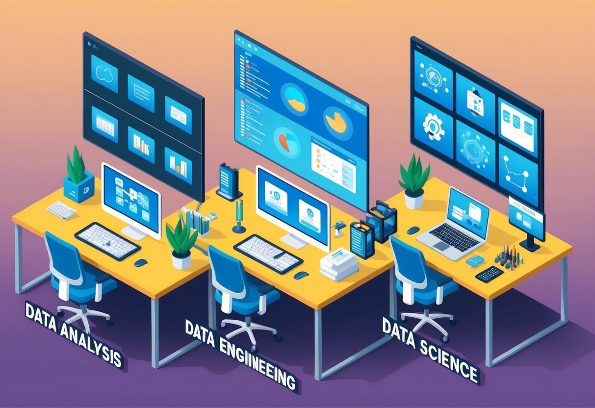
Data analysts, data scientists, and data engineers have specific duties and work with different tools to meet their objectives.
Distinct Responsibilities of Data Professionals
Data Analysts are focused on interpreting data to provide insights. They use tools like Excel, R, or Python to process, clean, and visualize data.
Their reports help businesses understand trends and make decisions.
Data Scientists take this a step further. They apply advanced algorithms, such as machine learning, to predict future trends based on past data.
Their role often requires programming, statistics, and domain expertise.
Data Engineers are essential for building systems that collect, manage, and convert raw data into usable information. They design and implement data pipelines, ensuring data is accessible for analysis.
Their work requires knowledge of data architecture and databases.
Comparing Data Engineers, Analysts, and Scientists
Data Engineers focus on setting up robust infrastructures, while ensuring efficient data flow. Their tasks are more technical, involving complex systems like Hadoop or Spark. This makes them integral in handling large datasets.
Data Analysts are often seen as translators between raw data and business needs. Their role is less technical compared to engineers, concentrating more on making data understandable and actionable for stakeholders.
Data Scientists often bridge the gap between engineering and analysis. They must handle raw data like engineers and derive actionable insights like analysts. This makes their role versatile, as they contribute to both data processing and strategic decision-making.
For more details, view the distinctions in Chartio’s guide on data roles or explore how Caltech differentiates data science and engineering.
Foundations of Data Analysis
Data analysis involves extracting insights from data. Professionals rely on statistical methods, data visualization, and a variety of tools to make informed decisions.
Key components include understanding core principles and harnessing essential tools.
Core Principles of Analyzing Data
Understanding data analysis involves several key principles. It begins with exploratory data analysis (EDA), where analysts gather insights by examining data sets to summarize their main characteristics. This process often makes use of visual methods.
Analysts frequently apply statistical analysis to identify patterns or relationships within the data.
Clear objectives are crucial. Analysts should define their goals before delving into the data, ensuring the chosen methods apply to their questions.
Data quality also plays a critical role, as poor quality can lead to inaccurate insights. Therefore, cleaning and preparing data is a foundational step in any analysis process.
Essential Tools for Data Analysts
Data analysts leverage several tools to perform their tasks effectively.
R and Python are popular programming languages, known for their robust libraries and frameworks for data manipulation and analysis.
SQL is another essential tool, used to query and manage relational databases.
For creating dynamic visualizations, analysts often use Tableau. This software helps transform raw data into understandable formats, aiding the decision-making process.
Additionally, data visualization techniques make it easier to communicate findings to stakeholders.
Building the Data Pipeline
Constructing a data pipeline involves putting together several crucial components that allow for efficient data flow and transformation. It is vital to understand these parts to harness data’s potential effectively.
Key Components of Data Engineering
Data engineers play a significant role in building robust data pipelines. They focus on the architecture that supports data flow through the entire system. This includes designing data infrastructure that can handle different types of data and meet the requirements for big data technologies.
ETL (Extract, Transform, Load) processes are essential in data engineering. They ensure that data is properly extracted from its sources, transformed into useful formats, and loaded into databases or data warehouses. This makes data accessible for analysis and decision-making.
Data engineers also implement data wrangling techniques to clean and organize data, improving the quality and reliability of the final datasets.
Data Collection and Transformation
Data collection is the first step in building a data pipeline. It involves gathering data from various sources such as databases, APIs, or sensors.
Ensuring this process is seamless and secure is crucial for maintaining data integrity.
After collection, data transformation becomes necessary. This involves converting raw data into a structured format that is easier to analyze.
Tools like SQL and Python are often used to modify, cleanse, and enrich data. The goal is to make data ready for further use, whether it’s for reporting, data analysis, or feeding into machine learning models.
Using well-designed data architecture, data pipelines can handle large volumes of data. This ensures scalability and efficiency in handling data tasks.
Keeping up with advancements in big data technologies allows for continuous improvement and adaptation of data pipelines.
Developing Data Science Insights

Data science insights are achieved by using techniques like machine learning and predictive analytics. These methods help in identifying patterns, trends, and making forecasts. Professionals like data scientists play a key role in applying these techniques to turn raw data into actionable outcomes.
Roles of Machine Learning in Data Science
Machine learning is central to data science. It uses algorithms to analyze and learn from data, improving over time without being explicitly programmed.
This capability is crucial for tasks like classification, regression, and clustering.
For instance, in classification, algorithms categorize data into predefined labels, while in regression, they predict continuous values. Clustering groups similar data points to uncover hidden patterns.
Neural networks, a subset of machine learning, are used for more complex tasks, such as image recognition and natural language processing.
Data scientists rely on machine learning because it enables the automation of data analysis, reducing human error and increasing efficiency.
Through machine learning, data can be processed at a scale and speed that would be impossible manually, leading to faster insights and better decision-making.
Creating Predictive Models and Analytics
Predictive models are tools used to forecast future outcomes based on historical data. In data science, these models are essential for predictive analytics.
This involves applying statistical techniques to estimate future trends.
Models like regression are often used here, allowing data scientists to predict future values based on past data.
Neural networks and advanced algorithms further enhance the predictive power by handling large volumes of complex data.
In business, predictive analytics is employed to anticipate customer behavior or demand trends, giving companies a competitive edge.
Data scientists develop these models with precision, ensuring they are robust and reliable for practical use.
Practical Applications of Data Analytics
Data analytics has become crucial for businesses in increasing efficiency and staying competitive. By leveraging data, companies can develop informed strategies and enhance decision-making processes. This section focuses on how data analytics transforms business intelligence and provides tools for maintaining a competitive edge.
Informing Business Intelligence with Data
Data analytics plays a vital role in enhancing business intelligence by converting raw data into actionable insights.
Companies employ data analytics to monitor market trends, customer preferences, and sales performance.
By analyzing these elements, businesses can tailor their strategies to better meet consumer demands.
For example, supermarkets can track purchase patterns to optimize inventory and reduce waste, leading to increased profits and customer satisfaction.
Moreover, data visualization techniques such as charts and dashboards facilitate understanding complex metrics. These tools help decision-makers spot anomalies or opportunities at a glance.
In addition, integrating data analytics with existing business intelligence systems refines forecasting accuracy. This enables firms to anticipate market changes and adjust their operations effectively.
Data-Driven Solutions for Competitive Advantage
Organizations use data to gain a competitive advantage by making data-driven decisions.
By closely examining competitors’ performance and market data, businesses can identify growth areas and potential threats.
A company might innovate products based on unmet needs discovered through thorough data assessment.
In addition to product development, optimizing marketing strategies is another benefit.
Analytics helps companies understand the impact of different campaigns and allocate resources to those that yield the best results.
Furthermore, predictive analytics can highlight future trends, enabling businesses to act proactively rather than reactively.
Using data-driven strategies, businesses strengthen their market position and improve their resilience. This approach empowers them to turn raw data into tangible success.
Managing and Storing Big Data
Managing and storing big data involves using scalable solutions to handle vast amounts of information efficiently. Key areas include setting up data warehouses and choosing appropriate storage solutions like data lakes for large-scale data sets.
Data Warehousing Essentials
Data warehouses play a critical role in organizing and managing big data. These centralized repositories store integrated data from various sources.
By using structured storage, they enable efficient querying and reporting, helping organizations make informed decisions.
Leading technologies include AWS Redshift, Google BigQuery, and Microsoft Azure Synapse Analytics. These platforms provide robust solutions for complex queries and analytics.
Data warehouses are optimized for transactions and offer high-speed performance and scalability.
Their schema-based approach is ideal for historical data analysis and business intelligence. When combined with data lakes, they enhance data management by allowing organizations to store raw and structured data in one place.
Large-Scale Data Storage Solutions
For large-scale data storage, options like data lakes and distributed systems are essential.
A data lake is designed to handle raw data in its native format until needed. It allows the storage of structured, semi-structured, and unstructured data, making it useful for machine learning and analytics.
Apache Hadoop and Apache Spark are popular for processing and managing big data. These frameworks distribute large data sets across clusters, enabling efficient computation.
Services like AWS S3, Azure Data Lake Storage, and Google Cloud Storage are top contenders. They provide scalable and secure storage, ensuring data is readily accessible for analysis and processing.
These platforms support high volume and variety, essential for modern data-driven environments.
Data Engineering and ETL Processes
Data engineering is crucial for managing and organizing vast amounts of data. The ETL process, which stands for Extract, Transform, Load, is a fundamental method used to move data from various sources into a centralized system. This section discusses designing effective data pipelines and improving ETL process efficiency through optimization techniques.
Designing Robust Data Pipelines
A well-designed data pipeline ensures seamless data flow. Data engineers must carefully select tools and technologies to handle large datasets efficiently.
Using tools like Apache Spark can help manage big data due to its fast processing capabilities. Data validation and error handling are critical to maintaining data integrity.
Engineers should implement monitoring solutions to track pipeline performance and identify potential bottlenecks promptly. Keeping scalability in mind allows pipelines to adapt as data volumes increase.
Optimizing ETL for Efficiency
Optimizing ETL processes maximizes data processing speed and reduces resource use.
Engineers can use parallel processing to perform multiple data transformations concurrently, thus speeding up overall data movement.
Leveraging Apache Spark’s distributed computing features allows efficient data handling across clusters.
Incremental data loading minimizes the system’s workload by updating only the modified data.
By refining data transformation scripts and efficiently scheduling ETL jobs, organizations can significantly enhance data processing performance, saving time and resources.
Data Science and Advanced Machine Learning

Data science and advanced machine learning bring together vast data analysis techniques and cutting-edge technology to solve complex problems. Key advancements include deep learning, which emulates human learning, and optimization of machine learning models for improved performance.
Deep Learning and Neural Networks
Deep learning is a subset of machine learning that uses algorithms known as neural networks. It is modeled after the human brain to process data and create patterns for decision-making.
These networks are layered to manage complex data with greater accuracy than traditional models. Popular frameworks like TensorFlow provide tools to build and train deep learning models.
Deep learning is widely used in image and speech recognition, employing large datasets to improve precision.
Neural networks in deep learning help automate tasks that require human-like cognition, such as language translation and autonomous driving. Their structure comprises layers of artificial neurons, allowing them to learn from vast amounts of data through a process known as backpropagation.
This has propelled advancements in fields like natural language processing and computer vision.
Machine Learning Model Optimization
Optimizing machine learning models focuses on enhancing their predictive performance. It involves adjusting algorithms to reduce errors and improve accuracy.
Tools like scikit-learn are essential for performing various optimization techniques, including hyperparameter tuning, which adjusts the algorithm’s parameters to achieve the best results.
Regularization methods help prevent model overfitting by penalizing complex models and ensuring they generalize well to new data.
Cross-validation techniques assess model performance and stability, ensuring they are both accurate and reliable.
By refining these models, data science professionals can derive insightful patterns and projections from complex datasets, contributing to more informed decision-making and innovation in various industries.
The Role of Data Architecture in Technology

Data architecture plays a crucial role in building efficient systems that manage and process data. Key aspects include creating scalable infrastructures and ensuring the security and quality of data.
Designing for Scalable Data Infrastructure
Data architects are responsible for creating systems that handle large amounts of data efficiently. They use various tools and technologies to ensure that data can be easily accessed and processed.
Implementing designs that can grow with business needs is critical. Techniques like cloud computing and distributed databases help in managing resources dynamically.
Efficient data pipelines and storage solutions are essential for supporting big data and analytics. This ensures businesses can make informed decisions based on vast and complex datasets.
Ensuring Data Quality and Security
Maintaining high data quality is vital for any data ecosystem. Data architects design systems that check for inconsistencies and errors.
They use validation rules and automated processes to cleanse data and keep it accurate. Security is another critical focus. Data architecture includes safeguarding sensitive information through encryption and access controls.
Ensuring compliance with data protection laws is essential to prevent breaches. By implementing robust security measures, data architects protect vital information and build trust within the organization.
Programming Languages and Tools in Data Roles

Data roles require proficiency in specific programming languages and tools to handle large datasets and perform complex analyses. These tools and languages are essential for data analysts, engineers, and scientists to effectively manage and interpret data.
Key Languages for Data Analysis and Engineering
Python is widely used for both data analysis and engineering due to its readability and extensive libraries. Libraries like Pandas allow data manipulation and cleaning, which are foundational in data analysis tasks.
SQL is another crucial language, often used for extracting and managing data in databases. For data engineering, knowledge of processing frameworks like Apache Spark can be valuable, as it handles large-scale data efficiently.
R is also popular in data analysis, especially for statistical computing and graphics, offering robust packages for varied analyses.
Using Frameworks and Libraries for Data Science
In data science, combining programming languages with frameworks and libraries creates powerful workflows. Python remains dominant due to its compatibility with machine learning libraries like TensorFlow and Scikit-learn, which simplify model building and deployment.
Apache Hadoop is useful for distributed storage and processing, making it a key tool for managing big data environments. These tools make complex data workflows smoother.
A well-rounded data scientist often uses multiple tools and integrates languages like R and Python, along with others. Leveraging the right tools can significantly enhance data processing capabilities.
Career Paths in Data
Navigating a career in data involves understanding key roles and the potential for growth. These paths range from technical positions to strategic roles in cross-functional teams, each with unique opportunities and compensation trends.
Exploring Opportunities in Data Fields
Data roles have expanded significantly, offering various pathways for professionals. Careers such as data scientist and data engineer play crucial roles in businesses. A data scientist focuses on analyzing data to solve complex problems, while a data engineer designs and maintains systems for data collection and processing.
In addition to these roles, there are positions like AI Innovator and Quantitative Detective that specialize in advanced analytical tasks. Companies in tech, healthcare, finance, and e-commerce actively seek these professionals to drive data-driven solutions. The demand for such skills is rising, and career prospects remain strong.
Understanding Salary and Compensation Trends
Compensation in data careers varies based on role, experience, and industry. Data scientists typically earn competitive salaries due to their specialized skills. According to industry insights, data engineers also enjoy high compensation, reflecting their importance in managing data infrastructure.
Salary can also depend on the industry and location. For instance, positions in tech hubs usually offer higher pay. Career growth in data fields often includes benefits beyond salary, such as bonuses and stock options. Understanding these trends is essential for individuals planning a career in data, allowing them to negotiate effectively and aim for roles that align with their financial goals.
Frequently Asked Questions

Data roles like data analyst, data engineer, and data scientist have their unique functions and require specific skills. Their salaries and responsibilities can vary, as can the interplay of their roles within data-driven projects and teams. Each role plays a critical part in gathering, moving, and analyzing data for real-world applications.
What are the key differences between the roles of data analysts, data engineers, and data scientists?
Data analysts focus on interpreting data and generating insights. They often use statistical tools to communicate findings clearly. Data engineers, meanwhile, handle the architecture of data systems, ensuring data is collected and stored efficiently. Data scientists combine elements of both roles, using algorithms and models to make predictions and extract insights from complex datasets.
How do the salaries for data scientists, data engineers, and data analysts compare?
Data scientists generally have the highest salaries due to their advanced skill set in data modeling and machine learning. Data engineers also earn competitive salaries, given their role in building and maintaining critical data infrastructure. Data analysts, while crucial to data interpretation, usually have slightly lower average salaries compared to the other two roles.
In what ways do the responsibilities of data architects differ from those of data engineers and data scientists?
Data architects design the blueprint for data management systems, ensuring scalability and security. They work closely with data engineers, who implement these plans into functioning systems. Unlike data scientists who analyze and model data, data architects focus on the overall strategy of how data will flow and be stored.
What are the essential skills required for a career in data engineering and data science?
Data engineers need a strong background in programming languages like SQL and Python, and tools for big data processing. Data scientists require a mix of statistical skills, machine learning expertise, and proficiency in programming languages. Both roles benefit from good problem-solving abilities and a solid understanding of data management techniques.
How does the role of data analytics integrate with scientific and engineering projects?
Data analytics helps in assessing trends and patterns within engineering projects, offering insights to improve designs and processes. In scientific projects, analytics aids in experimenting by providing a basis for empirical data analysis. This integration allows teams to make evidence-based decisions and optimize project outcomes.
What are the distinct roles within a modern data team, and what functions do they serve?
A modern data team typically includes distinct roles such as data analysts, data engineers, data scientists, and data architects.
Data analysts interpret and report data findings. Data engineers ensure data systems are operational.
Data scientists apply advanced techniques to derive insights. Data architects structure the data environment, laying out frameworks for other team members to work efficiently.