Weekend Bootcamps

Understanding Linear Regression

Linear regression is a key statistical method used in data science to model the relationship between variables. It helps predict the value of a dependent variable based on one or more independent variables.

Concepts of Linear Regression

Linear regression focuses on establishing a linear relationship between variables. The regression model is expressed as an equation where the dependent variable, often called the response variable, is predicted from independent variables or predictor variables.

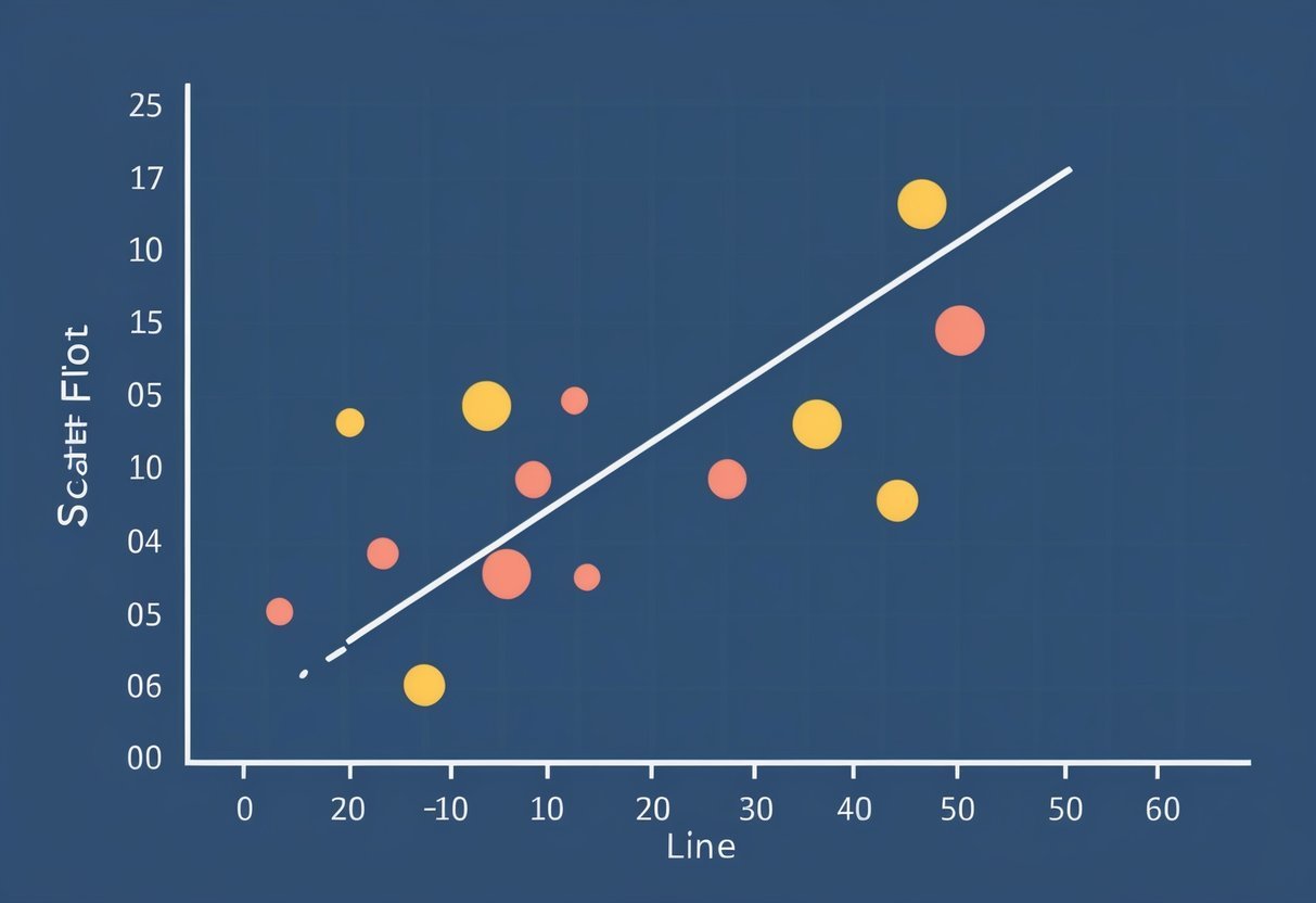
The result is a straight line that best fits the data points, known as the line of best fit.

This method is widely used because of its simplicity and efficiency. The slope of the line indicates the strength and direction of the relationship between the variables. Researchers use this information to make data-driven decisions, like estimating trends over time or understanding how changes in predictors influence the response.

Assumptions of Linear Regression

Linear regression comes with several assumptions that must be satisfied for the model to provide valid results.

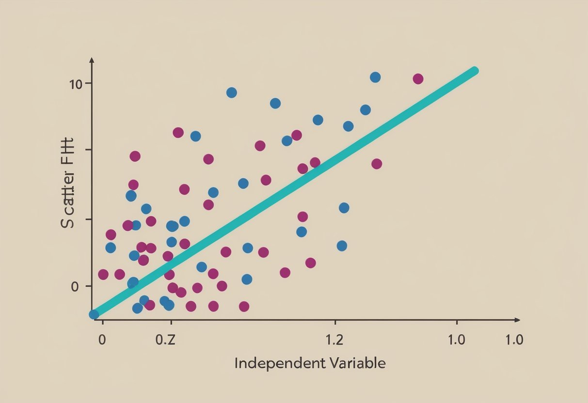
Linearity assumes a straight-line relationship between predictor and response variables. This can be verified through scatter plots or residual plots.

Another assumption is independence, which means observations are not related to each other, ensuring accuracy in predictions.

Homoscedasticity is another important assumption, meaning that the variance of residuals is consistent across all levels of the independent variables. Lastly, the normality of residuals suggests that they should approximately follow a normal distribution.

These assumptions are critical to verify when using linear regression to avoid misleading conclusions.

Diving into Residuals

Residuals play a crucial role in understanding linear regression models. They help reveal how well a model fits the data and highlight any potential issues affecting accuracy. This section explores the definition of residuals and their significance in regression analysis.

Defining Residuals

Residuals are the differences between observed values and predicted values generated by a regression model. When a regression line is drawn through data points, it represents the best-fitted values for that dataset. However, not all data points will lie perfectly on this line.

Residuals are these vertical distances: calculated by subtracting the predicted value from the observed value for each data point.

Residuals provide insight into the level of error in a model. A smaller residual indicates that a predicted value closely matches the observed value, while larger residuals suggest greater inaccuracies.

Residuals can help identify outliers, points that significantly deviate from the expected pattern of the regression line. Such deviations could indicate that other variables might influence the data or that the model needs adjustment.

The Role of Residuals in Regression

Residuals are vital in evaluating the effectiveness of a regression model. They are used in residual analysis, which examines the distribution and pattern of these errors.

A good model will have residuals that are randomly distributed with no discernible pattern. If the residuals display a pattern, it can suggest issues like non-linearity, heteroscedasticity, or model misspecification.

Residual plots, graphical representations of residuals, help assess these aspects visually.

For example, patterns such as a funnel shape in a residual plot may indicate heteroscedasticity, where the variance of errors differs across observations. Consistent residuals can highlight a need for using different techniques or transformations to improve model fit.

Residual analysis aids in enhancing model accuracy and ensuring the reliability of conclusions drawn from regression.

Exploring Residual Plots

Residual plots are essential tools in analyzing linear regression models. They offer valuable insights into the suitability of the model by showing how residual values are distributed and if any patterns exist.

Purpose of Residual Plots

Residual plots serve as a graphical representation of the differences between observed and predicted values in regression models. By plotting residual values against the predicted values or independent variables, one can assess the adequacy of a linear regression model.

Using these plots, one can detect non-linearity, identify heteroscedasticity, and pinpoint influential data points that might affect the model’s accuracy. A plot with a random pattern suggests that the model is appropriate, while visible patterns indicate potential issues.

Interpreting Residual Plots

When interpreting a residual plot, several factors are taken into account. A scatter plot of residuals should appear randomly distributed with no clear patterns for a well-fitting model.

Patterns like a funnel shape could suggest heteroscedasticity, where the variance of errors changes across levels of independent variables.

Symmetry around the horizontal axis is a desirable property. It implies that errors are evenly distributed, confirming the model’s assumptions. Observing clustering or systematic trends might suggest model inadequacies or that important predictor variables are missing.

Checking for these aspects enhances residual plot analysis and ensures the model’s reliability in predicting outcomes.

For more insights on how these characteristics are crucial in regression models, you can explore resources like this comprehensive guide.

Elements of a Residual Plot

Residual plots are essential for assessing linear regression models. They help identify patterns and outliers that might indicate issues with the model. Recognizing these elements is crucial to ensure model accuracy.

Detecting Patterns in Residual Plots

A residual plot shows the residuals on the y-axis and the fitted values on the x-axis. An ideal residual plot displays a random pattern. This randomness suggests that the model is capturing all systematic information, and errors are randomly distributed.

Patterns to watch for:

• Linear patterns: May suggest that a linear relationship is not suitable.
• U-shaped patterns: Can indicate issues like missing variables or incorrect model form.
• High density of points close to the zero line typically indicates a good model fit. Consistency across the horizontal line without forming a clear pattern is key.

A random scatter around the horizontal axis is one of the main characteristics of a good residual plot.

Identifying Outliers and Leverage Points

Outliers appear as points that do not follow the trend of the other points. These points can influence the regression line and skew results.

• Outliers: They can distort the model’s predictions and need careful consideration. Identifying them requires looking for points far from the zero line.
• Leverage points: Unlike typical outliers, these are influential points with high leverage, usually located far from the mass of other data points in terms of x-values. They have the potential to greatly affect the slope of the regression line.

Addressing outliers and leverage points ensures a more reliable model, as these points can lead to biased conclusions if not handled properly.

Statistical Software Tools

Python offers powerful tools for statistical analysis and visualization. Libraries such as Seaborn and Statsmodels stand out by providing robust capabilities for linear regression and residual plot analysis.

Introduction to Python Libraries

Python is widely used in data science due to its extensive collection of libraries for statistical analysis.

Numpy is foundational, offering support for arrays and matrices and many mathematical functions. This support is crucial for handling data sets efficiently.

Another essential library is Matplotlib, which works seamlessly with Numpy for plotting graphs. This makes it easier to visualize complex data relationships and trends.

By leveraging these libraries, users can perform linear regression analysis and create residual plots that illuminate the performance of their data models without diving into overly complex computations.

Utilizing Seaborn and Statsmodels

Seaborn is built on top of Matplotlib, providing a high-level interface for drawing attractive and informative statistical graphics. It simplifies the process of creating residual plots and enhances the visual appeal of data visualizations.

On the other hand, Statsmodels offers a plethora of classes and functions to explore data and estimate statistical models. It also provides built-in functionality for regression analysis, making it easy to assess model assumptions via residual plots.

Using Seaborn and Statsmodels together allows users to effectively analyze and present their regression results, making insights more accessible to non-technical audiences. The combination of these tools offers a comprehensive environment for statistical modeling in Python.

Assessing Model Fit

Assessing model fit is crucial in confirming if a regression model accurately represents the relationship in the data. It involves examining the pattern of residuals and computing specific statistical metrics to ensure precision and reliability.

Analyzing the Residual Distribution

Residuals are the differences between observed and predicted values. A well-fitted model shows a random pattern of residuals scattered around the horizontal axis. If residuals have a funnel shape or curve, this could suggest a poor fit.

Residual plots and scatter plots help visualize these patterns.

Standardized residuals give a clearer picture by adjusting residuals based on their variance. A normal distribution of standardized residuals indicates good model performance.

Correlation and Determination Metrics

R-squared is a key metric in evaluating a regression model. It measures the proportion of variability in the dependent variable explained by the independent variables. A higher R-squared value indicates a better fit, although it does not guarantee prediction accuracy.

MAPE (Mean Absolute Percentage Error) is another important metric. It measures prediction accuracy by calculating the percentage difference between observed and predicted values. This helps in understanding the model’s performance. Reliable models have lower MAPE values.

Distribution of Residuals

In linear regression, checking the distribution of residuals is essential. It helps ensure that the assumptions of the model are met, leading to reliable results. This involves examining normality and testing for homoscedasticity.

Normality in Residuals

Residuals should ideally follow a normal distribution. When residuals are plotted, they should form a symmetric pattern centered around zero.

A normal Q-Q plot provides a graphical method to assess normality.

In this plot, the residual quantiles are compared to the quantiles of a normal distribution. Points lying on or near the line indicate normal residuals. Deviations might suggest that the data does not meet the assumptions of the linear regression, which can affect predictions.

Identifying non-normality allows for adjustments or transformations to improve the model fit.

Testing for Homoscedasticity

Homoscedasticity refers to the residuals having constant variance across different levels of the predictor variables. This means the spread of residuals remains stable, an assumption of linear regression models.

A disturbance in this variance, known as heteroscedasticity, can distort the model’s credibility.

Visual inspection of a residual plot can reveal variance issues. Ideally, the residuals should display a random spread without any clear pattern.

Consistent variance ensures the accuracy and reliability of the model’s predictions. Detecting heteroscedasticity may require transforming variables or employing weighted regression techniques. These adjustments can lead to a more stable relationship between the independent and dependent variables.

Complexities in Linear Models

Understanding the complexities in linear models involves analyzing factors like heteroscedasticity and the independence of error terms. These aspects are crucial for improving the accuracy and reliability of the models.

Heteroscedasticity and its Effects

Heteroscedasticity occurs when the variance of error terms varies across observations.

In a linear regression model, this can lead to inefficient estimates, potentially skewing predictions.

The presence of heteroscedasticity might suggest that the model does not fully capture the data’s complexity.

Identifying heteroscedasticity often involves examining residual plots. A pattern in these plots indicates potential issues.

Correcting heteroscedasticity usually requires transforming the data or using weighted least squares to achieve homoscedasticity, where variances are consistent.

Addressing heteroscedasticity is essential for improving model performance. It helps ensure that predictions are as accurate as possible, allowing the model to generalize well to new data.

Evaluating Independence of Errors

The independence of error terms is another important complexity. It means that the error of one observation should not influence another.

When errors are correlated, it suggests a violation of a key regression assumption, affecting the model’s validity.

Detecting lack of independence can be done using tests like the Durbin-Watson statistic, which helps identify autocorrelation, commonly found in time series data.

Correcting for correlated errors might involve modifying the model structure or using techniques like differencing data points in time series.

Ensuring error independence helps in maintaining the integrity of predictions and enhances the usability of the model.

Advanced Regression Types

Advanced regression models go beyond basic applications, providing deeper insights and more accurate predictions. Two key topics in this area are contrasting multiple linear regression with simple linear regression and understanding their applications in various fields.

Exploring Multiple Linear Regression

Multiple linear regression is a powerful technique that helps in predicting the value of a dependent variable using two or more independent variables.

This model is beneficial in situations where a single predictor isn’t sufficient to explain the variability in the target variable. In the context of machine learning, multiple linear regression is used to uncover relationships in complex data sets.

The process begins with identifying variables that might be relevant, testing their significance, and ensuring the model meets key assumptions like linearity and homoscedasticity.

By evaluating the relationships among multiple variables, this method provides more comprehensive insights compared to simpler models.

Simple vs. Multiple Linear Regression Comparisons

Simple linear regression involves only one independent variable used to predict a dependent variable.

This model is beneficial for understanding the basic influence of a single predictor, but it often lacks the depth required for nuanced analyses. In contrast, multiple linear regression incorporates several predictors, enabling it to address more intricate datasets.

The choice between these methods depends on the research question and the complexity of the data.

When the impact of multiple factors needs to be assessed simultaneously, multiple linear regression becomes essential. Machine learning techniques often prefer multiple predictors for better performance and accuracy in real-world applications.

Case Examples in Regression Analysis

In regression analysis, practical examples from different fields highlight how this statistical method can be applied to understand patterns and make predictions. Applications range from economic forecasting to enhancing sports performance.

Economic Data and Market Trends

Regression analysis plays a key role in analyzing economic data. Economists use it to examine market trends and make predictions about future conditions.

By analyzing historical data, they can identify patterns and factors such as interest rates, unemployment, and inflation. Analysts model these relationships to forecast economic outcomes.

A dataset containing variables like GDP growth and consumer spending can help predict future economic conditions.

This analysis aids in policy-making and business strategy planning. Companies use regression models to predict sales based on various market indicators. These insights enable stakeholders to adjust strategies according to predicted economic shifts effectively.

Sports Performance Analytics

In sports, regression analysis enhances performance evaluation and predictions. For basketball players, statistical models evaluate and predict various performance metrics like scoring, rebounds, and assists.

Data science tools process vast datasets containing game statistics and player attributes. Regression models help teams identify key performance drivers and potential areas of improvement.

For instance, by examining past player performances, teams can predict future player contributions and overall team success.

Using regression, coaches can make informed decisions on player selection and match strategies to optimize performance outcomes. This analytical approach fosters a competitive edge by leveraging data-driven insights into athletic performance.

Practical Applications of Residual Analysis

Residual analysis is vital for enhancing regression models. It’s used in diverse fields to improve predictions and decisions. By examining residuals, professionals can ensure data models accurately reflect real-world dynamics.

Residuals in Business and Finance

In the business and finance sectors, residuals play a crucial role in assessing investment models.

By analyzing residuals, financial analysts can determine the reliability of linear regression models used for forecasting stock prices or market trends. A random distribution of residuals suggests that the model is well-suited to the data, enhancing confidence in financial predictions.

Businesses also use residuals to evaluate customer behavior models. By checking residual patterns, firms can refine marketing strategies and improve customer retention.

For instance, if residuals show patterns, it may indicate that factors influencing sales are not fully accounted for, guiding businesses to adjust their models accordingly.

Healthcare and Residual Plot Utilization

In healthcare, residual plots assist in refining predictive models for patient outcomes.

By analyzing residuals, medical researchers can ensure that the machine learning models used for predicting disease progression are accurate. Patterns in residuals might reveal unaccounted variables such as lifestyle factors in a patient’s health prediction model.

For healthcare management, residual analysis of cost models can identify inefficiencies in hospital operations.

If residuals show a systematic pattern, it might suggest that external factors, like regional healthcare policies, are not fully reflected in the cost predictions. This helps healthcare managers tweak their models for better accuracy and resource allocation.

Frequently Asked Questions

Residual plots are important tools in linear regression analysis, offering insights into model fit and potential problems. They help in determining whether a linear relationship is adequate, what kind of patterns exist, and if the residuals suggest any issues.

How do you interpret a residual plot in linear regression?

In a residual plot, residuals should scatter randomly around the horizontal axis. This pattern suggests a good fit between the model and the data.

If residuals form a pattern, it indicates non-linearity or other issues. A random spread shows that the model’s assumptions hold true.

What indicates a good or bad residual plot?

A good residual plot is one where residuals are evenly distributed around the axis, showing no clear pattern. A bad residual plot shows structured patterns, like curves or clusters, indicating problems like heteroscedasticity or non-linearity.

Can you describe different types of residual plots?

Residual plots can vary. A common type is plotting residuals against predicted values. Another is plotting against each independent variable. Each type helps check different aspects of the model, like variance consistency and linearity. Residual histograms can also show normality of the residual distribution.

How can you identify patterns in residual plots?

Patterns in residual plots, such as curved lines or systematic structures, suggest the model might miss a relationship. Clusters might indicate potential outliers affecting predictions.

These patterns help identify if any assumptions are violated or if transformation of variables is necessary.

What does a residual plot reveal about the fit of a linear model?

Residual plots reveal how well data points fit the linear model by showcasing the residuals’ distribution. Randomly scattered residuals suggest an appropriate fit. Patterns or trends indicate the model might not fit the data well, suggesting a need for revisiting the model.

How do the residuals in linear regression analysis inform model accuracy?

Residuals inform model accuracy by indicating deviations from predicted values.

Smaller and randomly distributed residuals imply higher accuracy and a better model fit.

Large or patterned residuals suggest inaccuracies, indicating the need for further model refinement or alternative approaches.

Understanding Database Design

Database design involves creating a logical structure for storing, organizing, and managing data. A well-designed database ensures efficient data retrieval and modification.

It is crucial for systems that rely on large amounts of information.

A relational database is a type of database that stores data in tables. Each table represents a different kind of entity. Relationships between tables prevent data redundancy and maintain integrity.

Using a DBMS (Database Management System) like MySQL or Oracle helps manage these databases. These systems provide tools for data management, security, and backup. They use SQL (Structured Query Language) to interact with the data.

Key tasks in database design include:

• Data Modeling: Defines how data is connected and stored.
• Normalization: Organizes the data to minimize redundancy.

Learn about normalization step-by-step with this guide on normalization in DBMS.

A well-organized database ensures reliable and quick access to data. Relational databases play a crucial role in applications requiring structured data management.

Essentials of Normalization

Normalization is a crucial aspect of database management. It helps organize data efficiently by reducing redundancy and improving integrity.

What Is Normalization?

Normalization in database design refers to the process of structuring a database into tables and columns. This process follows specific rules that help minimize data redundancy and improve data integrity.

The main forms of normalization include the first, second, and third normal forms. Each of these forms builds upon the previous one, ensuring more efficient data handling.

By organizing tables around specific topics, normalization prevents data anomalies that can occur during data entry, deletion, and updates. This clear and structured approach makes databases easier to manage and maintain.

Importance of Normalization

The importance of normalization lies in its ability to improve database design. By minimizing redundancy, databases become more efficient as they require less storage, reducing potential data anomalies like duplication.

It also enhances data integrity, ensuring that the information remains accurate and consistent across all tables. This makes databases more flexible and adaptable to changing business needs.

Additionally, normalization simplifies data management tasks, supporting easier updates and maintenance.

With these benefits, businesses can ensure their data is reliable and optimized for performance, making normalization a fundamental practice in database design.

Introduction to Normal Forms

In database design, normal forms are used to organize a database efficiently and reduce redundancy. This process ensures that data dependencies are logically stored.

The main forms include First Normal Form, Second Normal Form, and Third Normal Form, each with specific rules and purposes.

First Normal Form (1NF)

First Normal Form focuses on removing duplicate data in a table. It requires that each table cell holds a single value. No column can have multiple values or sets of values. Every row must be unique.

Consider a table of customer orders. To comply with 1NF, avoid storing multiple items in one column. Instead, create separate rows or tables for each item.

This ensures data consistency and simplifies querying. An organized structure eliminates anomalies during data insertion or deletion. 1NF is the foundation for further normalization steps such as Second and Third Normal Form.

Second Normal Form (2NF)

For a table to achieve Second Normal Form, it must first meet the requirements of the First Normal Form. Additionally, all non-primary key attributes should be fully functionally dependent on the primary key.

This means every non-primary key column must relate directly to the entire primary key.

For example, consider a table with a composite key of order ID and product ID. If the customer name depends only on the order ID, a separate table should be created.

This process prevents partial dependency, which simplifies updates and maintains data integrity. Achieving 2NF avoids unnecessary duplication, ensuring efficient database performance.

Third Normal Form (3NF)

Third Normal Form builds upon the principles of the Second Normal Form. It emphasizes the elimination of transitive dependencies.

Every non-prime attribute must depend only on the primary key, and not through another non-prime attribute.

Suppose a table includes fields like employee ID, department ID, and manager name. If the manager name depends on the department ID, which in turn depends on the employee ID, a new table for department details should be created.

Implementing 3NF helps maintain data integrity, reduces redundancy, and avoids update anomalies. Achieving 3NF ensures a robust and efficient database structure.

Advanced Normal Forms

Databases benefit significantly from advanced normal forms, like Boyce-Codd Normal Form and beyond, by reducing anomalies and improving data consistency. These forms tackle complex dependencies and refine structure.

Boyce-Codd Normal Form (BCNF)

Boyce-Codd Normal Form (BCNF) is an upgrade from the Third Normal Form. It is aimed at addressing anomalies due to functional dependencies.

A table is in BCNF if every determinant is a candidate key. This form eliminates redundancy and enforces stricter constraints on functional dependencies.

BCNF is crucial when a table has more than one candidate key and these keys overlap. For instance, in cases where certain attributes depend partially on composite keys, BCNF helps resolve these dependencies.

This results in more reliable data storage by ensuring that non-key attributes are dependent only on superkeys.

BCNF is seen as a critical requirement in database design, thus preventing data anomalies and maintaining consistent integrity across datasets.

Fourth Normal Form (4NF)

Fourth Normal Form (4NF) addresses multi-valued dependencies. Unlike BCNF, which focuses on functional dependencies, 4NF ensures that multiple sets of data are maintained without redundancy across unrelated attributes.

This is significant when dealing with large datasets with multiple independent facts.

A table is in 4NF if it is in BCNF and has no multi-valued dependencies unless trivial.

If a student can enroll in multiple courses and attend various clubs independently, then these attributes should be separated into different tables. This prevents the unnecessary repetition of data and maintains clean and efficient databases.

4NF is crucial when managing complex datasets with repeated groups of facts, allowing for effective storage solutions.

Fifth Normal Form (5NF)

Fifth Normal Form (5NF), or Project-Join Normal Form (PJNF), addresses join dependencies. It ensures that data can be reliably recombined without loss or duplication.

5NF is mostly applied when information is reconstructed through joining.

A table designed with 5NF is free of join anomalies, requiring conditions that decomposition does not hinder data reconstruction.

This is evident where complex relationships exist, like in databases managing multiple vendor contracts, where each contract can be split, yet must be recombinable without mismatch.

5NF is a high level of database normalization that supports the integrity of information when data parts are combined, keeping databases accurate and efficient.

Keys in Database Design

Keys are vital components of database design that ensure data integrity and help define relationships between tables. They play various roles such as identifying records uniquely and linking tables to preserve data consistency.

Primary Keys

A Primary Key uniquely identifies each record in a table. It ensures no duplicate records exist and that each entry is distinct.

Typically, a primary key is a single column, but it can also be a combination of columns. For instance, in a student database, a student ID can be a primary key.

Primary keys are necessary for establishing relationships between tables and maintaining data accuracy. Setting a primary key is essential for data retrieval, manipulation, and storage efficiency.

Foreign Keys

Foreign Keys create a link between two tables, maintaining referential integrity within the database.

A foreign key in one table references the primary key of another table. For example, a foreign key in an orders table might reference the customer ID in a customers table.

This association prevents actions that can damage links between tables, such as deleting a record in a primary key table that a foreign key depends on.

Foreign keys are crucial in structuring relational databases and administering data dependencies.

Candidate Keys

A Candidate Key is a set of attributes that uniquely identify tuples in a table. It can become a primary key, but while each table can have multiple candidate keys, only one can be chosen as the primary key.

Candidate keys should not contain extra attributes—this means removing any redundant attributes.

An example might involve a combination of first name and social security number as potential candidate keys. Not all candidate keys are selected as primary keys, but they provide multiple options for ensuring unique identification within a table.

Composite Keys

Composite Keys are formed by combining two or more columns in a table to uniquely identify a record. They are used when a single column isn’t sufficient to ensure uniqueness across records.

For instance, in an order details table that tracks products sold in different orders, combining order ID and product ID could form a composite key.

This ensures that even if other columns share values, the combination of order ID and product ID remains unique. Composite keys are especially useful in situations where a natural key may not be readily available, offering flexibility in database design.

Functional Dependencies and Anomalies

In database design, functional dependencies help identify relationships between different attributes, contributing to efficient normalization. Meanwhile, data anomalies, such as update, deletion, and insertion errors, can occur without proper dependency management.

Understanding Functional Dependencies

Functional dependencies are key concepts in relational databases, linking columns or sets of columns in a way that dictates relationships. If column A determines column B, then B is functionally dependent on A. This relationship is noted as A → B.

Such dependencies are crucial for eliminating data redundancy. They identify how data should be organized and ensure consistency in database operations.

Recognizing these dependencies helps in designing a database that minimizes redundancy, leading to more efficient storage.

Types of Data Anomalies

Data anomalies occur when expected database behavior differs from actual behavior due to poor design. These anomalies include:

• Update Anomalies: Occur when changes in data require multiple updates, risking inconsistency.
• Deletion Anomalies: Arise when deleting data inadvertently results in losing valuable information.
• Insertion Anomalies: Happen when it’s impossible to add data without including unrelated facts.

These issues highlight the importance of proper normalization, which can be explored further through understanding the five stages of normalization as seen in processes like BCNF.

Proper functional dependencies play a key role in mitigating these anomalies by ensuring accurate and efficient data access.

Designing for Data Integrity

Data integrity is crucial in ensuring that information remains accurate and consistent in a database. Without it, data can become corrupted or misleading.

Data Integrity Types:

1. Entity Integrity: Each table row has a unique identifier (primary key).
2. Referential Integrity: Foreign keys must match primary keys in related tables.

Ensuring Consistency:

Maintaining data consistency means ensuring that data is uniform whenever accessed or modified. This might involve constraints to prevent unauthorized changes that could lead to discrepancies.

A mix of strategies can boost data integrity:

• Normalization reduces redundancy, making databases easier to manage.
• This practice can help enforce data integrity by organizing the database efficiently and minimizing duplication.
• Validation Rules: These ensure only correct data enters the system, reducing errors.

When deciding on normalization levels, it’s important to weigh these benefits against performance needs.

Sometimes, higher normal forms like BCNF are not necessary for every application, depending on specific requirements. Learn more about normalization levels like First Normal Form in this guide.

Security Measures:

Implementing proper access controls also helps maintain data consistency. Limiting who can view or edit information reduces unnecessary changes. Regular audits can also track data changes, ensuring compliance with integrity standards.

In designing databases for data integrity, it’s about striking a balance between ensuring data is correct and maintaining its usefulness and accessibility.

Challenges in Normalization

Normalization is essential for improving database efficiency by reducing redundancy and enhancing data integrity. Despite its benefits, it presents certain challenges that can affect database design and maintenance.

Dealing with Redundancy

Achieving the right balance in database normalization can be tricky.

Over-normalization can lead to increased complexity and may require joining multiple tables to retrieve simple information, impacting performance. This can make the database less flexible and harder to adapt to changing needs.

Storage requirements also play a role when dealing with normalization.

While normalization reduces data redundancy, it can require more disk space due to additional tables and indexes. This can become a concern for large datasets where storage and performance need to be balanced carefully.

Avoiding redundant data is crucial, but it’s equally important to ensure that the database remains flexible and efficient. Properly managing these factors can help maintain a well-functioning database without unnecessary complexity or storage demands.

Normalization Techniques

Understanding normalization techniques is vital in database design to ensure data integrity and efficiency. These techniques eliminate data redundancy and improve data consistency by organizing tables in a structured manner. Below are details on key normalization methods, including steps and complexities involved.

Applying 1NF, 2NF, and 3NF

In First Normal Form (1NF), a table is organized to eliminate repeating groups. Each column should contain atomic values, and each record in the table must be unique. This step simplifies the data structure by ensuring there are no duplicated columns for related data, making it easier to process and manage.

Second Normal Form (2NF) builds upon 1NF by removing partial dependencies.

A table reaches 2NF when all non-key attributes are fully functional dependent on the entire primary key. In simpler terms, this means eliminating dependencies on a part of a composite primary key, thereby ensuring that partial relationships are addressed.

Third Normal Form (3NF) addresses transitive dependencies.

A table is in 3NF when non-key attributes are not dependent on other non-key attributes. By resolving transitive dependencies, data is grouped more logically, enhancing data integrity. Implementing 3NF typically involves creating new tables to isolate critical dependencies.

Beyond 3NF: Advanced Normalization

After achieving 3NF, advanced techniques handle more complex dependencies.

Boyce-Codd Normal Form (BCNF) is a stronger version of 3NF and aims to address cases where multiple overlapping candidate keys exist. In BCNF, every determinant must be a candidate key, ensuring a higher level of structure.

Fourth Normal Form (4NF) focuses on removing multi-valued dependencies. This normal form requires that a table not contain more than one independent multi-valued dependency on a single table. Splitting tables further into related sub-tables helps achieve 4NF and reduces potential redundancies.

Fifth Normal Form (5NF) deals with join dependencies, ensuring tables are structured so that they can be reconstructed from smaller, related tables without loss of information. Achieving 5NF often involves understanding complex relationships and ensuring minimal data redundancy while preserving necessary connections between tables.

SQL and Normalization

Normalization in SQL is a vital process in database design that aims to reduce redundancy and improve data integrity. By organizing data into tables and defining relationships, normalization ensures efficient storage and easy retrieval of information. This process involves dividing larger tables into smaller ones and structuring them to minimize duplication.

SQL queries benefit from normalization as they operate on efficiently organized databases. By following rules called normal forms, usually listed as 1NF through 5NF, databases become more consistent and dependable. Database normalization reduces data anomalies, such as insertion, update, and deletion issues.

First Normal Form (1NF) requires eliminating duplicate columns from the same table and ensuring each column contains atomic values.

Second Normal Form (2NF) builds on this by ensuring all non-key attributes are fully functionally dependent on the primary key.

Third Normal Form (3NF) further removes columns not connected to the primary key. It simplifies SQL queries by reducing complexity and unnecessary joins. Advanced forms like Boyce-Codd Normal Form (BCNF) and Fourth Normal Form (4NF) ensure even higher levels of data integrity.

The benefits of normalization include structured data organization and elimination of redundancy. Databases become more scalable and easier to maintain. SQL queries run more efficiently, providing faster results and enhanced performance.

Effective application of normalization principles contributes to the robustness and readability of SQL queries, making them powerful tools in data manipulation and analysis. As a best practice, applying normalization in SQL design is essential for creating high-quality databases.

Denormalization for Performance

Denormalization involves adding redundancy to a database to improve query performance. By storing duplicate copies of data, it reduces the need for complex joins between tables. This approach can speed up data retrieval, especially in large databases where frequent queries occur.

Benefits of Denormalization:

• Improved Read Performance: Queries can access data from fewer tables, making data retrieval faster.
• Simplified Queries: Reduces the need for complex joins, making queries simpler and easier to manage.

While denormalization has benefits, it also comes with trade-offs. Data redundancy can lead to inconsistencies if not managed carefully.

When designing a database, it’s essential to find a balance between normalization’s structure and denormalization’s speed.

In many systems, hybrid approaches are used, where some parts of the database are normalized, and others are denormalized. This mix allows databases to maintain data integrity while optimizing for performance where necessary.

In essence, the choice depends on the specific needs and constraints of the database design.

Choosing denormalization should be guided by the system’s workload and the types of queries it will process.

Applications with heavy read operations may greatly benefit from this approach. However, it is crucial to continuously monitor and adjust based on the database’s evolving requirements.

Frequently Asked Questions

Normalization is crucial for reducing redundancy and ensuring efficiency in databases. It involves various stages and forms that improve data design, integrity, and performance.

What are the stages and benefits of normalizing a database?

Normalization involves several stages, often categorized as normal forms. These stages help in organizing data efficiently by minimizing duplicate information. The benefits include improved data integrity and reduced storage space, leading to better database management.

How do the different forms of normalization improve database design?

Different forms, such as 1NF, 2NF, and 3NF, aim to systematically reduce redundancy. Each stage targets specific issues. For instance, 1NF eliminates duplicate records, while 2NF and 3NF address more complex redundancies and dependencies, enhancing the overall design and structure.

What are examples of 1NF, 2NF, and 3NF in database normalization?

1NF, or the First Normal Form, involves removing repeating groups and ensuring atomic columns. 2NF, the Second Normal Form, eliminates partial dependencies. 3NF, the Third Normal Form, focuses on removing transitive dependencies, further streamlining data representation and reducing unnecessary data duplication.

How does normalization affect performance and integrity in a database system?

Normalization enhances data integrity by ensuring consistency and reducing anomalies. While it can make querying more complex, the trade-off often results in improved data accuracy. As redundant data is minimized, storage efficiency is enhanced, positively affecting performance.

What is the role of functional dependencies in database normalization?

Functional dependencies guide the normalization process by defining relationships between attributes. They help determine how data is logically stored within tables. Recognizing these dependencies is essential for fulfilling the requirements of various normal forms, ensuring data is efficiently organized and maintained.

Can a database be over-normalized, and if so, what are the implications?

Yes, a database can be over-normalized, leading to complexities in data retrieval. When a database is overly broken down into small tables, it can result in increased join operations, which may slow down data retrieval processes. It’s crucial to balance normalization to maintain both structure and performance.

Understanding Logistic Regression

Logistic regression is a powerful tool in machine learning, used primarily for classification tasks. It leverages the logistic function to estimate probabilities and allows classification into distinct categories.

This section explores its essentials, comparing it to linear regression, and discusses different types like binary and multinomial logistic regression.

Logistic Regression Essentials

Logistic regression is a method used in machine learning for classification tasks. While linear regression predicts continuous outcomes, logistic regression deals with probability estimation. For instance, it determines the probability that a given instance falls into a specific category. The key mathematical element here is the logistic function. It outputs values between 0 and 1, which can be interpreted as probabilities.

This technique is particularly useful in binary classification, where there are two outcomes, like “yes” or “no.” A logistic regression model uses these probabilities to make decisions about class membership. For instance, it might predict whether an email is spam or not. This approach can be extended to more complex scenarios, such as multinomial and ordinal logistic regression, where there are more than two categories.

Comparing Logistic and Linear Regression

While both logistic and linear regression are predictive models, they serve different purposes. Linear regression predicts continuous data, finding the best-fit line through data points, while logistic regression handles classification tasks, predicting categorical outcomes using probabilities. The goal of logistic regression is to find a function that assesses the likelihood of the outcome being a particular class.

In a linear regression model, errors are measured in terms of the distance from the line of best fit. In a logistic regression model, the likelihood of correctness based on the logistic function is the measure. This difference in target outcomes makes logistic regression more suited for tasks where the end goal is to classify data into categories rather than predict numerical values.

Types of Logistic Regression

Logistic regression can take various forms to handle different classification scenarios. Binary classification is the simplest form, addressing problems with two possible outcomes. For more complex cases, such as classifying multiple categories, multinomial logistic regression is applied. It allows a comprehensive probability estimation across several categories instead of just two.

Another type is ordinal logistic regression, which deals with ordered categories. It is handy when dealing with ranked data, such as levels of satisfaction from surveys. This type helps maintain the order among choices, providing a significant advantage when the hierarchy in the outcome categories matters. These variations enable logistic regression to adapt to a broad range of classification problems.

Building Blocks of Logistic Regression

Logistic regression is a fundamental technique in machine learning, often used for binary classification. This method relies heavily on the sigmoid function, coefficients, and an intercept to map inputs to predicted outcomes, which are interpreted as probabilities. Understanding these elements is crucial for grasping how logistic regression works.

Understanding the Sigmoid Function

The sigmoid function is a mathematical tool that transforms input values, mapping them to outputs between 0 and 1. This transformation is essential for logistic regression as it converts linear predictions into probabilities. The formula used is:

[ text{Sigmoid}(z) = frac{1}{1 + e^{-z}} ]

where ( z ) represents a linear combination of input features. The sigmoid curve is S-shaped, smoothly transitioning probabilities as input values change. It ensures predictions can easily be interpreted as probabilities, with values near 0 or 1 indicating strong class membership.

The Role of Coefficients and Intercept

Coefficients in logistic regression represent the importance of each feature in predicting the outcome. These are weights assigned to each input variable, determining their influence on the model’s predictions. The model also includes an intercept, a constant term that shifts the decision boundary.

Together, coefficients and the intercept form a linear equation:

[ z = b_0 + b_1x_1 + b_2x_2 + ldots + b_nx_n ]

where ( b_0 ) is the intercept, and ( b_1, b_2, ldots, b_n ) are the coefficients for each feature ( x_1, x_2, ldots, x_n ). Adjusting these values during model training helps in fitting the model to the data.

Interpreting Log-Odds and Odds

Logistic regression outputs are often expressed in terms of log-odds, which reflect the natural logarithm of the odds of an outcome. The odds represent the ratio of the probability of the event to the probability of non-event. The logit function converts probabilities into log-odds:

[ text{Logit}(p) = log left(frac{p}{1-p}right) ]

Understanding log-odds helps in interpreting the output in a linear manner, making it easier to assess how each variable influences the likelihood of an event. Odds greater than 1 suggest a higher likelihood of the event occurring, providing insights into feature impact.

Machine Learning Foundations

Understanding the basics of machine learning is essential for grasping its complexities. Here, the focus is on the differences between supervised and unsupervised learning, preparing data, and key concepts in machine learning.

Supervised vs. Unsupervised Learning

Supervised learning uses labeled datasets to train algorithms, ensuring the model can predict outputs with correct input data. Common in classification algorithms, it develops models that learn from data with known answers. This includes applications like spam detection and image recognition.

Unsupervised learning, on the other hand, works with unlabeled data. It identifies patterns and structures without explicit instructions, commonly used in clustering and association tasks. These methods are useful for exploratory data analysis, discovering hidden patterns or groups in data.

Data Preparation and Feature Engineering

Data preparation involves cleaning and organizing a dataset to ensure it is accurate and complete. Missing values are handled, and outliers are addressed to improve model performance.

Feature engineering is the process of transforming raw data into meaningful features that enhance the predictive power of machine learning algorithms.

This step is crucial for distinguishing independent variables, which provide essential insights for models. Engineers may encode categorical variables or normalize data to ensure all features contribute effectively.

Proper data preparation and feature engineering can significantly boost the accuracy of predictive modeling.

Key Concepts in Machine Learning

Several key concepts underpin machine learning, including the learning rate, which affects how quickly a model learns. Choosing the right learning rate is vital for efficient training. If set too high, the model may overshoot optimal solutions; if too low, it may learn too slowly.

Understanding the dataset and selecting appropriate machine learning algorithms are critical. Algorithms like logistic regression are popular choices for classification tasks, where predicting categorical outcomes is necessary. Proper training data is essential for building models that generalize well to new data and perform accurately on unseen examples.

Mathematical Framework

The mathematical framework of logistic regression involves key concepts and techniques. These include probability and prediction, maximum likelihood estimation, and the logistic function. Each aspect is crucial to understanding how logistic regression operates as a statistical method to classify data based on a dependent variable’s predicted probability.

Probability and Prediction

In logistic regression, probability and prediction work hand in hand to classify outcomes. The model determines the predicted probability that a given input falls into a specific category. Unlike linear regression, which predicts continuous output values, logistic regression predicts categorical outcomes, typically binary.

The model uses a sigmoid function to map predictions to a range between 0 and 1, representing probabilities. For example, if predicting whether a student will pass or fail an exam, the output value indicates the probability of passing. A cutoff, often 0.5, determines classification: above the threshold predicts one category, while below predicts another.

Maximum Likelihood Estimation

Maximum likelihood estimation (MLE) is a statistical method crucial in logistic regression for parameter estimation. The goal is to find parameters that maximize the likelihood function, reflecting how probable the observed data is given model parameters.

Iterative optimization algorithms, such as gradient descent, are often used to adjust parameters, seeking to maximize the log-likelihood because of its computational efficiency. This adjustment improves the model’s accuracy in predicting categorical outcomes by ensuring the estimated probabilities align closely with observed data. MLE helps refine the model’s coefficients, enhancing prediction reliability.

Understanding the Logistic Function

The logistic function is central to logistic regression, converting a linear combination of inputs into a probability. It maps input values to a range between 0 and 1, making it suitable for classification tasks. The function, also known as a sigmoid curve, is defined as:

[
P(y=1|X) = frac{1}{1 + e^{-(beta_0 + beta_1X)}}
]

Here, ( beta_0 ) and ( beta_1 ) are coefficients, and ( e ) is the base of the natural logarithm. This function’s S-shape ensures that extreme input values still produce valid probabilities. By understanding how this function operates, one can appreciate logistic regression’s capability to model complex relationships in classification tasks.

Model Training Process

The training process of logistic regression involves optimizing model parameters using gradient descent. Key factors include minimizing the cost function to achieve an effective model and using regularization to prevent overfitting. These elements work together to enhance the performance and predictive power of the logistic regression model.

Utilizing Gradient Descent

Gradient descent is crucial for training a logistic regression model. This optimization algorithm iteratively adjusts model parameters to minimize errors in predictions. It uses the gradient, or slope, of the cost function to decide how much to change the parameters in each step.

By moving in the opposite direction of the gradient, the algorithm reduces the cost and brings the model closer to the optimal state.

Choosing a suitable learning rate is vital. A high learning rate might cause the model to miss the optimal solution, while a low rate can slow down the process.

Different types of gradient descent, like batch, stochastic, and mini-batch, offer variations that influence efficiency and convergence speed.

Cost Function and Model Optimization

The cost function in logistic regression is often log loss, which measures how well the model predicts the training data. It calculates the difference between predicted probabilities and actual class labels, aiming to minimize this value. The smaller the log loss, the better the model predicts outcomes.

Model optimization involves solving this optimization problem by finding the parameter values that minimize the cost function.

Using methods like gradient descent, the algorithm repeatedly updates parameters to find the best-fit line or decision boundary for data classification. Effective model optimization ensures the logistic regression algorithm performs accurately.

Handling Overfitting with Regularization

Overfitting occurs when a logistic regression model learns noise in the training data, leading to poor generalization to new data.

Regularization techniques help manage this by adding a penalty term to the cost function. This term discourages overly complex models by keeping the parameter values smaller.

Two common types of regularization are L1 (Lasso) and L2 (Ridge). L1 regularization can shrink some coefficients to zero, effectively selecting features. Meanwhile, L2 regularization distributes the penalty across all coefficients, reducing their magnitude without setting them to zero. Both methods help in maintaining a balance between fitting the training data and achieving generalization.

Accuracy and Performance Metrics

Accuracy is a fundamental metric in classification problems. It reflects the percentage of correct predictions made by the model over total predictions. However, accuracy alone can be misleading, especially in datasets with class imbalance.

For example, if 90% of the data belongs to one class, a model that always predicts that class will have 90% accuracy.

To overcome this limitation, precision, recall, and F1 score are also used. These metrics provide a clearer picture of model performance.

Precision measures the accuracy of positive predictions, while recall, also known as sensitivity, measures the model’s ability to capture all positive instances. The F1 score combines precision and recall into a single value, making it useful when dealing with uneven classes.

Applying the Threshold Value

The threshold value in logistic regression determines the point at which the model classifies an instance as positive. This threshold impacts sensitivity and specificity.

Setting a low threshold can lead to more positive predictions, increasing recall but possibly decreasing precision. Conversely, a high threshold might improve precision but reduce recall.

A common approach involves using cross-entropy to estimate the optimal threshold.

Cross-entropy measures the difference between true values and predicted probabilities, providing insight into finding the best balance between precision and recall. This balancing act is critical in predictive modeling, where both false positives and false negatives have different costs.

ROC Curve and AUC

The ROC curve is a graphical representation that illustrates the performance of a classification model at various threshold values. It plots the true positive rate against the false positive rate.

The goal is to have the curve as close to the top-left corner as possible, indicating high sensitivity and specificity.

A key component is the Area Under the Curve (AUC), which summarizes the ROC curve into a single value.

An AUC near 1 suggests excellent model performance, while an AUC near 0.5 indicates a model with no predictive ability. Evaluating the AUC helps in comparing different models or assessing the same model under various conditions.

Real-World Applications of Logistic Regression

Logistic regression is a crucial tool in various fields due to its effectiveness in predicting binary outcomes and tackling classification problems. It is widely applied in healthcare, especially for cancer diagnosis, and aids in business decision making.

Predicting Binary Outcomes

Logistic regression excels in predicting binary outcomes, such as yes/no or success/failure decisions. It models the probability of a certain class or event existing, which makes it suitable for tasks involving classification problems.

The algorithm uses a logistic function to compress output values between 0 and 1, enabling clear distinctions between the two possible categories.

In fields like marketing, logistic regression helps in predicting the likelihood of a customer purchasing a product based on various attributes. This ability to predict can guide companies in making informed strategic decisions.

Application in Healthcare: Cancer Diagnosis

In healthcare, logistic regression is often used for cancer diagnosis. Its role involves discerning whether a condition like gastric cancer is present, based on real-world clinical data.

By analyzing various predictors, such as patient history and test results, logistic regression models help estimate the probability of cancer.

This data-driven approach allows healthcare professionals to prioritize patient care effectively and facilitates early detection strategies. Such applications are crucial in improving treatment outcomes and resource management in medical settings.

Business Decision Making

Within the business realm, logistic regression informs decision making by handling classification tasks like credit scoring and customer churn prediction.

By classifying potential defaulters, financial institutions can mitigate risks. The model predicts whether a customer will default, using historical data to assign probabilities to different outcomes.

In retail, logistic regression analyzes customer attributes to predict behavior, aiding in retention strategies.

Companies can focus on customers likely to leave, implementing targeted interventions to reduce churn, thus optimizing customer relationship management strategies. This capability empowers businesses to act proactively, enhancing competitive advantage.

Using Logistic Regression with Python

Logistic regression is a popular method for classification tasks in machine learning. This section focuses on implementing logistic regression using Python’s scikit-learn library. It covers the basics of scikit-learn, coding the logistic regression model, and interpreting the results.

Introduction to Scikit-Learn

Scikit-learn is a powerful Python library used for data mining and machine learning. It is user-friendly and supports various algorithms, including classification methods like logistic regression.

One key feature is its ability to handle large datasets efficiently.

With scikit-learn, users can easily split datasets into training and testing sets, apply different models, and evaluate their performance. Scikit-learn’s consistency in syntax across functions and models makes it accessible for beginners and experts alike.

Coding Logistic Regression with sklearn.linear_model

To start coding a logistic regression model, the sklearn.linear_model module provides a straightforward implementation. Begin by importing the module and loading your dataset. Preprocessing the data, such as scaling, often improves model performance.

from sklearn.linear_model import LogisticRegression
from sklearn.model_selection import train_test_split

# Example dataset split
X_train, X_test, y_train, y_test = train_test_split(X, y, test_size=0.2, random_state=42)

# Initialize and train the model
model = LogisticRegression()
model.fit(X_train, y_train)

Regularization can be applied to prevent overfitting. Options such as L1 or L2 regularization are available by setting the penalty parameter. The model then generates predictions based on the test data.

Interpreting Model Output

Interpreting logistic regression output involves analyzing various metrics. Accuracy, precision, recall, and the confusion matrix are frequently used to assess model performance. These metrics offer insights into how well the predictions align with the actual classes.

The coefficients of the logistic regression model indicate the strength and direction of the relationship between input features and the target variable. An understanding of these coefficients can be critical for making informed decisions based on the model’s insights.

Visualizations, such as ROC curves, can help further evaluate the model’s ability to distinguish between classes.

These plots provide a graphical representation of the trade-off between sensitivity and specificity, aiding in fine-tuning the model for optimal results.

Key Considerations

Careful planning is necessary when using logistic regression for classification. Important factors include the quality and size of the dataset, handling multicollinearity, and understanding the assumptions and limitations inherent in logistic regression models.

Sample Size and Data Quality

To achieve accurate results, a large enough sample size is crucial for logistic regression. When the sample size is too small, the model may not capture the variability in data effectively. This can lead to inaccurate predictions.

Large datasets with diverse data points provide the stability and reliability needed in a model.

Data quality also plays a vital role. The presence of noise and missing data can skew results.

It’s essential to clean the data before modeling. Ensuring the variables are representative and relevant to the problem will help improve model performance. Moreover, each observation should be independent of others to avoid biased results.

Addressing Multicollinearity

Multicollinearity occurs when independent variables are highly correlated. This can cause issues in logistic regression as it may lead to unreliable estimates of coefficients.

It becomes challenging to determine the individual effect of correlated predictors, which can lead to misleading conclusions.

One way to address multicollinearity is through techniques like removing or combining correlated variables. Using Principal Component Analysis (PCA) can also help by transforming the original variables into a new set of uncorrelated variables.

Detecting and managing multicollinearity is crucial for model accuracy and interpretability.

Assumptions and Limitations

Logistic regression assumes a linear relationship between the independent variables and the log odds of the outcome. When this assumption is not met, predictions may not be accurate.

The model also assumes a binomial distribution of the data, which is important for valid results.

Another assumption is the absence of multicollinearity, which, if violated, can cause unreliable coefficient estimates.

While logistic regression is efficient for binary outcomes, it might not capture complex patterns like some advanced models. Understanding these limitations helps in setting realistic expectations about model performance.

Model Implementation

Implementing logistic regression models involves careful integration into existing systems and following best practices for deployment. This ensures the models are efficient, reliable, and easy to maintain.

Integrating Logistic Regression into Systems

Integrating a logistic regression model involves several key steps. First, it’s essential to prepare the dataset by ensuring it is clean and structured. In Python, this process often includes using libraries like Pandas and NumPy for data manipulation.

Properly setting the random_state during model training ensures reproducibility, which is crucial for consistent results.

Code implementation usually follows, where the model is defined and trained. The epochs parameter is particularly important when training iterative models, although it is not directly applicable to logistic regression as it is for neural networks.

The model’s parameters are then fine-tuned to improve performance.

Logistic regression models can be integrated into a system by exporting them with tools like Pickle or Joblib for easy deployment and future access. Ensuring compatibility with the system’s other components is key to a smooth integration.

Model Deployment Best Practices

Deploying a logistic regression model requires careful consideration of several factors to ensure it performs well in a live environment.

It’s essential to monitor performance metrics consistently. This includes tracking the model’s accuracy and adjusting parameters as necessary based on real-world data.

Model deployment should be supported by automation tools to streamline processes such as data updates and retraining schedules.

Using continuous integration and delivery (CI/CD) pipelines can enhance reliability and scalability.

Integrating these pipelines can automate much of the model update process, making them less error-prone and reducing the need for manual intervention.

Implementing these best practices ensures that logistic regression models remain efficient, providing reliable predictions and insights in production systems.

Advancements and Future Directions

Machine learning continues to evolve rapidly, especially in the area of classification tasks such as logistic regression. The ongoing development in this field is characterized by emerging trends and an expanding ecosystem that enhances algorithm efficiency and application.

Emerging Trends in Classification Algorithms

Recent advancements in classification algorithms are transforming machine learning. One significant trend is the integration of deep learning techniques, which improve model accuracy and adaptability. These enhancements are crucial for complex tasks like image and speech recognition.

There is also a growing focus on model interpretability. This shift aims to make algorithms, like logistic regression, more transparent, helping users understand decision-making processes.

These trends are pushing the boundaries of what classification algorithms can achieve, making them more reliable and user-friendly.

Evolving Machine Learning Ecosystem

The machine learning ecosystem is expanding, driven by advancements in hardware and software tools. New frameworks make the development of classification algorithms more accessible and efficient.

Libraries such as TensorFlow and PyTorch provide robust support for implementing logistic regression and other models.

Additionally, cloud-based platforms enhance scalability and efficiency. They allow for processing large datasets necessary for training sophisticated classification models.

This evolving ecosystem supports researchers and developers by providing tools to build more accurate and efficient machine learning algorithms, positioning the field for continued innovation.

Frequently Asked Questions

Logistic regression is a popular tool for classification tasks in machine learning, offering both simplicity and effectiveness. It can be implemented using programming languages like Python and serves well in a variety of classification scenarios, from binary to multi-class problems.

How can logistic regression be implemented for classification in Python?

Logistic regression can be implemented in Python using libraries such as scikit-learn. One needs to import LogisticRegression, fit the model to the training data, and then use it to predict outcomes on new data.

What is an example of logistic regression applied to a classification problem?

An example of logistic regression is its use in predicting credit approval status. By modeling the probability of loan approval as a function of applicant features, logistic regression can distinguish between approved and denied applications based on previous data patterns.

What are the assumptions that must be met when using logistic regression for classification?

Logistic regression assumes a linear relationship between the independent variables and the log odds of the dependent variable. It also requires that observations are independent and that there is minimal multicollinearity among predictors.

How can I interpret the coefficients of a logistic regression model in the context of classification?

Coefficients in logistic regression represent the change in the log odds of the outcome for each unit change in a predictor. Positive coefficients increase the probability of the class being predicted, while negative ones decrease it.

How does logistic regression differ when dealing with binary classification versus multi-class classification?

In binary classification, logistic regression predicts one of two possible outcomes. For multi-class classification, methods like one-vs-rest or softmax regression are used to extend logistic regression to handle more than two classes.

Why is logistic regression considered a linear model, and how does it predict categorical outcomes?

Logistic regression is considered linear because it predicts outcomes using a linear combination of input features. It predicts categorical outcomes by mapping predicted probabilities to class labels. The probabilities are derived using the logistic function.

Understanding Matplotlib and Figures

Matplotlib is a powerful Python library for creating intricate and robust plots and graphs. Central to its structure are figure objects, which serve as the foundational canvas for all plotting activities involving various elements like axes and artists.

What Is Matplotlib?

Matplotlib is a widely-used plotting library in Python that enables users to produce 2D and 3D graphs. It is especially valued for its versatility, capable of generating plots ranging from simple line charts to complex visualizations.

This library is essential for developers and analysts who need to visualize data efficiently. Its functionality can extend through various interfaces, such as pyplot, which simplifies creating and managing graphs.

Matplotlib supports different backends for rendering, allowing integration with GUI toolkits like Tkinter and Qt. It is also versatile with graphics formats such as PNG, PDF, and SVG. This flexibility makes it a preferred choice for professionals seeking to include visual data interpretations in applications or reports.

Overview of Figure Objects

In Matplotlib, a figure object acts as a drawing canvas on which everything else is plotted. These objects contain all plot elements, including one or more axes, which are essential for plotting data.

The figure can be customized with different sizes, background colors, and resolutions to fit specific visualization needs.

Creating a figure in Matplotlib can be done via functions like plt.figure() or plt.subplots(), which set up the base for further customization and plotting.

Figures are integral to managing multiple subplots and ensuring that each graph element is appropriately arranged and displayed. This structure aids developers and analysts in organizing complex sets of data into comprehensible visuals.

Setting Up the Environment

Setting up Matplotlib involves installing the library correctly and knowing the essential imports needed to work efficiently with its features. This helps in creating plots and graphs in Python, especially when using interactive environments like Jupyter Notebook.

Installing Matplotlib

To begin using Matplotlib, it needs to be installed in the Python environment. Users can install it using pip, the package manager for Python. They can open the terminal or command prompt and type the following command:

pip install matplotlib

For those using Jupyter Notebook, installing Matplotlib within the notebook itself is possible by using magic commands. Adding ! before the command allows running shell commands directly in Jupyter cells:

!pip install matplotlib

Users on macOS might need additional software, such as libpng and Freetype, which can be installed using Homebrew.

It’s crucial to ensure that Python and Jupyter Notebook are also properly configured as they are often used together.

Essential Import Statements

Once Matplotlib is installed, importing the necessary components is the next step.

The most common import involves pyplot, a module within Matplotlib that provides a MATLAB-like interface. Here is how it is typically done:

import matplotlib.pyplot as plt

The alias plt is widely used in examples and tutorials, making the code easier to understand.

In Jupyter, magic commands like %matplotlib inline are often used. These commands enable plots to appear directly in the notebook upon execution.

Additionally, users may import other modules or functions from Matplotlib depending on their specific needs, like working with interactive plots or configuring plot styles. Having the correct imports ensures a smooth and efficient plotting experience.

Creating Figures in Matplotlib

Creating figures in Matplotlib is essential for visualizing data. A figure represents the entire drawing area, capable of containing multiple plots. This section discusses the Figure class, the plt.subplots() function, and how to customize figure size and resolution.

The Figure Class

The Figure class in Matplotlib is the foundation for all graphics. It serves as a container that holds all plot-related elements.

This class is accessed using the pyplot interface, which simplifies creating figures by managing backend operations and window interfaces. You can create a figure by calling pyplot.figure(), which returns a Figure object to which you can add plots.

The interface allows for setting parameters such as size and resolution. Understanding the role of Figure class helps in organizing and managing complex visualizations involving multiple plots or graphs within a single or several figures.

Utilizing the plt.subplots() Function

The plt.subplots() function is a versatile tool for creating figures with multiple plots, also known as subplots. It simplifies the process of arranging them within a grid layout.

By specifying the number of rows and columns, plt.subplots() returns a Figure object and an array of Axes objects for plotting data.

This function is helpful when analyzing datasets with multiple variables. It enables visualization within the same figure, making comparisons easier.

Additionally, plt.subplots() provides a convenient approach to customizing how each subplot is positioned and sized within the overall figure.

Customizing Figure Size and DPI

Figure size and resolution are crucial for the clarity and readability of plots.

Using the figsize and dpi parameters, you can adjust the physical dimensions and resolution of a figure created with pyplot.figure() or plt.subplots(). The figsize parameter takes a tuple representing width and height in inches, while dpi sets dots per inch for the figure’s resolution.

Customizing these settings helps ensure that plots look good across different devices and formats. This flexibility allows for tailoring visualizations to suit presentations, web displays, or print publications, making your data easier to interpret visually.

Axes and Subplots

Axes and subplots are essential components when creating visualizations with Matplotlib. These elements allow precise control over how data is presented, enabling flexible arrangements and detailed customizations.

Adding Axes to a Figure

Adding axes to a figure in Matplotlib can be done in several ways. The most common method is using add_subplot, which places a subplot at specified grid positions within the figure. This approach is handy for quickly sketching out multiple plots.

Alternatively, add_axes offers more control, allowing users to specify the exact position and size of axes using a list of coordinates. This is useful for custom layouts.

Understanding the distinction between these methods helps in designing clear and organized visualizations. For more detailed instructions on positioning, refer to the Introduction to Axes.

Configuring Subplots

Configuring subplots involves arranging multiple axes within a single figure. The pyplot.subplots function simplifies this by providing a grid layout with shared properties like x-axis or y-axis labels.

Users can also customize the arrangement to display different types of plots side by side or in a grid. Adjusting the tight_layout or using GridSpec enhances readability by optimizing space around each subplot.

These tools make it easier to compare plots or display different datasets within the same figure, as described in the Arranging Axes in a Figure.

Understanding Axes Object vs Axis

The axes object and axis are related yet distinct in plotting with Matplotlib. The axes object is a part of the figure that contains the plot. It controls the display of elements like ticks, labels, and grids.

On the other hand, the axis refers specifically to one of the reference lines, either x or y.

This distinction is crucial in customizing chart elements, where modifying the axes object affects the entire subplot, while changes to the axis adjust specific attributes. The importance of recognizing these differences is highlighted in discussions within resources like Figure & Axes Explained.

Customizing Plots

Customizing plots in Matplotlib enhances their readability and appearance. It involves modifying colors and lines, manipulating ticks and labels, and adding text and legends to convey information effectively.

Modifying Colors and Lines

Colors and line styles play a significant role in plot presentation. In Matplotlib, users can specify line colors using parameters like color, facecolor, and edgecolor. For instance, plot(x, y, color='red') changes the line to red.

Adjusting the linewidth parameter modifies the thickness, such as linewidth=2 for a bolder line.

To customize markers, options include changing the shape and size with the marker parameter. Common markers have symbols like ‘o’ for circles and ‘^’ for triangles. Combining these elements allows users to create visually distinct plots.

Manipulating Ticks and Labels

Ticks and labels are essential for clarity in data representation. Users can modify ticks with the xticks() and yticks() functions to change their positions and appearance.

Customizing tick labels, like set_xticklabels(), helps make plots more informative by showing precise information or using specific formats.

To enhance plot understanding, axis labels are set using xlabel() and ylabel(). These labels describe data units or categories clearly. Adding a title is done with the title() function, providing context or key insights into what the plot displays.

Adding Text and Legends

Text and legends are vital for adding context to plots. Using the text() function, specific data points can be highlighted with annotations.

This function allows for precise placement within the plot by specifying coordinates and the text content.

Meanwhile, legends summarize plot data by explaining symbols or colors used. The legend() function supports customizing location and appearance to maintain clarity and aesthetic appeal.

In more complex plots, adjusting these elements ensures that each plot element is correctly identified and understood by viewers.

Interactive Visualizations

Interactivity in data visualization enables users to explore and analyze data more deeply. With Matplotlib, users can create dynamic and engaging visual elements that enhance data comprehension through adjustable interfaces and interactive sessions.

Interactive Backends

Matplotlib offers several interactive backends that support different programming environments and user interfaces. These backends, such as QtAgg and TkAgg, allow figures to be displayed in interactive windows.

For Jupyter notebooks, using ipympl as the backend enables interactive figures to be embedded directly in the notebook.

Interactive backends facilitate real-time updates and modifications to plots, making the visualization process smoother. Users can leverage keyboard and mouse events to navigate plots.

Basic interactions, like zooming and panning, are easy to implement, and advanced functionalities, such as custom event handling, are also possible. Choosing the right backend depends on the specific platform and desired interaction features.

Incorporating GUI Elements

Incorporating Graphical User Interface (GUI) elements into Matplotlib plots can create more engaging and useful visualizations.

GUIs can handle complex interactions, such as selecting plot regions or dynamically updating data. Libraries such as tkinter and PyQt are often used to build custom GUIs that interact with Matplotlib plots.

Matplotlib provides tools for adding buttons, sliders, and text input fields, enabling users to control various aspects of their plots interactively.

This extends the functionality beyond static charts, allowing for comprehensive analysis and presentation of data. By integrating GUI components, users can tailor their plots for specific applications, enhancing both user experience and data exploration capabilities.

Integrating with Data Sources

Understanding how to integrate data sources with Matplotlib can enhance the ability to create informative visuals. This section focuses on working with libraries like NumPy and Pandas to efficiently manage and visualize data.

Working with NumPy Arrays

NumPy is a powerful library for numerical data manipulation in Python. It allows users to perform complex arithmetic operations on large data sets.

Typically, Matplotlib can easily read data from NumPy arrays, making it ideal for plotting mathematical functions or simulations.

Plotting with NumPy involves creating arrays using functions like numpy.array() or numpy.linspace(). Once arrays are defined, you can directly insert them into Matplotlib’s plotting functions, such as plot() for line graphs.

This combination of Matplotlib and NumPy is suitable for scientific calculations and simulations, where precise data representation is crucial.

For instance, generating a sine wave can be done by creating an array of x-values and calculating their sine values using NumPy. These can then be plotted to visualize waves, trends, or other mathematical phenomena.

Visualizing Data from Pandas

Pandas is widely used for handling structured data like Excel files and SQL databases. When it comes to integrating with Matplotlib, Pandas data frames can be directly utilized to generate plots. This makes it a great tool for data analysis, such as population studies or economic data.

To plot data from a Pandas data frame, one simply calls data frame’s built-in plot functions. For more control, extract the necessary data into arrays and use Matplotlib.

This method is particularly helpful for creating various visualizations like bar charts, scatter plots, or histograms. Handy tools like df.plot() simplify this process by connecting Pandas and Matplotlib directly.

Using Pandas with Matplotlib is a powerful way to draw insights from complex data sets, making it accessible and interpretable through well-formed visuals.

Advanced Plotting Techniques

Advanced plotting techniques enhance data visualization by using versatile plotting methods. Two important techniques include creating scatter plots and histograms, and using polar projections to explore circular data.

Creating Scatter Plots and Histograms

Scatter plots and histograms are powerful tools in data visualization. A scatter plot displays individual data points to highlight relationships between variables. In Matplotlib, this can be done with plt.scatter(x, y) where x and y represent lists of values.

Histograms, on the other hand, are used to illustrate the distribution of data. By using plt.hist(data, bins=30), users can see how the data is spread across different ranges.

Adjusting the bins parameter changes the granularity of the distribution, providing insights into data patterns.

These methods allow for a clear visualization of relationships and distributions, making the analysis more intuitive.

Employing Polar Projections

Polar projections are effective for visualizing data with directional components. In Matplotlib, a polar plot can be created using plt.polar(theta, r), where theta represents the angle and r the radius.

These plots are ideal for circular data, such as wind directions or cyclic patterns.

The ability to transition seamlessly between standard plots and polar plots broadens the visualization capabilities. Polar projections provide a unique perspective, allowing users to explore data that wraps around a circle.

Employing polar projections helps in understanding data that has directional significance, making these plots valuable for certain types of analyses.

Enhancing Figures with Layout and Annotations

In Matplotlib, enhancing figures involves careful planning of layout and thoughtful use of annotations. These adjustments help make plots clearer and more informative by organizing elements and adding necessary explanations.

Optimizing Layouts with ‘tight_layout’

Using the tight_layout function can automatically adjust subplots within a figure to minimize overlaps. This feature ensures that labels, titles, and tick marks do not crowd one another.

Figures often have multiple subplots, making space management crucial. The tight_layout function helps by calculating the optimal spacing between subplot elements.

This makes it easier for viewers to distinguish and understand individual plots without manual adjustments.

It is especially useful when dealing with complex figures where adding titles and labels can clutter visuals.

When a figure lacks sufficient space, text and labels can overlap, degrading readability. By employing tight_layout, space becomes more balanced, ensuring that all subplot elements are visible and legible.

This function is applied by calling plt.tight_layout() or from the figure object itself, providing flexibility in implementation.

Adding Supplementary Titles and Colorbars

Titles play a key role in describing the content of figures. The suptitle function in Matplotlib allows for the addition of a primary title across the entire figure, uniting multiple subplots under a single description. This helps in conveying the overall theme or message of the figure succinctly.

Besides titles, colorbars provide valuable context, especially in plots where color represents data values. Adding a colorbar helps viewers understand the data range and magnitude, enhancing interpretability.

In Matplotlib, a colorbar can be added using fig.colorbar().

Moreover, supxlabel and supylabel functions can add overarching x and y labels to figures, further clarifying axes interpretations.

These annotations ensure that every subplot communicates its information effectively within the broader context of the figure. This additional context can transform basic plots into detailed, comprehensive visual narratives.

Saving and Exporting Figures

Saving and exporting figures in Matplotlib is essential for sharing and preserving your visualizations. Users have various command options and file formats to choose from.

Using the ‘savefig’ Command

The savefig command is the primary method for saving figures in Matplotlib. It allows you to save a figure to a file by simply calling plt.savefig('filename.ext').

This command can be used at any stage in your code to save the current figure. It works for both simple plots and complex figures.

Users can specify the resolution and quality by adjusting parameters like dpi (dots per inch). A higher dpi means better quality.

With savefig, you can also control the aspect ratio and the bounding box. By adjusting these settings, the saved image maintains a consistent look.

Moreover, users can decide whether to include padding around the figure by setting the bbox_inches parameter. This ensures the saved output fits their specific needs.

Supported File Formats

Matplotlib supports a wide array of file formats, giving users flexibility in how they share their figures.

Common formats include PNG, JPEG, and TIFF, which are suitable for everyday use and web applications. For high-quality print, formats like PDF and EPS are preferred. For vector graphics, SVG is an excellent choice due to its scalability without loss of quality.

Each file format has its own strengths. For example, PNG is known for its lossless compression, while JPEG is more compressed, making it less ideal for preserving details.

By understanding these differences, users can choose the best format for their specific use case. More details are available in this article on saving figures in different formats.

Frequently Asked Questions

Matplotlib provides tools for creating figures of specific sizes and adding axes. It uses figure and axes objects for organizing plots. Subplots help in arranging multiple plots, while the figure object controls the layout. Users can also customize the visual attributes of these figures.

How can I create a Matplotlib figure with a specific size?

To set a specific size for a Matplotlib figure, the figure() function includes a figsize parameter. This parameter takes a tuple of width and height in inches.

For example, plt.figure(figsize=(8, 6)) creates a figure that is 8 inches wide and 6 inches tall.

What is the difference between the ‘figure’ and ‘axes’ objects in Matplotlib?

The figure is the top-level container that holds all plotting elements, while the axes is where the actual plotting happens. The axes are like a subplot in the figure.

The figure can contain multiple axes, each representing a different part of the plot. This separation allows for flexibility in layout design.

How do you add axes to an existing Matplotlib figure?

Adding axes to an existing figure can be done using the add_axes() method. This method takes a list of four parameters representing [left, bottom, width, height], all in relative units.

For example, fig.add_axes([0.1, 0.1, 0.8, 0.8]) creates an axes object.

Can you give an example of how to use subplots in Matplotlib?

Subplots can be utilized by calling the subplots() function, which creates a grid of plots.

For example, plt.subplots(2, 2) produces a 2×2 grid, allowing for four separate plots within the figure. This method is useful for comparing different datasets within a single view.

What is the purpose of the ‘figure’ object in the context of Matplotlib?

The figure object acts as the main framework for any plot in Matplotlib. It defines the overall space where the plots will be drawn and manages multiple aspects like size, spacing, and titles.

It essentially acts as a canvas on which the individual elements of a plot are arranged and displayed.

How can you modify or customize the appearance of a Matplotlib figure?

Customizing a Matplotlib figure can be done through various properties like color, labels, and size.

Users can change background color with fig.patch.set_facecolor() or adjust label styles using set_xlabel() and set_ylabel() methods on the axes.

Other attributes like line styles and marker styles can also be customized for better visual appeal.

Understanding Window Functions in SQL

Window functions in SQL are a powerful feature used for data analysis. These functions allow users to perform calculations across a specified range of rows related to the current row, without collapsing the data into a single result as with aggregate functions.

What Are Window Functions?

Window functions provide the ability to calculate values over a set of rows and return a single value for each row. Unlike aggregate functions, which group rows, window functions do not alter the number of rows returned.

This capability makes them ideal for tasks like calculating running totals or ranking data. A window function involves a windowing clause that defines the subset of data for the function to operate on, such as rows before and after the current row.

Window functions are typically used in analytical scenarios where it is necessary to perform operations like lead or lag, rank items, or calculate the moving average. Understanding these functions allows for more sophisticated data queries and insights.

Types of Window Functions

SQL window functions encompass several categories, including ranking functions, aggregation functions, and value functions.

Ranking functions like RANK(), DENSE_RANK(), and ROW_NUMBER() allow users to assign a rank to each row based on a specified order. Aggregation functions within windows, such as SUM() or AVG(), apply calculations over the specified data window, retaining all individual rows.

Analytical functions like LEAD() and LAG() provide access to different row values within the specified window. These functions are crucial for comparative analyses, such as looking at previous and next values without self-joining tables. For comprehensive guides to window functions, LearnSQL.com’s blog offers detailed resources.

Essentials of the PERCENT_RANK Function

The PERCENT_RANK function in SQL is crucial for determining the relative rank of a row within a data set. It provides a percentile ranking, which helps understand how a specific row stands compared to others. This function is particularly useful in data analysis and decision-making.

Syntax and Parameters

The syntax for the PERCENT_RANK() function is straightforward. It is a window function and is used with the OVER() clause. Here’s the basic syntax:

PERCENT_RANK() OVER (PARTITION BY expr1, expr2 ORDER BY expr3)

• PARTITION BY: This clause divides the data set into partitions. The function calculates the rank within each partition.

• ORDER BY: This clause determines the order of data points within each partition. The ranking is calculated based on this order.

The function returns a decimal number between 0 and 1. The first row in any partition always has a value of 0. This indicates its relative position as the lowest rank.

Calculating Relative Rank with PERCENT_RANK

Calculating the relative rank involves determining the position of a row among others in its partition. The calculation is straightforward:

• For N rows in a partition, the percent rank of row R is calculated as (R – 1) / (N – 1).

For example, with 8 rows in a partition, the second row has a PERCENT_RANK() of (2-1)/(8-1), which is 0.142857.

In practical terms, if a data set describes sales data, using PERCENT_RANK helps identify top and bottom performers relative to the rest, making it an effective tool for comparative analysis. This function also sheds light on how evenly data is distributed across different classifications or categories.

Working with the CUME_DIST Function

The CUME_DIST function is a powerful statistical tool in SQL, used to compute the cumulative distribution of a value within a set of values. It is commonly applied in data analysis to evaluate the relative standing of a value in a dataset. By using CUME_DIST, analysts can uncover insights about data distribution patterns and rank values accordingly.

Understanding Cumulative Distribution

Cumulative distribution is a method that helps in understanding how values spread within a dataset. The CUME_DIST function calculates this by determining the proportion of rows with values less than or equal to a given value out of the total rows. The result is a number between just above 0 and 1.

Unlike simple ranking functions, CUME_DIST considers the entire data distribution and provides a continuous metric. This is particularly useful when you need to assess not just the rank, but also the distribution of values, making it easier to compare similar data points.

In databases, the CUME_DIST function is implemented through window functions, allowing for dynamic analysis and reporting.

Application of CUME_DIST in Data Analysis

In data analysis, CUME_DIST is crucial for tasks such as identifying percentiles and analyzing sales performance.

For instance, if an analyst wants to identify the top 20% of sales performers, they can use CUME_DIST to determine these thresholds. The function works by ranking sales figures and showing where each figure falls in the overall dataset.

Furthermore, CUME_DIST is essential when working with large datasets that require a clear view of data distribution. It allows analysts to make informed decisions by seeing the proportion of data that falls below certain values. This makes it a staple in statistical reporting in various fields like finance, marketing, and operations, as indicated in tutorials on SQL window functions.

Exploring Ranking Functions in SQL

Ranking functions in SQL help in sorting data and managing sequence numbers. Understanding these functions, such as RANK, DENSE_RANK, and ROW_NUMBER, can enable more sophisticated data analysis and reporting.

The Rank Function and Its Variants

The RANK function assigns a unique rank to each row within a partition of a result set. The key feature to note is that it can produce gaps in ranking if there are duplicate values.

For instance, if two rows tie for the same rank, the next rank will skip a number, leaving a gap.

On the other hand, the DENSE_RANK function does not leave gaps between ranks when duplicates occur. It sequentially assigns numbers without skipping any.

The ROW_NUMBER function, on the other hand, gives a unique sequential number starting from one, without regard to duplicate values. This helps in pagination where each row needs a distinct number.

NTILE is another variant, which divides the data into a specified number of groups and assigns a number to each row according to which group it falls into.

Practical Examples of Ranking Functions

Consider a situation where a company wants to rank salespeople based on sales figures. Using RANK(), ties will cause gaps in the listing.

For example, if two employees have the same sales amount, they both receive the same rank and the next rank skips a number.

The use of DENSE_RANK() in the same scenario will not allow any gaps, as it assigns consecutive numbers even to tied sales amounts.

Implementing ROW_NUMBER() ensures each salesperson has a unique position, which is useful for exporting data or displaying results in a paginated report.

These functions bring flexibility in sorting and displaying data in SQL and help in carrying out detailed analytical queries, especially with large datasets.

Analyzing Partitioning with PARTITION BY

Understanding how to use the PARTITION BY clause in SQL is crucial for maximizing the efficiency of window functions such as RANK, PERCENT_RANK, and CUME_DIST. By defining partitions, users can perform complex calculations on subsets of data within a larger dataset, enabling more precise analysis and reporting.

Partitioning Data for Windowed Calculations

The PARTITION BY clause in SQL allows users to divide a result set into smaller chunks or partitions. By doing this, functions like PERCENT_RANK and CUME_DIST can be computed within each partition independently. This approach ensures that the calculations are relevant to the specified criteria and context.

Using PARTITION BY makes it possible to apply window functions that need data segregation while preserving the ability to analyze the entire dataset as needed.

For example, to rank sales data for each region separately, one can use PARTITION BY region to calculate rankings within each regional group. This ensures more accurate results by avoiding cross-group interference.

How PARTITION BY Affects Ranking and Distribution

The partitioning impacts the way RANK, PERCENT_RANK, and CUME_DIST functions are applied. By setting partitions, these functions generate their results only within each partition’s limits, allowing for an isolated calculation in a large data environment.

For instance, when PERCENT_RANK is combined with PARTITION BY, it calculates the percentage ranking of a row in relation to other rows just within its group. This behavior provides valuable insights, particularly when each group must maintain its independent ranking system.

Similarly, CUME_DIST calculates the cumulative distribution of values within the partition, assisting in precise trend analysis without losing sight of individual row details. By applying PARTITION BY, SQL users can ensure that these analytical functions respect and reflect the logical groupings necessary for accurate data interpretation.

Advanced Usage of Aggregate Window Functions

Aggregate window functions in SQL provide powerful ways to calculate various metrics across data sets while still retaining the granularity at the row level. This approach allows users to perform detailed analysis without losing sight of individual data points.

Combining Aggregate and Window Functions

Combining aggregate functions with window functions allows complex data analysis like computing rolling averages or cumulative totals without grouping the data. This is helpful in scenarios where individual data points must be preserved alongside summary statistics.

A common application is using the SUM function alongside OVER(PARTITION BY...) to calculate a running total within partitions of data. For instance, a cumulative sales total per department can be computed while still displaying each sale.

These powerful combinations can provide deeper insights, such as detecting emerging trends and anomalies in specific categories.

Performance Considerations

While aggregate window functions are versatile, they may impact performance, especially with large data sets. The performance of SQL queries involving these functions can vary based on data size and database structure.

Optimizing involves ensuring that appropriate indexes exist on the columns used in the PARTITION BY and ORDER BY clauses.

Reducing the data set size by filtering unnecessary rows before applying window functions can also enhance performance. Additionally, it’s crucial to monitor query execution plans to identify bottlenecks and optimize accordingly.

Efficient use of resources can lead to faster query execution and better responsiveness, even in complex queries.

Understanding Percentiles in Data Analysis

Percentiles are crucial in data analysis for understanding the position of a specific value within a dataset. This section explores the PERCENTILE_CONT and PERCENTILE_DISC functions, which are essential for calculating percentiles such as the median.

The Role of PERCENTILE_CONT and PERCENTILE_DISC Functions

In data analysis, percentiles help determine the relative standing of a value.

The PERCENTILE_CONT function calculates a continuous percentile, which includes interpolating between data points. This is useful when the exact percentile lies between two values.

PERCENTILE_DISC, on the other hand, identifies the nearest rank to a specific percentile, using discrete values. It chooses an actual value from the dataset without interpolation, making it helpful for categorical data or when precision isn’t critical.

Both functions are vital for deriving insights from data by allowing analysts to determine distribution thresholds. By using them, organizations can assess performance, identify trends, and tailor strategies based on how their data is distributed.

Calculating Median and Other Percentiles

The median is a specific percentile, sitting at the 50th percentile of a dataset.

Using PERCENTILE_CONT, analysts can find an interpolated median, which often provides a more accurate measure, especially with skewed data.

For a discrete median, PERCENTILE_DISC might be used, particularly in datasets where integer values are important.

Beyond the median, these functions allow calculating other key percentiles like the 25th or 75th.

Understanding the median and other percentiles offers deeper insights into data distribution.

It informs decision-making by highlighting not just averages but variations and anomalies within the data.

For more on these functions, PERCENTILE_CONT and PERCENTILE_DISC allow efficient calculation of percentiles in various data contexts, as shown in SQL Server analysis at PERCENTILE_DISC and PERCENTILE_CONT.

Incorporating ORDER BY in Window Functions

ORDER BY is vital in SQL window functions as it determines how data is processed and results are calculated.

This section explores how ORDER BY defines the sequence for data calculations and its usage with ranking functions.

How ORDER BY Defines Data Calculation Order

In SQL, the ORDER BY clause specifies the sequence of rows over which window functions operate.

This is crucial, especially in calculations like cumulative totals or running averages.

By ordering the data, SQL ensures that functions like SUM or AVG process rows in a defined order, producing accurate results.

Without this sequence, calculations might apply to unordered data, leading to unreliable outcomes.

Ordering affects functions such as PERCENT_RANK and CUME_DIST, which require specific data sequences to evaluate positions or distributions within a dataset.

These functions return results based on how rows are ordered.

For instance, when calculating the percentile, ORDER BY ensures values are ranked correctly, offering meaningful insights into data distribution.

This makes ORDER BY an essential element in many SQL queries involving window functions.

Utilizing ORDER BY with Ranking Functions

Ranking functions like RANK, DENSE_RANK, and PERCENT_RANK heavily depend on ORDER BY to assign ranks to rows.

ORDER BY defines how ties are handled and ranks are assigned.

In RANK and DENSE_RANK, the ordering determines how rows with equal values are treated, affecting the sequence and presence of gaps between ranks.

When ORDER BY is used with PERCENT_RANK, it calculates a row’s relative position by considering the ordered row sequence.

For CUME_DIST, ORDER BY helps determine the cumulative distribution of a value within a dataset.

By ordering correctly, these functions accurately represent data relationships and distributions, making ORDER BY indispensable in comprehensive data analysis.

Leveraging T-SQL for Windowed Statistical Calculations

T-SQL offers powerful tools for handling complex data analysis needs through window functions.

These functions are crucial in performing advanced statistical calculations in SQL Server, especially when dealing with large datasets in SQL Server 2019.

Specifics of Window Functions in T-SQL

T-SQL’s window functions provide a way to perform calculations across a set of table rows that are related to the current row.

They use the OVER clause to define a window or a subset of rows for the function to operate within.

A common use is calculating statistical functions like PERCENT_RANK and CUME_DIST.

These functions help in determining the rank or distribution of values within a specific partition of data.

• PERCENT_RANK computes the rank of a row as a percentage of the total rows.
• CUME_DIST calculates the cumulative distribution, providing insight into how a row’s value relates to the rest.

Understanding these functions can significantly improve your ability to perform detailed data analysis in SQL Server.

Optimizing T-SQL Window Functions

Optimization is key when handling large datasets with T-SQL window functions.

Several strategies can enhance performance, especially in SQL Server 2019.

Using indexes effectively is crucial. By indexing columns involved in window functions, query performance can be substantially improved.

Partitioning large datasets can also enhance efficiency. It allows window functions to process only relevant portions of the data.

Moreover, understanding execution plans can help identify bottlenecks within queries, allowing for targeted optimizations.

Utilizing features like filtered indexes and the right join operations can also contribute to faster query responses.

These approaches ensure that T-SQL window functions are used efficiently, making them robust tools for statistical calculations.

Exploring SQL Server and Window Functions

SQL Server provides a powerful set of window functions to analyze data, offering unique ways to compute results across rows related to the current row.

Focusing on ranking window functions, these techniques are vital for complex data analysis.

SQL Server’s Implementation of Window Functions

SQL Server, including versions like SQL Server 2019, supports a variety of window functions.

These functions perform calculations across a set of table rows related to the current row. They are essential for executing tasks like calculating moving averages or rankings without altering the dataset.

The RANK and DENSE_RANK functions allocate ranks to rows within a query result set. The ROW_NUMBER function provides a unique number to rows.

Functions like PERCENT_RANK and CUME_DIST are more advanced, offering percentile distributions of values. CUME_DIST calculates the relative standing of a value in a dataset.

Best Practices for Using Window Functions in SQL Server

When using window functions in SQL Server, performance and accuracy are crucial.

It’s essential to use indexing to speed up queries, especially when dealing with large datasets.

Writing efficient queries using the correct functions like PERCENT_RANK can improve the calculation of ranks by avoiding unnecessary computations.

Ensure that the partitioning and ordering clauses are used properly. This setup allows for precise control over how the calculations are applied.

Consider the data types and the size of the dataset to optimize performance.

Properly leveraging these functions allows for creative solutions to complex problems, such as analyzing sales data trends or ranking students by grades.

Frequently Asked Questions

Understanding PERCENT_RANK and CUME_DIST functions can be crucial in statistical data analysis. Each function offers unique capabilities for data ranking and distribution analysis, and they can be implemented in various SQL environments.

What are the primary differences between CUME_DIST and PERCENT_RANK functions in SQL?

The main difference is how they calculate rankings.

CUME_DIST determines the percentage of values less than or equal to a given value, meaning it includes the current value in its calculation. Meanwhile, PERCENT_RANK calculates the percentile rank of a row as the fraction of rows below it, excluding itself.

More details can be found in an article on CUME_DIST vs PERCENT_RANK.

How do you use the PERCENT_RANK window function within an Oracle SQL query?

To use PERCENT_RANK in Oracle SQL, the syntax PERCENT_RANK() OVER (PARTITION BY expr1 ORDER BY expr2) is typically utilized. This command allows users to calculate the position of a row within a partitioned result set.

More examples of PERCENT_RANK can be explored in SQL tutorials.

Can you explain how to implement CUME_DIST as a window function in a statistical analysis?

CUME_DIST can be executed using the syntax CUME_DIST() OVER (ORDER BY column) in SQL queries. This function gives the cumulative distribution of a value, expressing the percentage of partition values less than or equal to the current value.

Detailed explorations can be a valuable resource when delving into statistical analysis methods.

In what scenarios would you use NTILE versus PERCENT_RANK for ranking data?

While PERCENT_RANK is used for calculating the relative rank of a row within a group, NTILE is employed for distributing rows into a specified number of roughly equal groups.

NTILE is beneficial when organizing data into specific percentile groups and is ideal for creating quartiles or deciles.

What is a window function in the context of statistical analysis, and how is it applied?

Window functions perform calculations across a set of rows related to the current query row.

They enable complex data analysis without the need for additional joins.

Used in statistical analysis, they can compare and rank data within defined windows or partitions in a data set, providing insights into trends and patterns.

Could you provide an example of using the PERCENT_RANK function in a Presto database?

In Presto, PERCENT_RANK can be implemented in a SQL query with the syntax PERCENT_RANK() OVER (PARTITION BY column ORDER BY value).

This facilitates ranking rows within a partition. For practical applications, consider reviewing SQL resources that focus on Presto database environments.

Foundations of T-SQL

T-SQL, or Transact-SQL, extends SQL by adding programming constructs. It’s crucial for managing databases on Microsoft SQL Server.

Key aspects include understanding its syntax and how it compares with standard SQL. This helps in making effective database queries and operations.

Introduction to SQL and T-SQL

SQL, or Structured Query Language, is the standard language for managing and manipulating databases. It allows users to create, update, delete, and query data.

In contrast, T-SQL builds upon SQL by providing additional features such as procedural programming and functions. These are essential for complex database operations.

While SQL is used across various database systems, T-SQL is specific to Microsoft SQL Server. It adds capabilities like exception handling and transaction control.

Understanding these distinctions is key for database administrators and developers who work in Microsoft environments. By enhancing SQL, T-SQL allows for more efficient and powerful database management.

Understanding Transact-SQL Syntax

Transact-SQL (T-SQL) syntax closely resembles standard SQL but includes extensions that add power and flexibility. Basic commands like SELECT, INSERT, UPDATE, and DELETE are central to both SQL and T-SQL. These are used to perform common operations on databases.

T-SQL includes control-of-flow language such as BEGIN...END, IF...ELSE, and loops like WHILE, which are not part of standard SQL. In comparison to SQL, T-SQL’s syntax supports transactions and error handling using TRY...CATCH, making it suitable for robust applications.

Mastery of T-SQL syntax enables developers to write efficient queries and handle complex business logic directly within the database.

Database and Table Operations

Understanding how to perform database and table operations in SQL is crucial for managing and manipulating data efficiently. These operations include selecting specific data and inserting new data into tables, allowing users to maintain and update their SQL databases effectively.

Basic Select Commands

The SELECT command is fundamental in SQL for retrieving data from a database. It helps users specify the columns to display from one or more tables. When combined with conditions, it fine-tunes data retrieval.

For example, using SELECT * FROM table_name fetches all columns from a specified table. This flexibility is further enhanced by conditions with the WHERE clause to filter records.

Using ORDER BY, data is sorted in ascending or descending order. Advanced options like JOIN connect multiple tables, providing detailed insights.

When using SQL Server Management Studio, the query editor simplifies writing and executing SELECT queries. These tools streamline querying, enhancing data management efficiency in large databases.

Inserting Data with ‘Insert Into’

The INSERT INTO command is used to add new rows to a table. Users specify the table name, the columns to populate, and the corresponding values.

A basic syntax is INSERT INTO table_name (column1, column2) VALUES (value1, value2). Omitting column names adds data to all columns in their defined order.

SQL Server Management Studio aids in executing these insertions, providing an intuitive environment for new data entries.

When adding multiple rows, use INSERT INTO with SELECT to copy rows from another table. This is efficient for transferring data between tables.

Understanding and applying INSERT INTO helps maintain the database’s integrity and ensures the accuracy of new data entries.

Learning Select Statements

Understanding select statements is crucial for managing data in databases. They allow retrieval of specific records and information, offering flexibility and control over data queries.

Writing Effective Select Statements

Creating effective select statements involves key components such as select, from, where, and other clauses. The basic structure starts with the SELECT keyword, followed by columns or expressions needed. The FROM keyword specifies the table containing the data.

Accurate column naming or use of * for all columns is important. However, selecting specific columns ensures better performance and clarity.

Use the WHERE clause for filtering results based on specific conditions. Aggregations (like SUM or COUNT) and grouping can further refine results.

Understanding and applying these can optimize query performance and readability.

Selecting From Multiple Tables

Combining data from multiple tables requires the use of joins. Common join types include INNER JOIN, LEFT JOIN, RIGHT JOIN, and FULL JOIN. Each type determines how records from two tables are matched.

An inner join returns records with matching values in both tables. A left join keeps all records from the first table and matched records from the second, filling missing parts with NULL.

Choosing the right join type depends on the desired outcome. Use aliases to simplify queries, especially when tables have similar column names.

Applying conditions in the ON clause ensures precise data retrieval, enabling more complex data manipulation and integration.

Advanced Query Techniques

Mastering advanced query techniques in T-SQL involves understanding how to effectively use subqueries and join operations. These methods allow users to combine, compare, and manipulate tables to extract meaningful data from a database.

Utilizing Subqueries

Subqueries are queries nested inside other queries. They allow data to be used from one query to help form the results of another.

These are particularly helpful when data needs to be fetched from a table based on conditions that depend on data from another table.

Subqueries can appear in different clauses such as SELECT, FROM, and WHERE. For instance, filtering data based on conditions satisfied by another set of results is a common use.

This technique enhances query flexibility by allowing complex searches within a table’s results.

Subqueries can be scalar, returning a single value, row-based, returning a single row, or table-based, returning a set of rows. They can also be correlated, meaning they refer to columns from the outer query, making them more dynamic but sometimes less performant.

Implementing Join Operations

Join operations are crucial for connecting tables in a database. They allow for combining rows from two or more tables based on a related column. The most common types are INNER JOIN, LEFT JOIN, RIGHT JOIN, and FULL JOIN.

• INNER JOIN: Combines rows when there are matching values in both tables.
• LEFT JOIN: Returns all rows from the left table and matched rows from the right table.
• RIGHT JOIN: Returns all rows from the right table and matched rows from the left table.
• FULL JOIN: Returns rows when there is a match in one of the tables.

These operations are essential for complex queries involving multiple tables, allowing more comprehensive analysis and reporting. They play a vital role in data integration, enabling users to create a complete dataset from various sources.

Refining Data with Clauses

Refining data in T-SQL involves effectively using different clauses to filter and group information. This process helps users extract meaningful insights from data sets by applying conditions and aggregating results.

Using the Where Clause

The where clause is essential for filtering data in SQL queries. It allows users to specify conditions that must be met for records to be included in the result set.

By applying conditions to fields, users can retrieve specific data subsets.

For instance, if a database contains a table of sales transactions, applying a where clause such as WHERE transaction_date = '2024-11-28' will return only transactions that occurred on that date.

The where clause helps in narrowing down data, making it easier to work with large datasets. It ensures that only relevant records appear in results, saving time and allowing for more precise analysis.

Grouping Data with ‘Group By’

Grouping data using group by lets users organize similar data into categories. This clause is useful for summarizing information, especially when combined with aggregate functions like SUM, COUNT, or AVG.

For example, in a sales table, using GROUP BY product_id groups all sales for each product together. This method makes it easy to calculate total sales or average sales price per product.

Users must ensure that fields in the select statement are either aggregated or included in the group by clause. This organization is crucial for generating meaningful, accurate summaries from large datasets.

Filtering Groups with ‘Having Count’

The having count clause works with group by to filter grouped data. It allows users to specify conditions that apply to aggregated data, which is essential when filtering results based on those aggregates.

For example, to find products with more than 50 sales, one could use HAVING COUNT(product_id) > 50. This command filters groups based on the number of items within each group.

The having clause is used after group by, distinguishing it from where which precedes group operations. This difference ensures more granular data filtering based on aggregate calculations, providing valuable insights into data groups.

Set Operations in T-SQL

Set operations in T-SQL are important tools for combining or excluding rows from different tables or queries. They offer ways to manage and compare data effectively. Some of the key operations include UNION, UNION ALL, and EXCEPT.

Combining Results with ‘Union’ and ‘Union All’

The UNION operator combines the result sets of two queries, removing duplicate rows and presenting a distinct set. For example, if two tables list customers, UNION will merge them into one list with all unique entries. Use cases often involve consolidating reports or unified data views from multiple sources.

In contrast, UNION ALL keeps all duplicates. This is useful when the count of all items matters, such as total sales figures from different departments. Unlike UNION, which processes extra steps to remove duplicates, UNION ALL is generally faster due to reduced processing time, making it a preferred choice for performance-critical applications.

Comparing Data Sets Using ‘Except’

The EXCEPT operator is used to compare two datasets. It returns the rows present in the first query but missing from the second. This operator is useful for identifying discrepancies or missing items, such as records in a master list not found in an update.

Writing Conditional Statements

In T-SQL, the IF statement is a fundamental way to implement conditional logic. It lets the system decide which block of code to execute based on a specified condition.

For example, one might use the IF statement to check if a table exists by using the OBJECT_ID function. This ensures that any actions only occur when certain conditions are met.

Another powerful tool is the CASE expression. The CASE statement allows developers to evaluate multiple conditions and return specific values based on the outcome.

This can be useful in queries where different outcomes are needed based on varying data conditions.

These conditional structures help to control the flow of execution in SQL scripts, making it possible to perform actions only under desired conditions.

Employing Logic Functions

Logic functions in T-SQL serve as another way to implement conditional logic. Functions like ISNULL and COALESCE are used to handle null values, ensuring that queries return meaningful data even when some fields are missing.

ISNULL checks if a field is null and provides an alternative value if true. This can be essential when designing robust databases where data integrity is critical.

Similarly, COALESCE evaluates multiple expressions and returns the first non-null value. This function is particularly useful in scenarios where several fields might provide the needed data, but any single one of them could be null.

By using these logic functions, T-SQL enables developers to write queries that can adapt to different data conditions gracefully and efficiently.

Creating and Using Functions

Understanding SQL functions is essential for efficient data manipulation and retrieval. Functions in SQL include a variety of built-in methods that simplify common operations such as counting entries or calculating sums.

This section delves into two critical aspects: an introduction to SQL functions and a detailed look at the count function’s applications.

Introduction to SQL Functions

SQL functions are predefined operations used to perform calculations, modify data, and enhance queries. They come in different types, such as scalar functions which return a single value and aggregate functions designed to process multiple values and return a summary result.

Scalar functions include methods like ROUND() for rounding numbers, UPPER() for converting text to uppercase, and LEN() for finding the length of a string. Aggregate functions are widely employed in data analysis, and examples include SUM() for total values, AVG() for averages, and COUNT() for counting records.

By integrating these functions into queries, users can make SQL scripts more powerful and flexible. This enables more complex data analysis and ensures code efficiency.

Count Function and Its Applications

The COUNT() function in SQL is an aggregate function that returns the number of entries in a table or a view. This function is invaluable for data analysis, allowing users to determine the size of datasets or the frequency of specific attributes.

To count all rows in a table, COUNT(*) is used, giving a total row count regardless of nulls. When only non-null values are needed, the syntax COUNT(column_name) is applied, which counts entries in a specific column that are not null.

This can be essential for understanding the number of completed entries in databases with optional fields.

Using COUNT() allows quick insight into datasets, enabling informed decisions based on the volume of data or the number of unique occurrences of a particular attribute. This makes it a fundamental tool for anyone working with SQL.

Stored Procedures and Automation

Stored procedures play a key role in automating tasks in T-SQL programming. They help in reducing repetitive code and improving execution time. This section will discuss developing stored procedures and using them alongside cursors for automating tasks.

Developing Stored Procedures

Developing a stored procedure involves writing a batch of T-SQL code that performs a specific task. Stored procedures can include control-of-flow statements that guide execution based on certain conditions. They are stored in the database and can be reused multiple times without rewriting code.

Creating a stored procedure starts with the CREATE PROCEDURE statement followed by the procedure name and parameters. Inside, T-SQL statements are written to accomplish tasks like querying or modifying data. Parameters allow procedures to be flexible and adaptable for different inputs.

After defining, stored procedures offer advantages such as increased performance and security. They also help in maintaining consistency because all users execute the same code.

Automating Tasks with Procedures and Cursors

Stored procedures can automate complex tasks by executing multiple statements in a sequence. They are particularly useful for automation when paired with cursors. Cursors allow processing of individual rows returned by queries, which is handy for row-by-row operations.

A stored procedure can open a cursor, fetch data, and perform operations like updates or calculations. This capability enables the automation of tasks that would otherwise require manual intervention.

Automation streamlines processes, reduces errors, and ensures tasks are completed quickly. Through smart design, stored procedures combined with cursors can maximize efficiency in database management. This approach makes handling repetitive tasks easier and less time-consuming.

Relational Database Management

Relational database management involves the systematic organization and handling of data using a relational model. Central to this approach are tables that store data in rows and columns, allowing for efficient retrieval and manipulation. This management is crucial for maintaining data integrity and optimizing query performance.

Designing Relational Databases

Designing relational databases is critical for efficient data storage and retrieval. A key principle is the use of tables that represent real-world entities, where each table has a primary key to uniquely identify its rows. This structure ensures that logical relationships between different tables are defined using foreign keys.

It’s essential to normalize data to eliminate redundancy and ensure data integrity. Normalization involves splitting data into smaller tables and defining relationships among them.

For instance, Microsoft’s SQL Server 2022 emphasizes eliminating redundant data to improve efficiency. Tools like MySQL and Oracle provide guidelines for maintaining these standards, making data processing faster and more secure.

Database Administration Essentials

Database administration is about maintaining the overall health and performance of a database system. A major responsibility includes backup and recovery procedures to protect data against loss or corruption.

With tools from Microsoft Learn, administrators can automate many of these tasks to ensure consistency.

Monitoring database performance is also essential. Administrators regularly check for slow-running queries and optimize them for better speed. They also ensure that security measures, like user access controls and permission settings, are in place to protect data.

For larger systems, platforms like SQL Server 2022 and MySQL offer advanced analytics to guide optimization and management decisions, keeping the system running smoothly.

T-SQL for Analyzing Online Interactions

T-SQL can be a powerful tool for analyzing how people interact online. By using specific queries, one can track user activity and enhance personalized advertising strategies.

Tracking Online Activity With SQL

Tracking online activity is essential for understanding user behavior. With T-SQL, data from various sources like website logs and social media can be collected and analyzed. SQL queries help in selecting and organizing data to reveal patterns in user interactions.

For instance, using JOIN statements, analysts can combine user activity data from multiple platforms.

Example Query:

SELECT users.username, activity.page_visited, activity.timestamp
FROM users
JOIN activity ON users.user_id = activity.user_id
WHERE activity.timestamp > '2024-01-01';

Analysts can identify popular pages, visit frequency, and other trends, which provide insights into user interests.

Personalized Advertising Analytics

For marketers, T-SQL aids in understanding consumer preferences and refining advertising efforts. By analyzing social media connections and browsing history, T-SQL can pinpoint buying intentions.

This data is used to tailor ads to individual interests, increasing the chances of engagement.

Example T-SQL Elements:

• WHERE clause to filter engaging content.
• GROUP BY for segmenting users based on similar behaviors.

SELECT user_id, COUNT(*) as ad_clicks
FROM ad_activity
WHERE ad_category = 'electronics'
GROUP BY user_id
ORDER BY ad_clicks DESC;

Using these techniques, companies enhance their advertising effectiveness, leading to more efficient targeting and improved returns.

Privacy and Cookie Management in Databases

In the realm of databases, managing privacy and cookies is crucial for protecting user data. Understanding privacy statements and effectively managing cookie data in SQL ensure compliance and enhance data security. These practices help in building trust and maintaining user confidentiality.

Understanding Privacy Statements

A privacy statement explains how an organization collects, uses, and protects personal information. It clearly communicates what data is stored and why, offering transparency to users.

Privacy statements typically cover information like data collection methods, third-party data sharing, and user rights.

Organizations must comply with legal standards, ensuring these statements are easy to understand. This includes details on opting out of data collection and the use of optional cookies. Users are often given choices to accept or reject optional cookies, maintaining control over their data.

Managing Cookie Data in SQL

Managing cookie data in SQL involves storing and retrieving information efficiently while maintaining privacy. Cookies are small data files stored on a user’s device, often containing preferences or login details. These can include first-party and third-party cookies, which might track browsing activity.

Developers use SQL queries to handle this data, ensuring security by applying encryption and access controls.

Managing cookies also involves providing users with options to manage or reject optional cookies, preserving user autonomy.

Effective cookie management enhances privacy and supports security frameworks, ensuring sensitive information is not exposed unnecessarily.

Frequently Asked Questions

This section covers common queries about T-SQL, including the use of the MERGE statement, combining query results, comparing tables, joining tables, applying multiple conditions, and using conditional logic in SQL.

What is the correct syntax for using the MERGE statement in SQL Server?

The MERGE statement in SQL Server allows for insertions, updates, or deletions in a target table based on a source table. The basic syntax involves specifying the target table, source data, and the conditions for each action within the MERGE statement.

How can you combine the results of two SELECT queries from different tables?

To combine results from two different tables, the UNION operator is commonly used. This operator requires that the SELECT queries have the same number and type of columns and combines the results into a single dataset.

In SQL, how do you compare two tables to identify column differences?

Comparing two tables in SQL to find column differences can be done using a FULL JOIN along with conditional checks for NULL values. This method highlights rows that exist in one table but not the other.

What method allows you to join two tables based on a specific condition?

Using the JOIN clause, specifically an INNER JOIN, allows tables to be joined based on a related column. This method selects rows with matching values in both tables for the specified condition.

How can you implement multiple WHERE conditions on a single column in SQL?

Multiple conditions on a single column can be implemented using AND or OR within the WHERE clause. This provides refined search results based on specified criteria, allowing more precise data retrieval.

Can you use conditional logic within SQL to combine two IF statements, and if so, how?

Conditional logic in SQL can be applied using the CASE statement. The CASE statement allows combining multiple conditions. It evaluates expressions and executes the set actions when conditions are met, providing flexibility in query logic.

Understanding Exceptions in English Grammar

In English grammar, exceptions challenge learners by breaking standard rules. These irregularities, such as verb tense exceptions and unexpected noun forms, can confuse learners and lead to common mistakes.

Recognizing these exceptions is crucial to mastering English effectively.

Grammar Rules vs. Inconsistencies

English grammar is filled with rules that seem straightforward, yet there are numerous inconsistencies. These can manifest in unexpected plural forms, like “children” instead of “childs,” illustrating non-standard patterns.

Many learners struggle with common mistakes due to these irregular forms. They can be found in both spelling and sentence structure. While rules exist, many words don’t follow the expected patterns, leading to frequent errors among students and even native speakers.

Practicing various examples helps in understanding these tricky forms.

Irregular Verb Tenses

Irregular verb tenses are a major area where English has many exceptions. Unlike regular verbs, which add -ed for past tense, irregular verbs like “go” change to “went.” Similarly, “run” becomes “ran,” deviating from regular tense patterns.

These verbs are challenging because there is no standard rule to apply. Learners must memorize these forms to use them correctly.

The present progressive tense might seem straightforward, but some verbs, like “lie” (as in lying down), change in unexpected ways. Lists and practice exercises focusing on these irregularities can significantly help improve accuracy and fluency in English.

Irregularities such as these are a common source of confusion, but recognizing and practicing them will help in mastering complex aspects of English grammar.

Decoding Spelling Anomalies

Spelling presents unique challenges, especially when familiar rules encounter baffling exceptions. The focus here is on some specific exceptions that can trip up spellers. These peculiarities include the tricky “I before E” rule and complications with silent letters.

Navigating I Before E

The “I before E” rule is a common guideline taught to help with spelling. It goes: “I before E except after C.” This pattern works in words like “believe” and “grief,” where the ‘I’ comes before the ‘E’.

Yet, there are many exceptions. Words such as “weird” and “seize” defy the rule outright. Moreover, when the ‘ei’ makes a long ‘a’ sound, as in “vein” or “eight,” the rule adapts.

Even with these exceptions, the guideline remains a useful tool for many English words.

To remember exceptions, some students find it helpful to create lists of common exceptions and review them regularly. Becoming familiar with these examples enhances spelling skills and helps learners become more adept at spotting patterns and deviations.

Unpacking Silent E Complications

The silent ‘e’ can alter the pronunciation of preceding vowels, typically making them long. It changes the sound of words like “hat” into “hate” by lengthening the vowel. However, spelling isn’t always straightforward due to silent ‘e’.

In some cases, the silent ‘e’ is present simply due to English spelling conventions without influencing pronunciation. For instance, words like “dance” or “fence” keep the ‘e’ without altering the sound.

This peculiarity adds depth to learning spelling rules. Recognizing when a silent ‘e’ impacts pronunciation and when it doesn’t is crucial for mastering spelling anomalies. Such awareness helps learners navigate the English language’s complexities confidently.

Pronunciation Exceptions in English

The English language often presents challenges when pronunciation does not align with the expected spelling. These exceptions can impact reading comprehension and make learning to speak English more difficult.

When Phonetics Challenge Spelling

In English, certain words feature sounds that are not immediately obvious from their spelling. For example, the “gh” in “though” is silent, deviating from its usual hard “g” sound in other words like “ghost.” Similarly, “knight” begins with a silent “k.”

The ng combination can also showcase exceptions. Commonly pronounced as a nasal sound in words like “king,” it sometimes separates into distinct “n” and “g” sounds, as found in “longer.”

These irregularities can affect reading comprehension, requiring speakers to memorize unique pronunciations rather than rely solely on phonetic rules. Understanding these exceptions is crucial for accurate pronunciation and effective communication in English.

Exception Patterns and Usage

Exceptions often highlight scenarios where rules don’t apply as expected. Understanding how certain exceptions can confirm the existence or importance of a rule adds depth to that rule’s application.

Recognizing the Exception that Proves the Rule

The phrase “the exception that proves the rule” suggests that if an exception exists, it indicates a rule is in place. For example, road signs like “No Parking on Sundays” suggest that parking is allowed other days, confirming a general rule.

In programming, understanding exceptions is critical. When a code segment bypasses typical behavior to address specific issues, it highlights important rules governing usual operations. This can involve rejecting invalid input or handling edge cases in software development.

For developers, recognizing these patterns can improve error handling and guide the refinement of underlying rules and assumptions. In essence, observing exceptions allows one to better understand and implement the core rules effectively.

Reference Resources for English Exceptions

When dealing with English grammar and spelling exceptions, learners often benefit from tapping into established resources. These tools provide valuable guidance on rules and their notable exceptions, crucial for both native speakers and language learners.

Leveraging the Oxford English Dictionary

The Oxford English Dictionary (OED) is an essential tool for anyone grappling with English grammar and spelling exceptions. This comprehensive resource not only lists words and definitions but also notes irregular usage and rare exceptions.

For example, the OED can clarify the use of gerunds, such as identifying “running” as a noun in a sentence like “I enjoy running” as highlighted by the Oxford Language Club.

In addition to definitions, the OED provides historical context. This helps readers understand how and why certain exceptions have evolved.

Such insight is invaluable for educators, students, and editors seeking to improve writing precision and readability. By consistently referring to the OED, individuals can strengthen their grasp of complex grammar rules, making it an invaluable reference for language enthusiasts.

Strategies for Improving Reading Comprehension

Improving reading comprehension can significantly aid students in understanding texts more clearly and effectively.

1. Setting a Purpose
Readers benefit from knowing why they are reading. Establishing a purpose can guide their focus and improve engagement.

2. Asking Questions
Encouraging students to jot down questions while reading helps them engage critically and seek answers actively. This practice encourages deeper comprehension.

3. Building Vocabulary
Expanding vocabulary is crucial for comprehension. Introducing new words through context and repeated exposure can solidify understanding.

4. Visualizing
Students can create mental images of concepts and events described in texts. Visualization enhances retention and promotes a deeper connection with the material.

5. Making Connections
Relating new information to prior knowledge can strengthen comprehension. This practice helps students see relevance and patterns in their reading.

6. Summarization
Summarizing helps distill essential ideas from the text. It requires identifying key points and expressing them in their own words.

7. Using Graphic Organizers
Graphic organizers like Venn diagrams and story maps can organize information logically, making complex ideas more comprehensible.

8. Working with ESL Tutors
For English language learners, ESL tutors can provide targeted strategies. These strategies are tailored to enhance their understanding and use of English.

Developing Effective Writing Skills

Effective writing combines technical knowledge of grammar with a flair for creativity. Key areas like gerunds play a critical role.

Mastering the Use of Gerunds

Gerunds, which are verbs ending in -ing used as nouns, are vital in enhancing writing. They allow for dynamic sentence structures and engaging text. For instance, in “Swimming is fun,” swimming acts as a noun. This can make writing more fluid and expressive.

To use gerunds effectively, one must integrate them naturally within sentences. Regular practice and understanding grammar rules can help. Recognizing their role in sentence structure not only enriches writing but also aids in clarity.

Building a Robust English Vocabulary

Building a strong vocabulary is essential for mastering the English language. Whether you’re a native speaker or learning English as a second language (ESL), expanding your word knowledge enhances communication.

One effective approach is reading extensively. This method exposes learners to new words in context, making it easier to understand their usage. ESL tutors often recommend reading books, articles, or essays to encounter diverse vocabulary.

Strategies for Vocabulary Building:

• Flashcards: A classic tool for memorization. Create physical or digital flashcards for frequent review.

• Word Games: Activities like Hangman or crossword puzzles can make learning fun and engaging. These games reinforce spelling and meaning.

• Word Association: Linking new words with familiar concepts aids retention. This can be done through simple exercises or mind maps.

It’s important to recognize exceptions in vocabulary rules. Words in English often defy general expectations, which can challenge learners. Understanding these exceptions is crucial for developing a nuanced grasp of the language.

ESL tutors play a significant role in guiding learners through these challenges. They can offer personalized instruction, targeting specific needs and exceptions students encounter. This tailored approach ensures that learners build confidence in their vocabulary skills.

Overcoming Common Mistakes in English

English learners often face challenges with grammar and spelling mistakes. These issues can hinder communication, but understanding common pitfalls can help.

Common Spelling Mistakes:

• Mixing up words like “their,” “there,” and “they’re”.
• Confusing “your” with “you’re”.
• Incorrectly using homophones like “to,” “too,” and “two”.

Grammar Tips:

1. Subject-Verb Agreement: It’s crucial for verbs to match their subjects. Use “is” with singular subjects and “are” with plural ones.

2. Tenses: Always pay attention to the verb tense. It reflects when the action occurs. For example, “Yesterday, I went to the store” is preferred over “Yesterday, I am going to the store” source.

3. Word Order: Ensure words are in the right sequence. “She quickly ran” is correct, not “She ran quickly” for some emphases.

Spelling Rules:

• “I before E”: Except when your word is “weird”.

Staying mindful of these areas can enhance both writing and speaking skills. Plus, applying these tips can reduce mistakes significantly. Read more about how to improve grammar skills through practice.

Distinctive Features of Spoken English

Spoken English has unique characteristics that make it different from written English. One of the primary features is pronunciation. It can vary widely due to regional accents and dialects.

People might pronounce words differently even if the spelling is the same.

The use of intonation and stress helps convey meaning and emotion. The tone of voice can change the intent behind words. For instance, raising the pitch at the end of a sentence can suggest a question.

There are also exceptions to many rules in spoken English. While some grammar rules are strict, spoken language often allows for deviations. This flexibility can lead to informal expressions and slang becoming common in conversations.

Spoken English relies heavily on contextual clues. The meaning of words can depend largely on the situation in which they are spoken. This can create challenges for non-native speakers who might not be familiar with cultural references.

List of Distinctive Features:

• Pronunciation Variations
• Intonation and Stress
• Use of Informal Expressions
• Contextual Understanding

A comprehensive understanding of these elements can enhance communication. It allows speakers to navigate conversations effectively and understand the nuances of spoken English.

For more insight into the patterns of spoken English and the knowledge base that can help learners make informed choices, explore resources that discuss these features in detail.

Designing Successful ESL Learning Plans

Creating effective ESL learning plans involves understanding the unique challenges learners face, especially with exceptions to common rules in areas like pronunciation and spelling.

ESL tutors play a crucial role in guiding students through these complexities.

The Role of ESL Tutors in Exception Learning

ESL tutors are vital in helping students navigate the intricacies of the English language. They focus on exceptions to rules, which often involve tricky pronunciation and spelling.

For example, tutors might highlight that in English, many words don’t follow standard spelling rules, like “knife” or “knight,” where the “k” is silent.

To aid learners, tutors may use visual aids, such as charts or flashcards. These tools can help students remember patterns and unusual pronunciations.

Additionally, tutors often employ interactive activities to reinforce learning. These might include games or group discussions that encourage active participation.

Providing personalized feedback is another key strategy. It allows tutors to address specific challenges each learner faces.

With targeted guidance, students can better grasp exceptions, gaining confidence in their language skills. By systematically tackling these peculiarities, tutors foster a deeper understanding of English, equipping learners to handle the language’s complexities.

Applying Exceptions to Enhance Communication

In communication, understanding specific exceptions can improve clarity and effectiveness. Words like “hungry” and “friendly” illustrate how exceptions in language can shape the way we express ideas.

Words Like ‘Hungry’ and ‘Friendly’

The English language has words with unique uses and meanings, such as “hungry” and “friendly.” These words often serve as exceptions in grammatical structures.

“Hungry” is typically an adjective describing a state of need or desire for food. Yet, in some contexts, it can creatively describe longing or eagerness, as in “hungry for knowledge.” Here, the exception enhances communication by offering deeper meaning.

Similarly, “friendly” generally describes a warm or kind disposition. However, it can also reference compatibility, as in “user-friendly” technology. This adaptation provides clarity in describing things that are easy to interact with or understand.

Recognizing these exceptions helps convey complex ideas succinctly, allowing more dynamic and nuanced communication.

Frequently Asked Questions

Exceptions to rules often challenge what is considered general truth, offering insight into specific cases where usual patterns do not apply. These exceptions can illustrate nuances within the rule or expose its limitations.

Can you explain the meaning of ‘exceptions don’t make the rule’?

The phrase “exceptions don’t make the rule” implies that outliers or rare occurrences should not define the validity of a general rule. While exceptions exist, they do not invalidate the rule’s applicability to most cases.

What is meant by the phrase ‘exception that proves the rule’?

“Exception that proves the rule” suggests that a listed exception confirms the presence of a rule. For instance, a sign that says “Parking allowed on Sundays” implies that parking is typically restricted on other days, highlighting the general rule through the noted exception.

How can one identify an exception to a commonly accepted rule?

Identifying exceptions often involves examining the context and conditions of a rule. Exceptions usually occur when specific situations fall outside the rule’s general framework, revealing areas where typical standards fail to apply.

What are some common examples of exceptions to rules?

Common examples include grammatical rules in languages where certain words defy typical structure or science theories with anomalies that do not fit standard models. These exceptions help refine understanding by highlighting unique cases.

In what contexts might ‘the exception disproves the rule’ be applicable?

This context occurs when repeated exceptions accumulate, leading to reconsideration of the rule itself. Frequent or significant exceptions might necessitate revising a rule to better fit observed patterns and realities.

How does differentiating between ‘exemption’ and ‘exception’ to a rule affect its interpretation?

An exemption is a formal release from following a rule, often based on predetermined criteria. An exception, meanwhile, naturally occurs due to circumstances that the rule does not cover.

Recognizing this difference clarifies when a rule is or isn’t applicable.

Fundamentals of Linear Algebra

Linear algebra is essential for understanding data science concepts. It focuses on vectors, vector spaces, and how they relate to each other. Knowing these basics helps in comprehending data representation and transformations.

Defining Vectors and Scalars

In linear algebra, two of the most basic elements are vectors and scalars. A vector can be thought of as an ordered list of numbers, representing both direction and magnitude.

Commonly, vectors are shown as arrows in a coordinate space. For example, a vector like v = (2, 3) in two-dimensional space points from the origin to the point (2, 3).

Scalars, on the other hand, are single numbers that can scale vectors. This means they change the vector’s magnitude, but not its direction.

Scalar multiplication is simple yet powerful, as it affects both the length and orientation of vectors in space.

Understanding Vector Spaces and Subspaces

A vector space is a collection of vectors where vector addition and scalar multiplication are defined. It is crucial in linear algebra for structuring sets of vectors.

The set must satisfy specific rules such as closure under addition and multiplication. A familiar example is the space of all two-dimensional vectors, denoted as R².

Within a vector space, a subspace is a smaller set of vectors that still holds these vector space properties. Subspaces are important because they help form basis vectors, which define the dimension of the vector space.

Basis vectors must be linearly independent, meaning no vector in the set can be written as a combination of others.

Linear Combinations and Span

A linear combination involves adding and scaling vectors using scalars. This operation is key to creating new vectors from existing ones.

In mathematical terms, if v₁, v₂, …, vₙ are vectors, a linear combination is expressed as a₁v₁ + a₂v₂ + … + aₙvₙ, where a₁, a₂, …, aₙ are scalars.

The span of a set of vectors includes all possible linear combinations of those vectors. Understanding span is fundamental because it tells us the extent or limit of what can be achieved with given vectors. The span can encompass a whole vector space if enough vectors are included.

Matrices and Operations

Matrices are a key element in data science, providing a structured way to work with datasets. Understanding different types of matrices, how to perform operations like addition and multiplication, and advanced techniques are crucial for efficient data manipulation and analysis.

Matrix Types and Structures

Matrices are rectangular arrays of numbers arranged in rows and columns. Various types of matrices include square matrices, diagonal matrices, and identity matrices.

Square matrices have the same number of rows and columns. Diagonal matrices have non-zero elements only on the diagonal, while identity matrices are special diagonal matrices with ones on the diagonal.

Knowing these matrix types is crucial as they offer different properties useful in calculations and data science algorithms.

Matrix Addition and Scalar Multiplication

Matrix addition involves adding corresponding elements from two matrices of the same dimensions. The resulting matrix has the same dimensions.

For example, adding two 2×3 matrices results in another 2×3 matrix where each element is the sum of the corresponding elements in the original matrices.

Scalar multiplication refers to multiplying every element of a matrix by a single number (scalar).

If a scalar is multiplied by a 2×3 matrix, each of the six elements gets multiplied by that scalar value. These operations are fundamental in modifying matrices for further analysis or transformations.

Advanced Matrix Operations

Advanced operations involve techniques like matrix multiplication and finding determinants.

Matrix multiplication is more complex than addition or scalar multiplication. It requires the number of columns in the first matrix to equal the number of rows in the second matrix. The resulting matrix has dimensions equal to the rows of the first matrix and columns of the second.

Determinants represent a value that can be computed from the elements of a square matrix. This value is important in solving equations and understanding matrix properties.

Computing these determinants is crucial in linear transformations and inverting matrices, which help solve systems of equations and perform data transformations in data science.

Systems of Linear Equations

Systems of linear equations play a crucial role in data science. They help in modeling relationships and optimizing solutions in various contexts. This includes understanding how different factors interact and affect outcomes, a fundamental aspect of many data processes.

Solving Linear Systems

Solving systems of linear equations involves finding values for variables that satisfy multiple equations simultaneously. Methods like substitution, elimination, and using matrices are common.

For larger systems, the matrix approach is often preferred due to its efficiency.

Matrices can simplify complex systems into manageable forms and help find solutions using techniques like Gaussian elimination or employing computational tools. The goal is to reach solutions where all equations balance, providing meaningful insights into the relationships between involved variables.

Applications in Data Science

In data science, systems of linear equations are used for tasks such as regression analysis, where they model the linear relationship between variables. This modeling helps in making predictions and optimizing algorithms.

Linear equations are also vital for feature selection, reducing data dimensionality, and improving computational efficiency.

Applying these systems allows data scientists to derive insights that drive decision-making and enhance various predictive models. This approach highlights the importance of linear equations in extracting valuable information from complex datasets, as can be seen in real-world applications like machine learning algorithms and statistical analysis.

Vector Algebra in Data Science

Vector algebra is vital in data science, providing tools like vector addition, subtraction, and the dot product. These concepts are essential when dealing with data representation and calculations, such as finding similarity and distance between data points.

Vector Addition and Subtraction

In data science, vector addition is crucial for combining datasets or features. When vectors represent data points, their addition combines these points in a multidimensional space.

For example, adding two vectors ( mathbf{A} = (a_1, a_2) ) and ( mathbf{B} = (b_1, b_2) ) results in a new vector ( mathbf{C} = (a_1 + b_1, a_2 + b_2) ).

Vector subtraction is used to find the difference between two data points. This operation, expressed as ( mathbf{A} – mathbf{B} = (a_1 – b_1, a_2 – b_2) ), is instrumental in calculating the distance between vectors, which is pivotal in clustering and classification tasks.

Dot Product and Its Applications

The dot product is an important vector operation used in data science to measure similarity and project data onto different dimensions.

For two vectors, ( mathbf{A} = (a_1, a_2) ) and ( mathbf{B} = (b_1, b_2) ), the dot product is calculated as ( a_1 times b_1 + a_2 times b_2 ).

A key application of the dot product is in calculating cosine similarity, which assesses how similar two vectors are in terms of direction, not magnitude.

Another application is in computing the Euclidean distance between points, often needed in algorithms like K-means clustering. This makes the dot product immensely useful in both practical applications and theoretical understanding within data science.

Eigenvalues and Eigenvectors

Eigenvalues and eigenvectors are fundamental concepts in linear algebra, playing a crucial role in data science tasks such as dimensionality reduction and Principal Component Analysis (PCA). These elements are essential for understanding the behavior of data transformations and are key to simplifying complex datasets.

Computing Eigenvalues and Eigenvectors

Eigenvalues and eigenvectors are calculated from square matrices. To find them, one must solve the equation Ax = λx, where A represents the matrix, λ is the eigenvalue, and x is the eigenvector.

This involves determining the roots of the characteristic polynomial of the matrix, usually through methods like determinant computation or matrix diagonalization.

Finding eigenvalues typically involves setting the matrix A – λI to zero, where I represents the identity matrix. Once eigenvalues are known, substituting them back into the matrix helps in finding corresponding eigenvectors.

These calculations are crucial for uncovering the underlying directions along which data varies the most.

Implications in Dimensionality Reduction

Dimensionality reduction is a critical process in data science, used to simplify models and improve performance.

Eigenvalues and eigenvectors allow such reductions by highlighting key features through techniques like Principal Component Analysis (PCA).

Eigenvectors corresponding to the largest eigenvalues identify directions of maximum variance in the dataset.

Using a covariance matrix, PCA transforms the original set of features into a new coordinate system via eigenvectors, effectively reducing dimensions. The largest eigenvalues highlight the most significant features, enabling efficient and meaningful feature extraction. This process helps streamline data for more accurate analysis and prediction, leveraging the matrix’s structure to make the data more manageable.

Decomposition Methods

Decomposition methods are essential in data science for breaking down complex data into simpler parts. These techniques aid in simplifying computations, enhancing data understanding, and effectively reducing noise.

Singular Value Decomposition

Singular Value Decomposition (SVD) is a technique used to factorize a matrix into three distinct matrices. It’s represented as A = UΣVᵀ, where A is the original matrix, U and V are orthogonal matrices, and Σ is a diagonal matrix containing singular values.

SVD is valuable for data compression and noise reduction, as it helps in identifying significant features in datasets by filtering out less important information.

In image processing, for example, SVD reduces the size of image files without sacrificing much quality.

Principal Component Analysis

Principal Component Analysis (PCA) is a method used to transform data into a set of orthogonal components. This transformation highlights the most critical aspects of data variability.

PCA helps in dimensionality reduction by projecting the original data onto fewer dimensions while preserving variance. By identifying and prioritizing the primary components, it allows for effective noise reduction.

PCA is often used in fields such as finance to highlight the most influential economic indicators or in biology to simplify genetic data analysis.

Implementation in Python

Understanding how to implement linear algebra using Python can greatly help in data science tasks. This involves utilizing powerful libraries like NumPy and frameworks such as TensorFlow and PyTorch to handle complex operations efficiently.

Utilizing NumPy for Linear Algebra

NumPy is widely used in Python for numerical computing. It provides a comprehensive set of tools for working with vectors and matrices, critical in linear algebra.

NumPy’s array object is fundamental, allowing easy and efficient handling of large data sets. Users can perform operations like addition, subtraction, and multiplication of matrices with simple syntax.

Key Functions:

• numpy.dot(): Computes the dot product of two arrays.
• numpy.linalg.inv(): Finds the inverse of a matrix.
• numpy.linalg.eig(): Computes the eigenvalues and eigenvectors.

These functions make it convenient to perform complicated mathematical operations needed in data science. NumPy’s efficiency stems from its ability to perform operations at C-speed, significantly faster than native Python.

Linear Algebra in Machine Learning Frameworks

Machine learning frameworks like TensorFlow and PyTorch integrate linear algebra to accelerate model training and deployment. TensorFlow uses tensors for computations, enhancing precision and speed. Meanwhile, PyTorch excels in ease of use with dynamic computation graphs, allowing more flexibility.

In TensorFlow, linear algebra operations like matrix multiplication and decomposition can be performed using tensors. On the other hand, PyTorch’s built-in functions, such as torch.mm() for matrix multiplication, simplify coding complex neural network models.

Popular Uses:

• Training deep learning models using gradient descent.
• Optimizing algorithms with backpropagation.
• Efficiently handling multi-dimensional data.

These frameworks optimize computational resources, making them suitable for high-dimensional data commonly present in data science. They are essential tools for professionals looking to leverage linear algebra in machine learning applications.

Linear Algebra for Machine Learning

Linear algebra is a key part of machine learning, offering tools to manage and manipulate data efficiently. It is essential for understanding the mechanics of algorithms used in regression techniques, classifiers, and optimization tasks in machine learning and deep learning models.

Regression Techniques

Regression models use linear algebra to find relationships between variables. Techniques like linear regression involve calculating coefficients that best fit the data. Vectors and matrices are fundamental in representing and estimating these coefficients. The linear regression equation uses matrix multiplication to determine the best fit line for a dataset. Meanwhile, techniques such as least squares are employed to minimize the difference between observed and predicted values, resulting in more accurate models.

Classifiers and Neural Networks

Classifiers and artificial neural networks heavily rely on concepts from linear algebra. Classifiers like logistic regression and support vector machines use vectors to separate classes in high-dimensional spaces. On the other hand, neural networks consist of layers where data transformations occur through matrix operations. Each layer consists of neurons interconnected by weights, represented by matrices and adjusted through backpropagation. In neural networks, activation functions and weight updates require efficient computation of matrix multiplications, which is where linear algebra plays a crucial role.

Optimization Algorithms

Optimization algorithms optimize the performance of machine learning models. Algorithms such as gradient descent involve calculating the gradient vector to adjust parameters for reducing error. Meanwhile, matrix derivatives are used to update weights in models. Techniques like singular value decomposition simplify computation, making algorithms faster and more efficient. This process is critical in both training classifiers and tuning deep learning models to achieve optimal predictive accuracy. Optimization directly impacts how well a model performs by ensuring the best set of parameters.

Applications and Real-World Use Cases

Linear algebra plays a crucial role in data science by offering tools for organizing and interpreting data. It serves as a foundation for tasks such as feature extraction which simplify data analysis, and for building effective recommendation systems that utilize collaborative filtering.

Data Representation and Feature Extraction

In data science, linear algebra is key for representing large data sets. Data points can be seen as vectors, and entire data sets can be structured into matrices. This allows scientists to perform data analysis efficiently. Using these matrices, they can identify patterns and relationships within the data.

Feature extraction is another important application. It involves transforming data into a format suitable for analysis. Techniques like Singular Value Decomposition and Principal Component Analysis are commonly used for reducing dimensionality, simplifying data while retaining essential information. These methods enhance computational efficiency and improve model performance in machine learning.

Recommender Systems and Collaborative Filtering

Recommender systems widely benefit from linear algebra in areas like collaborative filtering. These systems suggest items to users by analyzing patterns in user behavior and preferences. Collaborative filtering identifies these patterns by using matrices to understand the relationship between users and items.

In practice, this means utilizing large matrices to predict unknown preferences. The system fills gaps using known data and similarities between users or items. By leveraging matrix factorization, recommender systems like those found on streaming platforms and online retailers offer personalized suggestions. This enhances user experience by ensuring recommendations align closely with individual tastes and habits.

Getting Started with Learning Resources

Learning linear algebra for data science involves tackling foundational concepts and practical applications. Engaging with the right courses and paths can simplify the process, catering to both novice and experienced learners.

Selecting the Right Courses and Projects

Choosing effective courses is crucial for mastering linear algebra concepts. Coursera offers specialized coursework such as Linear Algebra for Machine Learning and Data Science, which covers topics like vectors, matrices, and matrix operations. For beginners, introductory courses are ideal for building a strong foundation. Advanced learners might benefit from more challenging projects that delve into data science applications.

Engaging with projects can solidify concepts by applying them to real-world problems. Projects focusing on vector operations and matrix manipulation offer hands-on experience, which is vital. Beginners should look for projects that start with simple tasks, while advanced learners might seek complex challenges to deepen their skills.

Learning Paths for Beginners and Advanced Learners

A structured learning path provides clarity for both beginners and advanced learners. Beginners should start with courses that focus on fundamental topics such as vectors and matrix basics. Courses on Coursera offer step-by-step guidance, which is beneficial for new learners.

Advanced learners, on the other hand, might explore courses that cover topics like linear transformations and matrix decompositions. These learners can also benefit from courses that emphasize practical applications in data science. Tailoring the learning path according to personal goals and skills ensures efficient progress. Additionally, incorporating projects as part of the learning process can bridge theoretical knowledge with practical expertise.

Theoretical Basis and Further Mathematics

Linear algebra is essential for understanding complex data science concepts, integrating ideas from probability, statistics, and calculus to deepen comprehension. The study focuses on vectors, linear transformations, and other mathematical principles that are crucial in making data-driven decisions.

Probability and Statistics in Linear Algebra

Probability and statistics are key in the study of data science and linear algebra. Vectors and matrices often represent data distributions. Random vectors help in understanding probabilities, giving insights into data variability and relationship patterns.

Covariance matrices play a crucial role, showing how two random variables change together. They provide a numeric summary of data relations. Techniques like the singular value decomposition (SVD) can simplify problems by focusing on essential components, making data easier to analyze and interpret.

In practice, these mathematical tools are applied in machine learning algorithms to optimize tasks such as data clustering and dimensionality reduction. Understanding these concepts is vital for accurate data analysis and prediction.

Understanding Calculus in Linear Transformations

Calculus is integral to understanding linear transformations in vector spaces. It provides the mathematical tools needed to explore change and stability within these transformations. Derivatives help calculate rates of change, which are important in exploring behavior patterns of functions represented by vectors.

Basis vectors are central, serving as foundational building blocks in linear algebra. They define the space and help map transformations accurately. Integrating calculus allows for a more in-depth analysis of vector fields and their transformation properties.

By employing calculus, data scientists refine models, ensuring smoother learning algorithms and improving efficiency. This mathematical framework supports various applications in data analysis and computational modeling, making it indispensable for data science professionals.

Frequently Asked Questions

Linear algebra is a crucial component in the field of data science, particularly when working with vectors. This section addresses some common questions about its role, applications, and resources for learning.

What is the importance of linear algebra in data science?

Linear algebra provides the foundation for many data science tasks, like data representation and transformation. It helps in manipulating datasets that are often formatted as matrices and vectors, making it essential for optimizing systems.

How do vectors apply to machine learning and data analysis?

Vectors are used in machine learning to represent data points, making it easier to perform operations like addition and scaling. They play a role in various algorithms, helping to manage and process large datasets efficiently. This includes tasks such as feature scaling and dimensionality reduction.

Can you recommend some resources to learn linear algebra for data science?

There are many resources available for learning linear algebra, including online courses and tutorials. Websites like Coursera offer courses specifically tailored to data science and machine learning. These resources typically include hands-on exercises with programming languages such as Python.

What are the foundational topics to understand in linear algebra for aspiring data scientists?

Key topics include matrices, vectors, transformations, and eigenvalues. Understanding these concepts helps in dealing with data models and algorithms. It is also important to know how to perform matrix operations and how these operations apply within the context of data science tasks.

How can I apply linear algebra concepts to practical data science problems?

Linear algebra is useful in tasks such as feature transformation, image processing, and predictive modeling. For instance, matrix multiplication can be used to compute multiple linear regression. Vectors assist in analyzing multi-dimensional data, simplifying the problem-solving process.

Are there any online courses available that focus on linear algebra for data science?

DeepLearning.AI on Coursera offers courses that focus on linear algebra in the context of machine learning and data science. They cover essential concepts and their applications. Often, these courses have interactive components that reinforce learning through practice.

Setting Up the Python Environment

To work with Python effectively, it is vital to set up the right environment. This involves installing Python, understanding the interpreter, configuring for different operating systems, and considering Anaconda for data science.

Installing Python

Installing Python on your computer is the first step. You can download it from the official Python website.

For Windows users, the Microsoft Store offers a straightforward way to get Python, while MacOS users can use Homebrew by running brew install python. Meanwhile, Linux users typically install using package managers like apt or yum.

When installing, ensure you add Python to your PATH. This allows you to run Python commands from the command line quickly. Look for the checkbox during Windows installation to automate this step.

The setup process is generally user-friendly, ensuring a smooth start to your Python journey.

Understanding the Python Interpreter

The Python interpreter is a program that reads and runs Python code. When writing scripts, the interpreter processes commands line by line.

Beginners should be aware of the difference between the Python shell and running scripts.

The shell offers an interactive mode ideal for testing small code snippets, using commands like python or python3 in terminal or command prompt.

On the other hand, running scripts involves pointing the interpreter to a .py file using commands like python filename.py. Knowing when to use each mode can greatly enhance productivity.

Configuring Python for Different Operating Systems

Configuring Python depends on your operating system. On Windows, using applications like PowerShell can enhance the experience, while MacOS and Linux offer terminal-based configurations. Each operating system might handle paths and file execution differently.

Windows users can consider using pyenv for Windows to manage different Python versions easily. On Linux and MacOS, pyenv is also available.

The goal is to have an environment where switching between Python versions and settings is straightforward.

Working with Anaconda for Data Science

Anaconda is a powerful distribution aimed at data science, offering an all-in-one package manager, environment manager, and Python library repository. It simplifies package management and deployment, making it ideal for data science projects.

Installing Anaconda provides access to hundreds of data science libraries and tools. Users can create isolated environments using Anaconda’s conda command, ensuring project dependencies are managed separately. This setup is beneficial when working on projects that require exact library versions without conflicts.

Navigating the Command Line Interface

Understanding how to navigate the command line interface is vital for efficient computer use. This platform allows users to execute commands, manage files, and adjust system settings directly.

Basic Commands Overview

Navigating the command line involves mastering basic commands. These commands execute actions such as listing contents and changing directories.

The ls command shows items in a directory, while cd changes the current directory. Meanwhile, pwd lets you see the present working directory.

Common Commands:

• ls (List)
• cd (Change Directory)
• pwd (Present Working Directory)
• clear (Clear Screen)

These basic commands help users interact with the system efficiently and are crucial for beginners to master.

Linux, MacOS, and Windows Differences

Command line interfaces vary slightly across operating systems. For example, Linux and MacOS use similar bash commands, while Windows uses the command prompt.

In Linux and MacOS, commands like ls and pwd are used frequently. Windows users, however, might use dir instead of ls to list directory contents. Additionally, while Linux and MacOS use forward slashes (/) for paths, Windows uses backslashes ().

These differences are important for users who switch between operating systems.

File and Directory Management Commands

Managing files and directories via the command line involves a few key commands. The rm command removes files, while mkdir creates new directories. To navigate through directories, use cd and ls to explore their contents.

Important Commands for File Management:

• rm (Remove)
• mkdir (Make Directory)
• mv (Move/Rename)
• cp (Copy)

Understanding these commands helps with organizing and managing files efficiently. Incorrect use, especially with rm, can lead to unintended deletions, so care must be taken when using them.

Understanding Python Fundamentals

Python is a popular programming language known for its ease of use. It is crucial to grasp key concepts such as variables, data types, and how to structure your code efficiently. The following sections cover essential aspects of Python programming.

Variables and Data Types

Variables in Python store data that can be manipulated during program execution. They are created by assigning values using the equals sign (=).

Python supports various data types, including integers, floats, strings, and booleans. For example, an integer could represent age, while a float might store a temperature reading.

Python is dynamically typed, meaning it determines the data type automatically. This flexibility allows for easy data manipulation. Understanding these types helps manage data consistently across applications and simplifies debugging.

Data Structures and Algorithms

Data structures are ways of storing and organizing data so that they can be accessed and modified efficiently. In Python, common data structures include lists, tuples, dictionaries, and sets.

Lists, for instance, can hold a collection of items and can be easily modified with methods like append or remove.

Algorithms are procedures or formulas for solving problems. Basic algorithms in Python include searching and sorting, which are fundamental in organizing and retrieving data.

Utilizing data structures and algorithms effectively enhances the efficiency of Python programs.

Functions and Modules

Functions in Python are blocks of reusable code that perform a specific task. Defined using the def keyword, they help make a program modular and reduce code duplication.

A function might accept input, process it, and return a result. For example, a function could calculate the area of a rectangle given its dimensions.

Modules are files containing Python code that can include functions, classes, and variables. They allow developers to organize code logically.

Importing a module like math offers access to its functions, such as sqrt() for square roots. This modular approach promotes code reuse and readability.

Object-Oriented Programming Concepts

Python supports object-oriented programming (OOP), which uses classes and objects to model real-world entities.

A class in Python defines a blueprint for objects, encapsulating variables (known as attributes) and functions (called methods). For instance, a Car class might contain attributes like color and methods like start().

OOP principles such as inheritance allow new classes to use existing class properties. This reduces code redundancy. Understanding these concepts is crucial for developing robust and scalable applications, making OOP a valuable skill in Python programming.

Python Basics for Scripting

Scripting in Python involves writing and executing scripts to automate tasks. Key elements include creating scripts, using control statements, leveraging standard library modules, and managing errors and exceptions.

Creating Your First Script

To start scripting, understanding how to create a simple Python script is essential. Begin by writing your code in a text editor and saving the file with a .py extension.

This file contains instructions the Python interpreter will execute. For instance, a basic script might include a simple print statement:

print("Hello, World!")

This command outputs “Hello, World!” when run. Running the script involves using the command line to navigate to the directory containing your script and typing python your_script.py.

Understanding Control Statements

Control statements in Python, such as if, for, and while, dictate the flow of the program. They are crucial in scripting for executing code based on specific conditions or iterating over data.

• If Statements: Execute code blocks only if a condition is True.
• For Loops: Iterate over a sequence of items like lists or strings.
• While Loops: Continue executing as long as a condition remains True.

Each of these statements allows the programmer to manage complex decision-making processes within scripts effectively.

Leveraging Standard Library Modules

The Python standard library contains many modules that can be leveraged to enhance scripts’ functionality without needing external packages.

Commonly used modules include:

• os: Interact with the operating system (e.g., file manipulation).
• sys: Access script runtime environment variables and parameters.
• datetime: Handle date and time operations.

Using the standard library reduces the need to write extra code, simplifies scripts, and makes them more efficient by providing pre-written modules for various tasks.

Error Handling and Exception Management

Error handling is essential in scripting to ensure programs run smoothly under unexpected conditions.

Python uses try, except, else, and finally blocks to catch and manage exceptions without stopping the entire program.

• Try Block: Contains code that might cause an exception.
• Except Block: Handles the exception if one arises.
• Else Block: Executes if no exception occurs.
• Finally Block: Runs no matter what, useful for clean-up operations.

Different types of exceptions like IOError or ValueError are managed this way, providing robust scripts that handle errors gracefully.

Advanced Python Programming Techniques

In advanced Python programming, techniques like list comprehensions, generators, and decorators enhance both efficiency and readability. These features allow Python developers to write code that is both concise and powerful, promoting better software design.

Using List Comprehensions

List comprehensions provide a concise way to create lists in Python. They enable users to transform one list into another by applying an expression to each element in a sequence. This approach is more readable and efficient than using traditional loops.

For example, a list of squares can be created with:

squares = [x**2 for x in range(10)]

This technique also supports complex operations like filtering elements. List comprehensions include one or more for and if statements, allowing users to write compact and readable code. Python’s list comprehensions are a key feature for those looking to streamline data processing tasks.

Generators and Iterators

Generators are a special type of iterator in Python used to handle large data streams efficiently. Unlike regular functions, they yield values one at a time, which helps reduce memory usage when processing large datasets. They are defined using yield instead of return.

Consider this simple generator:

def count_up_to(n):
    count = 1
    while count <= n:
        yield count
        count += 1

Using generators, such as the advanced Python technique, supports lazy evaluation, meaning values are produced only as needed. This quality allows for better performance when dealing with extensive data.

Understanding Decorators and Context Managers

Decorators modify the behavior of a function or class without altering its code. They are used for tasks such as logging, access control, and authorization. In Python, they are applied with the @decorator_name syntax.

Here is a simple decorator example:

def my_decorator(func):
    def wrapper():
        print("Something is happening before the function is called.")
        func()
        print("Something is happening after the function is called.")
    return wrapper

Context managers, entered with the with statement, manage resources like files or network connections, ensuring they are properly acquired and released. They enhance resource management, promoting cleaner code.

Both decorators and context managers offer ways to structure code elegantly, as detailed in many Python tutorials.

Effective Use of Python for Data Science

Python is a powerful tool in data science because of its simplicity and versatility. This section explores key aspects such as manipulating data, introducing machine learning, and visualizing data to harness Python’s potential in data science.

Working with Data in Python

Data manipulation in Python is essential for tasks like cleaning, transforming, and analyzing datasets.

Libraries such as pandas and NumPy are commonly used.

Pandas provides data structures like DataFrames, which make it easier to process complex data.

Libraries like pandas are often included in the discussion for their role in handling and transforming datasets.

NumPy adds efficiency with its support for large, multi-dimensional arrays and matrices. This combination helps preprocess data, making it ready for further analysis or modeling.

Efficient handling of missing data and converting data types are crucial in preparing datasets for machine learning algorithms.

Introduction to Machine Learning with Python

Python is widely used in machine learning due to its rich ecosystem of libraries. Scikit-learn is a popular library that provides simple and efficient tools for data mining and analysis.

It supports various machine learning algorithms, including classification, regression, and clustering.

Machine learning involves training models with data, allowing them to make predictions or decisions.

Python’s programming flexibility supports both beginners and experts in implementing and testing models.

Integrating machine learning workflows is smooth, as Python handles loading data, training models, and evaluating their performance, making it a favored choice for data scientists.

Data Visualization and Analysis Tools

Data visualization is a vital part of data science, allowing the audience to grasp insights quickly.

Python offers diverse libraries, such as Matplotlib and Seaborn, for creating static, animated, and interactive plots.

Matplotlib is a standard tool for generating high-quality graphs in general formats.

Seaborn extends Matplotlib’s capabilities with different styles and color palettes, making plots more aesthetically pleasing.

Tools like Jupyter Notebooks provide an interactive environment where data scientists can combine code execution with visualization—perfect for exploratory analysis.

Visuals make complex data more understandable, enhancing the decision-making process.

Developing and Deploying Python Applications

In developing Python applications, understanding the software development lifecycle is crucial, especially for deployment in production environments.

Collaboration is often supported by version control systems, which are essential in modern development.

Software Development Lifecycles

The software development lifecycle (SDLC) includes stages such as planning, design, coding, testing, deployment, and maintenance.

In Python programming, these stages ensure that the application is well-structured and meets user requirements.

During the planning phase, developers gather requirements and outline the project’s scope. Design involves creating a roadmap for developers.

Coding is when Python comes into play, using its rich libraries for features and functionality.

Testing is essential to identify bugs. Deployment follows, where the application becomes available to users. Maintenance ensures ongoing performance and updates.

Understanding each stage helps in creating effective applications.

Python in Production Environments

Python is commonly used in production environments due to its flexibility and performance.

When deploying Python applications, environments like virtual environments or containerization tools like Docker are often utilized. They help isolate dependencies, ensuring consistent performance.

Production deployment involves using web servers such as Gunicorn, which handle multiple requests efficiently.

It’s also crucial to consider security and scalability during deployment. Monitoring tools track application health and performance.

Developers must ensure their Python applications can handle real-world usage. Testing strategies like load testing can measure application capacity. With the right practices, Python applications can thrive in production settings.

Version Control and Collaboration

Version control systems, such as Git, are vital for managing changes in code and supporting collaboration among developers.

These tools allow developers to work on features simultaneously without overwriting each other’s work. Version control also provides a history of changes, which aids in troubleshooting.

In collaborative environments, platforms like GitHub and GitLab enhance teamwork by offering features like pull requests, code reviews, and issue tracking.

These tools help manage projects efficiently and ensure quality.

By using version control, developers can integrate continuous integration and continuous deployment (CI/CD) practices. This automates the testing and deployment of code changes, making the development process more efficient and reliable.

Best Practices in Python Development

Best practices in Python development ensure code is clean, maintainable, and efficient. These practices cover areas like code style, documentation, testing, and performance optimization to improve software development processes.

Code Style and Documentation

Using a consistent code style is crucial for readability and maintenance.

Python developers often follow the PEP 8 guidelines, which cover naming conventions, indentation, and other elements to keep code organized.

Consistent documentation is equally important and can be achieved using docstrings and comments to explain complex code segments.

Libraries like Sphinx can help generate comprehensive documentation from these docstrings.

Well-documented code benefits collaborative environments and helps developers understand the programming language more effectively.

Testing and Quality Assurance

Regular testing ensures that Python applications function as intended and reduces the risk of errors.

Developers use frameworks like unittest or pytest for writing and running tests.

Automated tests can save time and improve software reliability.

It is vital to incorporate both unit and integration tests to cover different aspects of the codebase.

Continuous integration systems like Jenkins or GitHub Actions facilitate automated testing, allowing developers to identify quality issues early in the development process.

Performance Optimization Techniques

Optimizing the performance of Python applications can lead to significant improvements in speed and resource usage.

This includes identifying and minimizing bottlenecks, such as inefficient data structures or algorithms.

Profilers like cProfile help pinpoint slow parts of the code.

Using built-in types and libraries, like NumPy for numerical computations, can also enhance performance in Python.

Moreover, developers can implement caching strategies and optimize I/O operations to reduce lag and enhance the overall user experience.

Interactive Python with IPython and Jupyter

IPython and Jupyter make Python interactive and are powerful tools for coding and data science. They provide a flexible platform to execute Python code, explore data, and collaborate easily.

Exploring IPython Features

IPython enhances the standard Python shell, making it more interactive and user-friendly. With features like auto-completions and syntax highlighting, it offers a smoother coding experience.

Users can run shell commands directly within the IPython environment, bridging the gap between command-line tools and Python scripts.

IPython also supports dynamic variable exploration. This allows users to inspect, modify, and interact with data variables on-the-fly, which is crucial in data science.

Users can execute commands like !ls to list directory contents or !conda install package for package management, directly from the IPython shell.

These capabilities make IPython a valuable tool for efficient and seamless coding. Discover more in the Python Data Science Handbook.

Leveraging Jupyter Notebooks for Collaboration

Jupyter Notebooks offer a versatile platform for combining code, text, and visuals in a single document.

This makes them ideal for collaborative projects and data science tutorials.

Users can create interactive documents with live code snippets, explanatory text, and visualizations.

These notebooks are great for sharing insights and results with others, as they allow both narrative and computational elements.

By using Jupyter, teams can work together, iterating quickly on ideas and sharing findings easily.

The integrated environment simplifies complex workflows, enabling interactive exploration of data models.

This capability to blend computational and narrative content enhances collaborative efforts and learning processes. More insights can be found in this PDF on IPython.

Regular Expressions and Text Processing

Regular expressions in Python, a versatile programming language, allow for effective pattern matching within strings. Text processing techniques transform text data, enhancing its utility for various applications.

Using Regular Expressions in Python

Regular expressions, or regex, provide powerful tools for searching and manipulating text. In Python, the re module handles regex operations.

Basic functions include search(), match(), and findall(), each serving specific tasks like locating patterns in strings.

Example:

import re

pattern = r'd+'
text = 'There are 123 apples'
result = re.findall(pattern, text)
print(result)  # Output: ['123']

The code above demonstrates finding all digits in a given text. By using regex, tasks like validating email addresses or extracting data from logs become straightforward and efficient.

Regex can help in text validation, text splitting, and data extraction. Mastery of these functions can aid programmers in handling files and large datasets effectively.

Text Manipulation and Processing Techniques

Text processing involves modifying and analyzing text data. This can be performed through techniques like tokenization, removing punctuation, or converting text to lowercase.

Libraries such as NLTK can assist with complex tasks like natural language processing.

Common Techniques:

• Tokenization: Splitting text into words or sentences.
• Normalization: Converting text to a standard form, such as lowercasing.
• Filtering: Removing irrelevant data, such as stop words or punctuation.

Basic Python functions like split(), replace(), and strip() are helpful for initial text processing. Regular expressions can further refine these manipulations by offering patterns for complex replacements or deletions.

Understanding these techniques empowers programmers to prepare text for deeper analysis, essential in fields like data science and artificial intelligence.

Automating Tasks with Python

Automating tasks with Python can significantly improve efficiency by reducing manual labor and errors. It involves setting up scripts and using scheduling tools to run Python scripts seamlessly.

Creating Automation Scripts

Automation scripts in Python can greatly simplify repetitive tasks. With basic Python commands, scripts can be crafted to automate activities like data processing, file management, and even web scraping.

Popular libraries include os for interacting with the operating system, shutil for file operations, and requests for HTTP requests.

Scripts can be configured to perform multiple actions in sequence. For example, a script might first gather data from a website and then store it in a local database.

Utilizing Python’s rich library ecosystem provides flexibility and power to handle various tasks efficiently.

Scheduling and Running Python Scripts

Using task schedulers, Python scripts can run at specified times without manual intervention.

On Windows, the Task Scheduler can be utilized, while cron is popular for scheduling on Linux and macOS.

For more complex automation needs, the APScheduler library can manage task scheduling within a Python program itself.

These schedulers allow scripts to execute at regular intervals, daily, or even on a custom schedule.

Running scripts at specific times ensures tasks like data backups or report generation occur without direct oversight, thus optimizing workflow and productivity.

Troubleshooting and Debugging Python Code

Debugging Python code is crucial for identifying and fixing issues efficiently. Understanding common errors and employing effective strategies can save time and improve coding skills.

Common Python Errors and Exceptions

Python developers often encounter errors such as syntax errors, which arise from miswritten code. For example, leaving out a colon at the end of a loop or function can trigger these errors.

Another frequent issue is a NameError, which occurs when a variable or function name is not recognized. This happens if the variable is not defined or is misnamed.

Handling exceptions is vital to avoid crashes. Using try and except blocks allows developers to manage situations like division by zero or accessing an out-of-range list index gracefully.

This error management enhances program stability and user experience.

Strategies for Effective Debugging

Effective debugging involves a systematic approach. Utilizing a debugger, like pdb, helps step through code and inspect variables at runtime.

This allows developers to identify the exact line where issues occur.

Placing breakpoints is another useful technique. In VSCode, setting breakpoints lets developers pause execution and evaluate program state.

Moreover, employing logging instead of relying solely on print statements offers a more controlled way to track code execution and capture detailed error information.

Remembering these debugging strategies can enhance code quality and productivity.

Frequently Asked Questions

Learning Python command line basics involves understanding how to handle command-line arguments, execute scripts, and manage files.

Essential commands help beginners navigate these tasks efficiently.

How can I parse command-line arguments in a Python script?

The argparse module in Python is commonly used to handle command-line arguments. It allows users to specify options and arguments, making scripts flexible and easier to use from the command line.

What are the essential commands to learn for Python beginners?

Beginners should focus on commands like python file.py to run scripts, pip install for installing packages, and python -m venv for creating virtual environments.

Mastering these commands is crucial for effective use of Python.

How do I execute Python scripts from the terminal?

To run a Python script, navigate to the script’s directory in the terminal and type python scriptname.py. This command tells the system to use Python to execute the specified file.

In what ways can I use the Python command line to interact with files?

The command line allows users to create, read, write, and delete files using Python. Modules like os and shutil provide functions to manage file paths, directories, and handle file operations.

What is the procedure for checking the Python version in the command prompt?

The command python --version or python -V can be used in the command prompt or terminal to check the installed Python version. This verifies if the expected version is running.

Can you provide a basic guide to navigating the Python interpreter through the command line?

Once in the command line, simply type python to enter the Python interpreter.

Inside, users can execute Python code interactively, explore existing variables, and test functions or modules directly.