Categories
Uncategorized

Learning about SQL Advanced Filtering with EXISTS and NOT EXISTS: Mastering Complex Queries

Understanding the EXISTS Operator

The SQL EXISTS operator is a key component in advanced query filtering. It checks for the presence of rows returned by a subquery, often used in a WHERE clause.

This feature allows users to filter their search based on whether any records meet specific criteria, enhancing the precision and efficiency of their SQL queries.

Basics of EXISTS

The EXISTS operator is used in the WHERE clause of a SQL query to test for the existence of rows in a subquery. When the subquery returns one or more rows, EXISTS evaluates to true.

Conversely, if no rows are returned, it evaluates to false. This operator is not concerned with the actual data inside the rows, only with whether any such rows exist.

Consider an example where EXISTS helps to check if there are any orders linked to a particular customer ID in a database. If the condition finds matching records, the main query continues processing.

The operator can be applied to multiple tables for comprehensive data validation without specifying detailed content requirements.

Using EXISTS with Subqueries

The power of the EXISTS operator comes from its use with subqueries. In SQL, subqueries act like queries within a query. When paired with EXISTS, subqueries determine whether a specific condition is present in the database.

The basic structure involves using EXISTS in combination with a SELECT clause inside the subquery. For instance, in a sales database, one can use EXISTS to determine if any orders exist for a given supplier ID.

Matching records cause the EXISTS check to pass, instructing the SQL query to continue with those records.

EXISTS is commonly paired with subqueries in FROM clauses to streamline complex queries, ensuring efficient data retrieval based on conditions supplied by the subquery logic.

Performance Considerations for EXISTS

Using EXISTS can impact query performance positively, especially with large datasets. Unlike alternatives that might require fetching and processing all records, EXISTS stops checking as soon as it finds a matching row.

This makes it more efficient in certain contexts.

The key to optimizing performance lies in crafting subqueries that return the necessary results with minimum overhead. Indexes on columns used in the subquery’s WHERE clause can enhance speed, as they allow quicker data retrieval for the EXISTS checks. Understanding these aspects helps users leverage the full benefits of the EXISTS operator.

Leveraging NOT EXISTS for Exclusion

Using the NOT EXISTS operator in SQL is a powerful method to filter out unwanted rows. It is especially helpful when you need to check if a subquery produces no results and exclude those that do.

Understanding NOT EXISTS

The NOT EXISTS operator is utilized in SQL queries to filter records based on the absence of matching entries in a subquery. By placing it in the WHERE clause, it acts by returning rows only when the subquery does not return any records.

This makes it a precise tool for handling complex filtering requirements, especially when dealing with empty result sets.

Unlike other methods such as LEFT JOIN or NOT IN, NOT EXISTS stops processing once the first non-matching row is found. This can lead to better performance in certain contexts by avoiding unnecessary data handling.

It’s very effective when used with subqueries to ensure no matching records are present in related tables.

Common Use Cases for NOT EXISTS

A common use of NOT EXISTS is when filtering data where there should be no corresponding match in a related table. For example, if you want to find all customers who have not placed any orders, NOT EXISTS can be used to exclude those who have entries in the orders table.

It’s also useful in exclusion joins, where you might need to identify records from one table that do not have a counterpart in another table. Using this operator in such scenarios ensures that the SQL query remains efficient.

Learn more about its benefits over other methods in scenarios, like when LEFT JOIN requires constructing larger datasets, at this Stack Exchange discussion on best practices.

Advanced Filtering with Subqueries

Advanced filtering in SQL often employs subqueries, making it a powerful tool for data manipulation. Subqueries enhance filtering by allowing queries to reference results from other queries. This capability adds depth to SQL operations, especially when dealing with complex datasets.

Defining a Subquery

A subquery, or inner query, is a query nested inside another SQL query. It’s often used to return data that will be used in the main query or outer query. This technique is crucial for retrieving intermediate results for further analysis or filtering.

Typically, subqueries are contained within parentheses and can appear in various clauses, such as the SELECT, FROM, or WHERE clause. Their ability to return a single value or a list of values makes them versatile, particularly when it’s necessary to filter records based on dynamic, calculated, or data-driven criteria.

Inline Views and Nested Subqueries

Inline views, also known as subselects, are subqueries inside the FROM clause. They act as temporary tables, providing a means to structure complex queries.

By using inline views, SQL can manage intricate operations with ease.

Nested subqueries, alternatively, are subqueries within subqueries, creating layers of query logic. This nesting allows for detailed filtering against specific datasets, enabling more precise data extraction.

Such complex query structures are definitive when dealing with advanced SQL filtering, affording robust data manipulation capability.

Correlated Subqueries

Correlated subqueries differ as they reference columns from the outer query, creating a link between each pair of rows processed by the outer query. Unlike standalone subqueries, these operate row-by-row for matched row processing, enhancing their filtering power.

Correlated subqueries can be particularly useful for checks that are conditional on the rows being processed, such as performance comparisons.

This method is powerful for advanced filtering techniques, especially when criteria are based on comparisons within each dataset segment. SQL’s ability to handle such detailed row matching elevates its filtering capacity, making correlated subqueries integral to complex data processing tasks.

The Role of INNER JOIN in SQL Filtering

INNER JOIN is a key feature in SQL that allows for precise data retrieval by merging rows from different tables based on a related column. It enhances filtering capabilities, enabling efficient data extraction through conditions specified in the SQL query.

Comparing INNER JOIN to EXISTS

When comparing INNER JOIN to EXISTS, it is important to understand their roles in SQL filtering.

INNER JOIN is often used in the FROM clause to combine rows from two tables, delivering only the rows with matching values in both tables. This makes it suitable for scenarios requiring matched records between datasets.

On the other hand, EXISTS checks the presence of a certain condition within a subquery. It returns true if the condition is met by any row, mainly used for validation.

When INNER JOIN is used, SQL retrieves rows that combine directly from both tables, while EXISTS focuses on the presence of conditions.

Choosing between them depends on the specific requirements of the query, but INNER JOIN usually ensures more straightforward data alignment, which can be essential in working with larger datasets where performance is a concern.

Optimizing Queries with INNER JOIN

Optimizing queries using INNER JOIN involves understanding how it interacts with other SQL components like the SELECT statement.

INNER JOIN can be optimized by indexing the columns used in the join condition, which speeds up data retrieval.

Furthermore, minimizing the number of columns selected can improve performance, as unnecessary data processing is avoided. Analyzing query execution plans can also help identify potential bottlenecks.

Using INNER JOIN wisely within the SQL filtering process can enhance the efficiency of database queries, especially when working with complex datasets.

By focusing on matching records, it ensures relevant information is extracted in a time-efficient manner, which is crucial for advanced filtering techniques in both small-scale and large-scale applications.

Understanding SQL Analytical Functions

Analytical functions in SQL are powerful tools used for advanced data analysis. These functions allow users to perform complex calculations and qualitative analysis without changing the dataset structure.

Analytical Functions for Advanced Analysis

Analytical functions are essential for anyone looking to improve their SQL skills. These functions differ from aggregate functions because they can perform operations over rows while retaining individual row details.

A common example is the use of window functions that operate across specified partitions. Functions like ROW_NUMBER(), RANK(), and LEAD() can help assign unique identifiers or compare current data points with future or past data.

The QUALIFY clause is another aspect where analytical functions show their strength. It allows filtering results similar to how WHERE works with regular queries.

This functionality is commonly used in platforms like Snowflake to handle complex data operations effectively.

Integrating Analytical Functions with EXISTS

Integrating analytical functions with EXISTS or NOT EXISTS statements offers robust advanced filtering techniques. By doing this, the SELECT clause can perform checks to refine data retrieval based on specific conditions.

For example, when using EXISTS with a subquery, analytical functions help determine whether certain conditions are met across different partitions. This approach is useful for validating data presence or absence without altering the original dataset.

Incorporating analytical functions into EXISTS conditions provides deeper insights into data patterns.

Transitioning smoothly between these functions requires a solid command of SQL, allowing one to unlock advanced querying capabilities. This integration enhances data analysis, making it easier to extract valuable insights.

Implementing the LIKE Keyword in SQL

A database query with tables and SQL syntax, showcasing the use of the LIKE keyword and advanced filtering with EXISTS and NOT EXISTS

The LIKE keyword in SQL is a powerful tool used for searching specific patterns in string columns. It is particularly useful in filtering data where exact matches are difficult or impossible to achieve, making it an essential feature for users seeking flexibility in their queries.

Syntax and Usage of LIKE

The LIKE keyword is commonly used in SQL within the WHERE clause to search for a specified pattern in a column. It allows a developer to match strings based on defined patterns, enhancing the filtering capabilities of SQL queries.

Typically, the syntax involves a column followed by the LIKE keyword and a pattern enclosed in quotes. For example, SELECT * FROM Customers WHERE Name LIKE 'A%' searches for customers whose names start with the letter “A.”

This functionality provides a simple yet effective way to identify matches across a dataset.

Variations in implementation might occur depending on the SQL database system, as some might consider character case sensitivity. For instance, in MySQL or PostgreSQL, the LIKE statement is case-sensitive by default. Understanding these nuances is crucial for effective use.

Patterns and Wildcards in LIKE

LIKE patterns often incorporate wildcards to represent unknown or variable characters. The two most common wildcards are the percent sign % and the underscore _.

The % wildcard matches any sequence of characters, including none, while _ matches exactly one character.

For example, LIKE 'A%' matches any string that starts with “A” and may include any characters after it. On the other hand, LIKE 'A_' matches strings that start with “A” and are followed by exactly one character.

Using these wildcards effectively is an essential skill for developers. It allows them to perform operations such as searching for all entries with a certain starting letter or finding entries with specific characters in fixed positions.

Pattern design should be precise to achieve desired results without unintended matches.

Utilizing EXCEPT to Exclude Data

A computer screen with SQL code, highlighting the use of EXCEPT, EXISTS, and NOT EXISTS for advanced data filtering

EXCEPT is a powerful SQL operator used to filter out unwanted data from query results. It compares results from two SELECT statements and returns rows from the first query that do not appear in the second. Understanding how EXCEPT works, especially in relation to alternatives like NOT EXISTS, can optimize database queries.

EXCEPT vs NOT EXISTS

EXCEPT and NOT EXISTS both serve the purpose of excluding data, but they do so in different ways.

EXCEPT removes rows that appear in the second query from the first query’s results. On the other hand, NOT EXISTS checks for the presence of rows in a sub-query.

This makes NOT EXISTS more suitable for checking relationships between tables.

EXCEPT compares matched columns from two complete SELECT statements. It’s usually easier to use when dealing with result sets rather than complex conditions.

In certain scenarios, EXCEPT can be rewritten using NOT EXISTS, adding flexibility depending on query complexity and performance needs.

Best Practices for Using EXCEPT

When using EXCEPT, it’s crucial to ensure that the SELECT statements being compared have the same number of columns and compatible data types.

This avoids errors and ensures the query runs efficiently. Performance can vary based on database structure and indexing, so EXCEPT might not always be the fastest option.

For situations with large datasets or complex joins, it’s advisable to test both EXCEPT and other options like NOT EXISTS to identify which provides the best performance.

Using EXCEPT thoughtfully can improve query speed and maintain clarity, particularly in large or complicated database systems.

Best Practices for SQL Filtering Techniques

A computer screen displaying SQL code with advanced filtering techniques using EXISTS and NOT EXISTS

When working with SQL filtering techniques, the goal is to create efficient and accurate queries.

Mastering the use of conditions like EXISTS and NOT EXISTS is crucial. Avoid common mistakes that can lead to slow performance or incorrect results.

Crafting Efficient SQL Queries

A well-crafted SQL query ensures that databases perform optimally. Using conditions like EXISTS and NOT EXISTS can be effective for checking the existence of records.

These are particularly useful when dealing with subqueries.

Indexing plays a vital role in query efficiency. By indexing the columns used in WHERE clauses, queries are processed faster.

Limiting the results with specific conditions helps reduce resource consumption. For instance, using the LIKE operator to narrow results by patterns can optimize searches.

Using clear and concise conditions in the WHERE clause prevents unnecessary processing. This contributes to smoother performance and accurate results.

Common Pitfalls in SQL Filtering

Some pitfalls in SQL filtering include using inefficient queries and not understanding the impact of certain conditions.

Neglecting to use indexes can lead to slow query execution, especially on large datasets.

Misusing EXISTS or NOT EXISTS can return incorrect results. They should only be used when the presence or absence of a record affects the outcome.

Over-relying on wildcard searches with the LIKE operator might cause unnecessary load and slow performance.

Avoid using complex subqueries when simpler joins or conditions will suffice. This helps in maintaining readability and efficiency of the SQL query.

Regularly reviewing and optimizing queries is essential to ensuring they run effectively without unexpected errors.

Mastering Correlated Subqueries
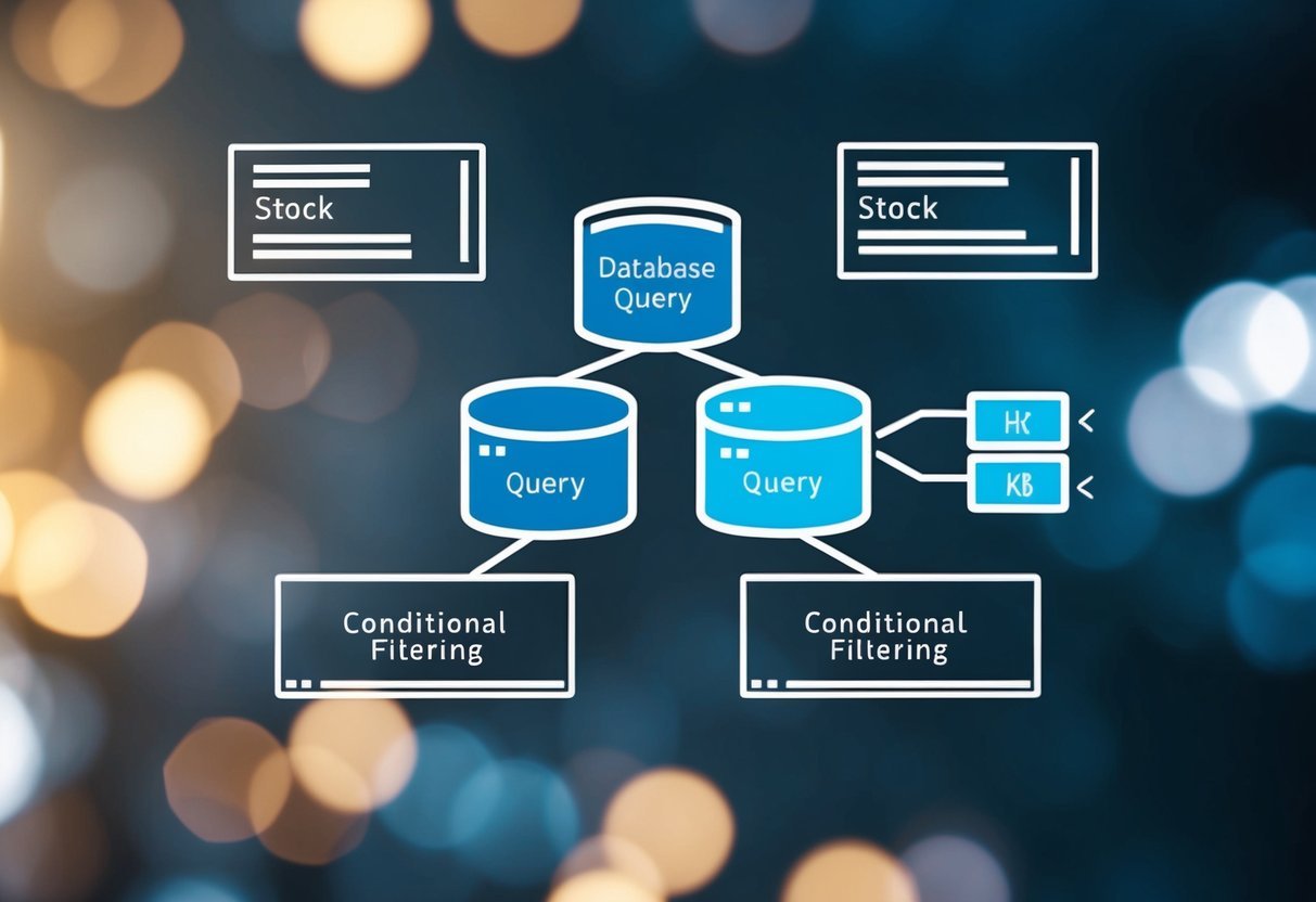
A database query diagram with nested subqueries and conditional filtering

Correlated subqueries play a crucial role in SQL for retrieving detailed data by processing each row individually.

These subqueries integrate seamlessly with various SQL clauses, impacting performance and efficiency.

Defining Correlated Subqueries

Correlated subqueries differ from conventional subqueries. They reference columns from the outer query, making them dependent on each row processed.

Such subqueries allow SQL to return precise datasets by matching conditions dynamically.

Commonly, these appear in the WHERE clause, enhancing the ability to filter results in SQL Server.

Correlated subqueries execute a query tied to the outer query’s current row. This execution relies on the values checked against the database at the time of the query.

Thus, they can be essential for tasks requiring detailed, row-specific data selections.

Performance Impact of Correlated Subqueries

While powerful, correlated subqueries can influence query performance.

Since they execute for each row processed by the outer query, they can lead to slower performance with large datasets. This occurs because SQL often runs these subqueries as nested loop joins, handling them individually for each row.

Using a correlated subquery efficiently requires careful consideration of data size and processing requirements.

Optimizing the outer query and choosing the correct clauses, like the FROM or WHERE clause, can mitigate these impacts.

For demanding processing, exploring alternatives or indexes might be useful to reduce load times and improve response efficiency.

Exploring Advanced Use Cases
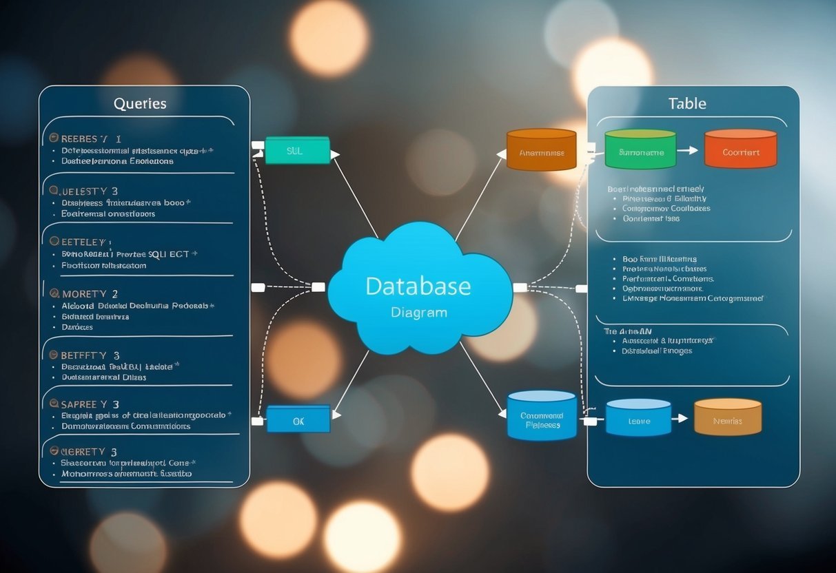
A database diagram with complex SQL queries and tables linked by advanced filtering conditions

SQL’s advanced filtering techniques, like EXISTS and NOT EXISTS, provide powerful ways to refine data queries. They help to handle complex filtering tasks by checking the presence or absence of records in subqueries.

These techniques are crucial when filtering based on conditions tied to related data in a user-friendly manner.

Filtering with Product Attributes

When dealing with product databases, filtering with attributes such as product_id or product_name is common.

The EXISTS operator can be used to determine if a product with specific attributes is available in another table.

For instance, querying if a product_id is linked to any orders, uses EXISTS in a subquery that checks the orders table for the presence of the same product_id. This ensures only products with existing sales appear in results.

Using NOT EXISTS, you can filter products that do not meet certain attribute conditions.

For example, filtering to find products that have never been sold involves checking for product_id values absent in the orders table. This technique helps businesses identify which items fail to convert to sales, aiding inventory management.

Scenario-Based Filtering Examples

In scenarios where inventory needs to be synchronized with sales data, EXISTS becomes a useful tool.

By filtering based on whether inventory items exist in sales records, analysts can spot discrepancies.

For instance, creating a query to list inventory items sold and ensuring that product_id matches between tables provides accurate sales insights.

NOT EXISTS is similarly valuable in filtering scenarios, such as finding products lacking a specific feature.

An example includes checking for product_name not listed in a promotions table, which informs marketing who can target these products for future deals.

Such precise filtering helps companies to refine their inventory and sales approach significantly.

For detailed tutorials on using the EXISTS operator, DataCamp offers useful resources on how to use SQL EXISTS.

SQL Server-Specific Filtering Features
A database query with SQL code, highlighting the use of EXISTS and NOT EXISTS for filtering data

In SQL Server, various advanced filtering functions are available to help manage and manipulate data efficiently. The EXISTS and NOT EXISTS operators are crucial in forming complex queries by filtering rows based on specified criteria.

Exclusive SQL Server Functions

SQL Server offers unique functions that enhance data filtering.

The EXISTS operator checks the presence of rows returned by a subquery. If the subquery finds records, EXISTS returns true, allowing retrieval of specific datasets.

Conversely, the NOT EXISTS operator is handy for excluding rows. It returns true if the subquery yields no rows, making it ideal for filtering out non-matching data.

This operator is particularly useful for larger tables and when handling NULL values since it avoids complications that may arise with other filtering techniques.

These operators play a critical role in improving query performance.

They simplify data management, making them essential tools in SQL Server operations.

By understanding and utilizing these advanced functions, users can effectively manage and analyze complex data sets with precision.

Frequently Asked Questions

A computer screen displaying SQL code with advanced filtering using EXISTS and NOT EXISTS

Understanding SQL filtering with EXISTS and NOT EXISTS involves comparing their use with other techniques like IN and JOIN. The performance and syntax differences can significantly impact query efficiency.

Can you compare the performance implications of using IN vs. EXISTS in SQL queries?

When deciding between IN and EXISTS, performance can vary.

Generally, EXISTS can be more efficient when dealing with subqueries that return larger datasets, as it stops processing once a match is found. IN might perform better with smaller datasets but can slow down with larger ones.

What are the practical differences between EXISTS and NOT EXISTS in SQL?

EXISTS checks for the presence of rows returned by a subquery. If at least one row exists, it returns TRUE.

In contrast, NOT EXISTS returns TRUE only if the subquery produces no rows. This difference is crucial when filtering datasets based on whether related records exist.

How do I correctly use the EXISTS clause in SQL with an example?

To use EXISTS, you embed it within a SQL query.

For example, you can select customers from a list where each has placed at least one order:

SELECT CustomerName 
FROM Customers 
WHERE EXISTS (
    SELECT 1 
    FROM Orders 
    WHERE Customers.CustomerID = Orders.CustomerID
);

In what scenarios should NOT EXISTS be used instead of a JOIN in SQL?

NOT EXISTS is preferable to JOIN when checking for records’ absence in a related table.

Use it when you need to find rows in one table that do not have corresponding entries in another. This approach can be more efficient than a LEFT JOIN followed by a NULL check.

How can one check for the absence of records in a SQL database using NOT EXISTS?

To verify a record’s absence, NOT EXISTS can be utilized.

For example, to find employees without orders:

SELECT EmployeeName 
FROM Employees 
WHERE NOT EXISTS (
    SELECT 1 
    FROM Orders 
    WHERE Employees.EmployeeID = Orders.EmployeeID
);
```Sure, I can help with that! Could you please provide the text that you would like me to edit?

### What are the syntax differences between IF EXISTS and IF NOT EXISTS in SQL?

The IF EXISTS syntax is used when dropping objects like tables or indexes to ensure they are present. 

Conversely, IF NOT EXISTS is used when creating objects only if they do not already exist. 

These commands help avoid errors in SQL executions when altering database objects.
Categories
General Data Science

The Importance of SQL in Data Science: Unveiling Its Crucial Role

Structured Query Language, commonly known as SQL, is the bedrock for data manipulation and retrieval in relational databases.

In the realm of data science, SQL’s significance cannot be overstated as it provides the foundational tools for data scientists to cleanse, manipulate, and analyze large sets of data efficiently.

The power of SQL lies in its capability to communicate with databases, allowing for the extraction of meaningful insights from raw data.

Its importance is recognized by both academia and industry, with SQL continuing to be a core component of data science education and practice.

A computer screen showing SQL queries and data visualizations

The versatility of SQL is showcased through its widespread application across various domains where data science plays a crucial role.

Data scientists regularly utilize SQL to perform tasks such as data cleaning, data wrangling, and analytics, which are essential for making data useful for decision-making.

Mastery of SQL gives data scientists the advantage of directly interacting with databases, thus streamlining the data analysis process.

As such, SQL serves as a critical tool for converting complex data into actionable knowledge, underpinning the development of data-driven solutions.

Understanding SQL is also crucial for the implementation of machine learning models, since SQL facilitates the construction of datasets needed for training algorithms.

The language’s relevance extends to the creation of scalable data infrastructures, further emphasizing its role as an enabler for the innovative use of data in science and technology.

With the increasing centrality of data in modern enterprises, SQL continues to be a key skill for data professionals aiming to deliver valuable insights from ever-growing data ecosystems.

Fundamentals of SQL for Data Science

A computer screen displaying SQL queries and data tables, with a book titled "Fundamentals of SQL for Data Science" open next to it

SQL, or Structured Query Language, is essential for manipulating and querying data in relational databases.

Data scientists utilize SQL to access, clean, and prepare data for analysis.

Understanding SQL Syntax

SQL syntax is the set of rules that define the combinations of symbols and keywords that are considered valid queries in SQL.

Queries often begin with SELECT, FROM, and WHERE clauses to retrieve data matching specific conditions.

The syntax is consistent and allows for a variety of operations on database data.

Data Types and Structures in SQL

SQL databases are organized in tables, consisting of rows and columns.

Each column is designed to hold data of a specific data type such as integer, float, character, or date.

Understanding these data types is vital, as they define how data can be sorted, queried, and connected within and across tables.

SQL Operations and Commands

A range of SQL operations and commands enables data scientists to interact with databases.

Common operations include:

  • SELECT: Extracts data from a database.
  • UPDATE: Modifies the existing records.
  • INSERT INTO: Adds new data to a database.
  • DELETE: Removes data from a database.

Each command is a building block that, when combined, can perform complex data manipulations necessary for data analysis.

Data Manipulation and Management

In the realm of data science, SQL is a cornerstone for effectively handling data. It empowers users to interact with stored information, making it a vital skill for data manipulation and management tasks.

Data Querying

SQL is renowned for its powerful querying capabilities.

By utilizing SELECT statements, data scientists can retrieve exactly the data they require from large and complex databases. The WHERE clause further refines this by allowing for precise filtering.

  • Retrieve data: SELECT * FROM table_name;
  • Filter results: SELECT column1, column2 FROM table_name WHERE condition;

Data Insertion

To add new records to a database, SQL employs the INSERT INTO statement.

This is crucial for expanding datasets in a systematic manner. Before analysts can query or manipulate data, it must first be properly inserted into the database.

  • Insert single record: INSERT INTO table_name (column1, column2) VALUES (value1, value2);
  • Insert multiple records: INSERT INTO table_name (column1, column2) VALUES (value1, value2), (value3, value4);

Data Update and Deletion

SQL commands UPDATE and DELETE play critical roles in maintaining database integrity and relevance.

The UPDATE statement is employed to modify existing records. Concurrently, DELETE is used to remove unwanted data, keeping databases efficient and up-to-date.

  • Update records: UPDATE table_name SET column1 = value1 WHERE condition;
  • Delete records: DELETE FROM table_name WHERE condition;

SQL commands for data manipulation are essential for managing the lifecycle of data within any database, ensuring that datasets remain current and accurate for analysis.

SQL in Data Analysis

SQL is a cornerstone in data analysis for its robust functionality in data manipulation and retrieval. It enables analysts to interact efficiently with large databases, making it indispensable for data-driven decision-making.

Aggregating Data

In data analysis, aggregating data is crucial to summarize information and extract meaningful insights.

SQL provides functions such as SUM(), AVG(), COUNT(), MAX(), and MIN() that allow users to perform calculations across rows that share common attributes.

Analysts rely on these aggregations to condense datasets into actionable metrics.

  • SUM() computes the total of a numeric column.
  • AVG() calculates the average value in a set.
  • COUNT() returns the number of rows that satisfy a certain condition.
  • MAX() and MIN() find the highest and lowest values, respectively.

Data Sorting and Filtering

To enhance the readability and relevance of data, data sorting and filtering are vital.

SQL’s ORDER BY clause sorts retrieved data by specified columns, either in ascending or descending order, aiding in organizing results for better interpretation.

The WHERE clause filters datasets based on specified criteria, thus enabling analysts to isolate records that meet certain conditions and disregard irrelevant data.

  • ORDER BY column_name ASC|DESC sorts rows alphabetically or numerically.
  • WHERE condition filters records that fulfill a particular condition.

Joining Multiple Data Sources

SQL excels at joining multiple data sources, a technique pivotal for comprehensive analysis when datasets are housed in separate tables.

By using JOIN clauses, one can merge tables on common keys, juxtaposing related data from various sources into a single, queryable dataset.

Types of joins like INNER JOIN, LEFT JOIN, RIGHT JOIN, and FULL OUTER JOIN give analysts the flexibility to choose how tables relate to one another.

  • INNER JOIN returns rows when there is at least one match in both tables.
  • LEFT JOIN includes all rows from the left table, with matching rows from the right table.
  • RIGHT JOIN and FULL OUTER JOIN operate similarly but with emphasis on the right table, or both tables, respectively.

Database Design and Normalization

Within the realm of data science, efficient database design and normalization are pivotal. They ensure the integrity and optimality of a database by organizing data to reduce redundancy and enhance data retrieval.

Schema Design

Schema design is the first crucial step in structuring a database. A well-planned schema underpins a database’s performance and scalability.

The goal is to design a schema that can handle a variety of data without inefficiency, which can be achieved through normal forms and normalization.

For example, a normalization algorithm plays a critical role in eliminating redundant data, ensuring schemas are free from unnecessary repetition.

Indexing

Indexing proves indispensable in optimizing data retrieval. It functions much like an index in a book, allowing faster access to data.

However, one must employ indexing judiciously. Over-indexing leads to increased storage and can negatively impact write operations performance, while under-indexing can leave the system sluggish during queries.

Mastering the use of indexes is a subtle art crucial for database efficiency, tying in closely with the schema to ensure a balanced and efficient database system.

SQL Optimization Techniques

Optimizing SQL is pivotal in data science to enhance query performance and ensure efficient data management. Rigorous optimization techniques are the backbone for responsive data analysis.

Query Performance Tuning

In query performance tuning, the focus is on framing SQL statements that retrieve results swiftly and efficiently.

Data scientists often use EXPLAIN statements to understand how the database will execute a query.

Additionally, avoiding unnecessary columns in the SELECT statement and using WHERE clauses effectively can lead to more focused and hence faster queries.

Efficient Data Indexing

Efficient data indexing is crucial for improving query performance.

By creating indexes on columns that are frequently used in the WHERE clause or as join keys, databases can locate the required rows more quickly.

It is important to consider the balance between having necessary indexes for query optimization and having too many, which may slow down insert and update operations.

Execution Plans and Caching

Understanding execution plans is key for identifying bottlenecks in query performance.

Data scientists can interpret these plans to modify queries accordingly.

Furthermore, implementing caching strategies where commonly retrieved data is stored temporarily can significantly improve query response time.

Servers can serve cached results for common queries instead of re-executing complex searches.

Integrating SQL with Other Tools

SQL’s versatility allows it to enhance data science processes when combined with other tools. It serves as a robust foundation for various integrations, enabling more sophisticated analysis and data management.

SQL and Spreadsheet Software

Integrating SQL with spreadsheet applications like Excel enables users to manage larger datasets that spreadsheets alone could handle inefficiently.

Functions such as importing SQL queries into a spreadsheet or using SQL to automate the manipulation of data in Excel provide a powerful extension to the spreadsheet’s native capabilities.

SQL and Programming Languages

SQL’s integration with programming languages such as Python or R amplifies data science capabilities.

For example, Python offers libraries like pandas for data analysis and sqlalchemy for database management. These libraries allow SQL queries to be executed directly from the Python environment. As a result, workflows are streamlined and complex data manipulations are enabled.

SQL in Business Intelligence Tools

In business intelligence (BI) platforms, SQL plays a critical role in querying databases and generating reports.

Platforms such as Tableau or Power BI utilize SQL to extract data. This allows users to create interactive dashboards and visualizations that support data-driven decision-making.

Data Security and SQL

Data security within SQL-driven environments is crucial for safeguarding sensitive information.

It ensures that data is accessible only to authorized users and is protected against unauthorized access and threats.

Access Control

Access control is the process of determining and enforcing who gets access to what data within a database.

SQL implements access control via Data Control Language (DCL) commands such as GRANT and REVOKE. These commands are used to give or take away permissions from database users.

Data Encryption

Data encryption in SQL databases involves transforming data into a secured form that unauthorized parties cannot easily comprehend.

Encryption can be applied to data at rest, using methods like Transparent Data Encryption (TDE). It can also be applied to data in transit with Secure Sockets Layer (SSL) or Transport Layer Security (TLS).

SQL Injection Prevention

SQL injection is a technique where an attacker exploits vulnerabilities in the SQL code layer to execute malicious queries.

Preventative measures include using parameterized queries and stored procedures, which help ensure that SQL commands are not altered by user input.

Running regular security audits and keeping systems updated with security patches are also key strategies for SQL injection prevention.

Frequently Asked Questions

A computer screen displaying SQL code surrounded by data science icons and charts

In the realm of data science, Structured Query Language (SQL) is integral for the efficient handling of data. This section aims to address some common inquiries regarding its importance and utility.

What role does SQL play in managing and querying large datasets for data analysis?

SQL is the standard language used to retrieve and manipulate data stored in relational databases.

It enables data scientists to handle large volumes of data by running complex queries and aggregations which are pivotal for data analysis.

How does knowledge of SQL contribute to the effectiveness of a data scientist’s skill set?

Proficiency in SQL enhances a data scientist’s ability to directly access and work with data.

This direct engagement with data allows for a more profound understanding of datasets, leading to more accurate analyses and models.

Why is SQL considered a critical tool for performing data manipulations in data science?

SQL is essential for data science tasks as it allows for precise data manipulations.

Through SQL commands, data scientists can clean, transform, and summarize data, which are crucial steps before any data analysis or machine learning can be applied.

How can SQL skills enhance a data scientist’s ability to extract insights from data?

SQL skills empower a data scientist to efficiently sort through and query data, enabling the extraction of meaningful insights.

These skills are vital for interpreting data trends and making data-driven decisions.

What are the advantages of using SQL over other programming languages in data-driven projects?

SQL’s syntax is specifically designed for managing and querying databases, making it more streamlined and easier to use for these tasks than general-purpose programming languages.

This specialization often results in faster query performance and reduced complexity in data-driven projects.

In what ways does the mastery of SQL impact the efficiency of data cleaning and preprocessing?

Mastery of SQL can significantly expedite data cleaning and preprocessing.

With advanced SQL techniques, data scientists can quickly identify and rectify data inconsistencies.

They can also streamline data transformation and prepare datasets for analysis in a more time-effective manner.

Categories
Uncategorized

Learning about Pandas to Concatenate Multiple Dataframes: A Quick Guide

Understanding Data Concatenation in Pandas

When working with data in Python, Pandas is a powerful library that helps in handling and analyzing data efficiently.

One crucial aspect of data manipulation in Pandas is the ability to concatenate multiple DataFrames.

The concat() function in Pandas allows users to combine two or more DataFrames. This can be done either vertically, stacking one on top of the other, or horizontally, merging them side by side.

This flexibility is vital for managing large datasets that need integration from various sources.

Axis Description
0 Concatenates along rows
1 Concatenates along columns

To avoid confusion while concatenating, ensure DataFrames have consistent indices and column names.

Misaligned data can lead to unexpected behavior or loss of information in the resulting DataFrame.

Here’s a simple example of using the concat() function:

import pandas as pd

df1 = pd.DataFrame({'A': [1, 2], 'B': [3, 4]})
df2 = pd.DataFrame({'A': [5, 6], 'B': [7, 8]})

result = pd.concat([df1, df2], axis=0)

The example above shows how to combine DataFrames by stacking them vertically.

Exploring more about this topic, one can refer to resources like the Pandas documentation and guides from sites like GeeksforGeeks.

Setting Up Your Environment for Pandas

To get started with Pandas, ensure that the necessary software is installed on your computer.

The primary software needed is Python along with the Pandas library. You can install it using pip:

pip install pandas

Once installed, you can import Pandas into your Python scripts:

import pandas as pd

Creating a Pandas DataFrame is a fundamental operation. A DataFrame can be created from a dictionary or a list. Here’s a simple example:

data = {'Name': ['Alice', 'Bob'], 'Age': [25, 30]}
df = pd.DataFrame(data)

For a comprehensive coding experience, consider using an Integrated Development Environment (IDE) like Jupyter Notebook or PyCharm. These environments provide code completion and visualization tools.

If Jupyter Notebook is preferred, install it using:

pip install jupyter

Basic Packages

It’s beneficial to have other essential Python packages like NumPy and Matplotlib. They enhance the functionality and performance of Pandas, especially in handling large datasets and visualizing data.

  • NumPy: Provides support for large arrays and matrices.
  • Matplotlib: Useful for plotting and graphing.

Virtual Environments are helpful in managing dependencies and keeping project-specific configurations isolated. Create a virtual environment with:

python -m venv env

Activate this environment before installing packages:

  • Windows: .envScriptsactivate
  • Mac/Linux: source env/bin/activate

By setting up these tools, you create a robust environment for working effectively with Pandas and large datasets.

Basics of Pandas DataFrames

Pandas DataFrames are central to data manipulation in Python. A DataFrame is essentially a table, similar to an Excel spreadsheet, consisting of rows and columns. Each column in a DataFrame is a Pandas Series, which represents one-dimensional data.

A DataFrame can be created in various ways, such as from a dictionary or a list. For example:

import pandas as pd

data = {'Name': ['Alice', 'Bob'],
        'Age': [25, 30]}
df = pd.DataFrame(data)

Pandas DataFrames come with indices, which are labels for rows. By default, these indices are numerical and start at zero, but they can be set to any value. Indices help in selecting and organizing the data.

Pandas allows for easy data manipulation, such as selecting, merging, and organizing the data. This can be done through various methods like concat(), merge(), and others. These operations are fundamental when working with multiple DataFrames.

Key Features:

  • Flexible Data Structures: Combine data from different sources effortlessly.
  • Powerful Indexing: Access and manipulate specific data easily.
  • Efficient Data Handling: Manage large datasets with ease.

Understanding these basics helps in efficiently utilizing Pandas for data analysis. With these tools, users can manage datasets smoothly, making Pandas a powerful ally in any data-driven task.

Concatenating DataFrames Vertically

Concatenating DataFrames vertically in Pandas allows users to stack data from different sources into one table. By using the right functions, such as pd.concat, data from different DataFrames can be efficiently combined, even when columns don’t perfectly align.

Using Concat() for Vertical Concatenation

The pd.concat function is the primary tool for combining DataFrames vertically. It stacks DataFrames along rows when axis=0 is used, making it ideal for merging datasets. For seamless integration, setting ignore_index=True ensures that the resulting DataFrame has a reset index.

When the DataFrames have differing column numbers, gaps may occur, resulting in NaN values for missing data.

This method allows for flexibility, handling datasets with varying structures. To append new data frames continuously, concat offers a robust solution without altering existing ones.

Using pd.concat guarantees a structured and efficient approach to managing and analyzing larger datasets.

Handling Missing Values and NaN

Vertical concatenation often introduces missing values, represented as NaN, when DataFrames have different columns. Addressing these NaNs is crucial for data integrity.

The pd.concat method inherently manages such discrepancies by adding NaN where necessary.

Data analysts can choose specific strategies to deal with these missing values. Options include filling them with a default value using fillna(), or executing data cleaning steps to drop irrelevant columns.

Proper handling of NaN ensures the resultant DataFrame remains useful for further analysis. This practice also aids in ensuring that analyses are based on complete and meaningful data sets, reducing the risk of errors in computations.

Concatenating DataFrames Horizontally

When working with multiple DataFrames in Pandas, combining them horizontally is often necessary. This method involves aligning DataFrames side by side, which can be efficiently done using Pandas’ tools.

Specifying Axis in Concat() Function

To concatenate DataFrames horizontally, the pd.concat() function is used with axis=1. Setting axis to 1 tells the function to add columns instead of stacking rows. This is essential when the goal is to expand the DataFrame width-wise.

Using the function is straightforward:

import pandas as pd

df1 = pd.DataFrame({'A': [1, 2], 'B': [3, 4]})
df2 = pd.DataFrame({'C': [5, 6], 'D': [7, 8]})

result = pd.concat([df1, df2], axis=1)

This command results in a DataFrame combining all columns from df1 and df2. Choosing the correct axis is crucial for achieving desired alignment and data structure.

Dealing with Duplicates in Columns

When DataFrames have common columns, concatenating them might result in duplicate columns. This is a critical aspect of horizontal concatenation.

To handle this, it’s advisable to first inspect and potentially rename or drop conflicting columns before using pd.concat().

If there are conflicting columns, Pandas will append a suffix to distinguish them:

df1 = pd.DataFrame({'A': [1, 2], 'B': [3, 4]})
df2 = pd.DataFrame({'B': [5, 6], 'C': [7, 8]})

result = pd.concat([df1, df2], axis=1)

This situation can cause confusion in data analysis. To avoid this, you can rename columns using DataFrame.rename() or choose columns carefully:

df2 = df2.rename(columns={'B': 'B_1'})
result = pd.concat([df1, df2], axis=1)

Being aware of column names and managing duplicates helps maintain organized and clear DataFrames.

Advanced Concatenation Techniques

Working with multiple DataFrames often involves advanced techniques to effectively manage and merge data.

Two important strategies include using hierarchical indexing for organizing data and joining DataFrames that do not share the same indices.

Hierarchical Indexing and MultiIndex

Hierarchical indexing, also known as MultiIndex, allows for more complex data organization within a DataFrame. This technique enables the use of multiple index levels on both rows and columns, creating a tree-like structure. It provides a way to label data uniquely across these levels.

By employing a MultiIndex, DataFrames can represent higher-dimensional data in a two-dimensional table format. This is especially useful when dealing with multi-dimensional arrays or when needing to summarize data at varying levels of granularity.

Pandas supports creating a MultiIndex using tuples or by converting existing columns into an index. Advanced data operations like slicing or reshaping become more straightforward when a hierarchical index is in place.

This method is often employed in datasets requiring multiple categories of classification.

Joining DataFrames with Different Indices

Joining DataFrames with different indices can handle complex merging tasks where direct alignment is necessary.

The DataFrame.join() method in Pandas supports alignment based on both index and columns, allowing for customized merging strategies.

This method can perform different types of joins, such as left, right, inner, or outer, specified by the how parameter.

When dealing with varied indices, it’s crucial to understand how these different types of joins will affect the resulting DataFrame structure.

For instance, an outer join merges data by including all indices from both DataFrames, filling in missing values where necessary.

On the other hand, an inner join keeps only the intersecting indices from both sets, ensuring that only common elements are merged. Understanding these concepts can greatly enhance data management and analysis capabilities when working with DataFrames.

Understanding Join Operations

Join operations in Pandas are powerful tools for combining data from multiple DataFrames. These operations allow users to align and merge datasets based on common columns or indices, enabling the seamless integration of related data.

Exploring Inner and Outer Joins

Inner joins are used to find the intersection between two DataFrames. It returns rows with matching values in both DataFrames, excluding non-matching data. This join is useful when the focus is on common elements, ensuring only overlapping information is retained.

An outer join ensures a comprehensive union of both DataFrames, including all rows from each, with NaNs filling in the gaps where there’s no match. This type of join is beneficial when all potential data points need consideration, even if they don’t perfectly align.

Here’s a quick comparison:

Join Type Output
Inner Join Only common data
Outer Join All data, with NaN for non-matches

Left and Right Joins Explained

A left join keeps all records from the left DataFrame and adds matching records from the right DataFrame. If no match is found, the result is filled with NaN.

This method is useful when the priority is maintaining the full dataset of the left DataFrame.

On the other hand, a right join does the reverse. It maintains all values from the right DataFrame, appending data from the left only where matches occur.

It is key when the right DataFrame serves as the primary dataset.

Leveraging Keys and Indices in Concatenation

Keys and indices play a crucial role when using the concat() function in Pandas to join multiple DataFrames. They offer more control over how the data is structured after concatenation.

By specifying keys, one can add a level to the resulting DataFrame’s index, which can be particularly useful for tracking the origin of each DataFrame.

When concatenating n DataFrames, the ignore_index parameter becomes handy if there’s a need to reset indices.

Setting ignore_index=True results in a continuous index for the combined DataFrame, without considering the original indices.

Sometimes there is a need to merge DataFrames multiple times or in a specific order.

In such scenarios, using the reduce method from Python’s functools module combined with a concat() can be efficient.

This approach applies concatenation iteratively over a list of DataFrames.

For enhanced indexing control, the levels and keys arguments allow for detailed customization.

When the concat() function uses levels, it helps in creating multi-index DataFrames with defined levels based on the concatenated data.

The ability to use keys effectively becomes crucial when working with complex datasets. It ensures clarity and helps maintain data integrity, significantly aiding in post-concatenation data manipulation and analysis.

More detailed insights and examples on using keys and indices in concatenation can be found at SQLPey.

Merging DataFrames: Merge() vs Concat()

When working with pandas, combining dataframes is a common task. The merge() and concat() functions are essential tools, each serving different purposes.

Using Merge() for Complex Joins

The merge() function in pandas is highly versatile for combining dataframes based on common columns or indices. It resembles SQL join operations, allowing for complex relational data manipulations.

For instance, users can specify inner, outer, left, or right joins using the how parameter. This flexibility is critical when aligning rows from two dataframes based on shared keys.

The ability to align data across multiple columns makes merge() valuable when precise row matching is needed.

In addition, users can merge dataframes on their index by setting left_index=True and right_index=True.

More details and examples can be found on Real Python.

Comparison of Merge() and Concat()

While merge() is designed for joining dataframes based on shared keys, concat() is used for either appending or stacking dataframes. It supports operations along rows (axis=0) or columns (axis=1).

Choosing between these depends on the task. concat() can quickly stack data without needing a shared key.

Another difference is how they handle duplicates. merge() can filter rows based on duplicates or data overlap, while concat() will include all data by default.

This makes concat() ideal when simply extending a dataset. For detailed handling of different concatenation logic, pandas documentation offers more guidance.

Practical Examples and Use Cases

In data analysis, it is common to concatenate DataFrames. This means combining two or more data tables, either vertically or horizontally, depending on the need.

For example, if you have monthly sales data in separate DataFrames, you can stack them vertically to create a complete dataset for the year.

To use the concat() function, place the DataFrames in a list and call pd.concat(). This function allows control over how data is joined, such as deciding the column or row axis.

Here’s a simple example:

import pandas as pd

df1 = pd.DataFrame({'A': [1, 2], 'B': [3, 4]})
df2 = pd.DataFrame({'A': [5, 6], 'B': [7, 8]})

result = pd.concat([df1, df2])

Output:

A B
1 3
2 4
5 7
6 8

Using concat() is effective for merging datasets with similar structures. If the DataFrames have different columns, concat() can still align them by adding NaN in missing spaces.

When combining DataFrames with different indexes or needing to eliminate duplicates, one can also use the join or merge functions, depending on the specific task and data structure requirements.

To learn about concatenating DataFrames, you can explore resources like the Pandas concat() Function Tutorial.

This versatility makes concat() an essential method for data scientists dealing with large datasets across multiple sources.

Optimizing Performance for Large DataFrames

Multiple large data tables merging into one, symbolizing optimization and learning about Pandas to concatenate dataframes

Pandas offers efficient ways to handle large DataFrames. When merging or concatenating multiple DataFrames, performance is key. Using the right techniques can make a big difference.

Avoid Repeated Concatenations
Concatenating a list of DataFrames at once is more efficient than doing it one by one. For large data, using pd.concat([df1, df2, df3]) is recommended.

Index Management
The index plays an important role when merging. Always reset the index when needed, such as with df.reset_index(drop=True). This ensures alignment and can boost performance. Read more about tips from this article.

Optimized DataFrame Usage
When multiple DataFrames have to be merged, using efficient methods is vital. Consider using lambda and reduce approaches for cleaner code and performance gains.

Memory Management
Large DataFrames consume significant memory. Efficient memory usage can be managed by using appropriate data types. For instance, using int32 instead of int64 when the size allows. It reduces memory footprint, making operations faster.

Built-in Functions
Pandas provides built-in functions like concat() for combining DataFrames efficiently. These can be harnessed by understanding their nuances and applying tricks to speed up data analysis. Insights on these functions can be found in various resources, such as this guide.

Best Practices and Tips

Multiple pandas learning to concatenate dataframes in a classroom setting with a chalkboard and teacher

When working with multiple DataFrames in Pandas, it is important to follow best practices to ensure seamless data handling.

Use the Right Method:
Choose between concat() and merge() based on your needs. Use concat() to stack DataFrames along a particular axis. Use merge() when you need to combine DataFrames on a key or common column.

Handle Indexes Effectively:
While using pandas concat, set ignore_index=True if you do not want the old index to be retained. This helps in resetting the index of the new DataFrame, making it more readable.

Check DataFrame Structures:
Before concatenating, ensure that DataFrames have compatible structures. This means columns should be in the correct format and order.

Memory Management:
Large DataFrames can consume lots of memory. Consider optimizing your data types or processing data in chunks. This approach can prevent memory overflow.

Use Meaningful Column Names:
Avoid duplicate column names after a merge. Differently labeled columns result in easier debugging and data comprehension.

Test with Small DataFrames First:
Before applying operations on large datasets, practice with smaller examples to catch potential issues without consuming excessive resources.

Frequently Asked Questions

A panda mascot surrounded by multiple interconnected dataframes

This section addresses common questions about concatenating and merging DataFrames in Pandas. It covers methods for combining data vertically and horizontally, explains differences between operations, and suggests best practices.

How can I merge two DataFrames in Pandas based on a common column?

To merge two DataFrames using a common column, the merge() function is used. It combines DataFrames on specific key columns and offers various types of joins such as inner, outer, left, and right. For more information, refer to the Pandas documentation on merging.

What is the difference between join and merge operations in Pandas?

In Pandas, merge allows combining DataFrames based on key columns, much like SQL join operations. It can use multiple keys. The join method is specifically for DataFrame objects and connects DataFrames along their index. Learn more about these operations in this documentation.

How do you vertically concatenate two DataFrames with different columns in Pandas?

To vertically concatenate DataFrames with differing columns, use the concat() function. By default, it matches columns by name and fills in missing values with NaN. For a detailed explanation, see this guide.

Is there a way to concatenate multiple DataFrames horizontally using Pandas?

Yes, Pandas provides the concat() function to join DataFrames horizontally by setting the axis parameter as 1. This is useful for side-by-side data alignment. For more details on this process, examine this information.

What are the best practices for using a for loop to concatenate multiple DataFrames in Pandas?

When using a for loop to concatenate, append each DataFrame object to a list and then use pd.concat on the list. This approach is both efficient and scalable. More about this technique can be found in this Stack Overflow discussion.

How to combine two Pandas DataFrames with a different number of rows?

Combining two DataFrames with different row counts can be done with the concat() function.

This function aligns the DataFrames based on the index, and any extra data is filled with NaN by default.

For further exploration, check this guide.

Categories
Uncategorized

Learning About Python Scope: A Comprehensive Guide

Understanding Python Scope Fundamentals

Python scope determines where variables can be accessed within the code. It is essential for developers to grasp how Python handles variable visibility by using different scopes, following the LEGB rule.

The Four Scopes in Python: LEGB

In Python, variables can exist in four main scopes: Local, Enclosing, Global, and Built-in. These scopes are often referred to using the acronym LEGB. This structure defines the sequence that Python follows when checking where a variable is defined or can be accessed.

  • Local Scope: Variables within a function. They can only be accessed inside that function.
  • Enclosing Scope: This applies to nested functions. Variables in the outer function are accessible to the inner function.
  • Global Scope: These variables are defined at the top level and are accessible throughout the module.
  • Built-in Scope: Contains special Python-provided functions and names that are always available.

Understanding these scopes ensures that developers know where and how variables can be accessed in a program. For detailed insights, explore the LEGB Rule in Python Scope.

Variable Scope and Accessibility

The scope affects a variable’s accessibility, meaning where it can be used in the program.

For instance, local variables are restricted to the block they are created in, such as a function or loop. This ensures variables don’t interfere with others outside their scope.

With global variables, accessibility extends to the entire module. If accessed within a function, Python first looks for local variables before searching globally. The rules of accessibility defined by LEGB help avoid conflicts and unexpected errors in the code.

By following the principles of Python scope, programmers can manage variables effectively, preventing unintended changes in data and maintaining code clarity.

Global and Local Scopes Explained

Python’s scope rules determine where variables can be accessed within the code. Understanding these scopes is crucial for managing variables effectively and avoiding errors.

Defining Global Scope

In Python, the global scope refers to variables that are declared outside any function. These variables are accessible from any part of the code, both inside and outside functions. Global variables can be useful when the same data needs to be accessed throughout a program. For example, setting a variable like config = True outside a function makes config available everywhere.

However, modifying global variables inside functions requires the global keyword. This tells Python to use the variable from the global scope, instead of creating a new local one. For instance, updating a variable within a function would involve declaring it as global variable_name. Though global variables offer flexibility, overusing them can lead to issues with code readability and debugging.

Understanding Local Scope

Local scope refers to variables defined within a function. These variables exist only during the function’s execution and cannot be accessed outside of it. This isolation helps prevent conflicts with variables in other parts of the program.

If a variable like total = 10 is created inside a function, it is a local variable.

Each time a function is called, its local scope is created anew, ensuring that variables do not overlap between calls. This makes local variables ideal for temporary data that is specific to a function’s task. Using local variables keeps the program organized, as they are confined to the function in which they are declared, enhancing modularity and maintainability. For more on local scope, explore the concept on the Programiz site.

The Global Keyword in Depth

The global keyword in Python is essential for modifying variables outside their local scope. It allows programmers to alter global variables from within functions, impacting how data is organized and accessed across the program.

Usage of the Global Keyword

In Python, the global keyword is used within a function to change variables at the global scope. This means variables can be modified outside their local environment, which is typically restricted.

Using global, a function can create or alter global variables. This is useful when a variable needs to be changed in multiple functions or modules. Code examples, like those found in examples at W3Schools, demonstrate how a global declaration can alter a global variable from within a function.

The global keyword ensures that when a variable is called, Python recognizes it as global. This avoids confusion with variables that might share the same name but are local to other functions. Examples show it simplifies data management, though care is needed to prevent unintended changes.

Implications of Global Variable Assignment

Assigning variables as global means storing them in the global namespace. This impacts how variables are accessed throughout the program.

Global variables can be used by any function, making them powerful but also posing risks.

Global variables can lead to increased program complexity. If many functions modify the same global variable, it becomes difficult to track changes and debug issues. Solutions may include limiting the use of global state or isolating global variables to key functions.

It’s also advisable to document when and why global variables are used. This helps maintain clarity in codebases, as seen in in-depth discussions of global scope. Properly used, the global keyword balances accessibility and control within Python programs.

Delving Into Enclosing and Nested Scopes

Enclosing and nested scopes are crucial in Python programming. They determine how variables are accessed within functions and impact code organization. Understanding these concepts helps avoid errors and makes the code cleaner.

Nested Functions and their Scopes

Nested functions occur when a function is defined inside another function. In Python, this structure allows the inner function to access variables in the outer function’s scope. This is known as a nested scope. These inner functions can modify or use the surrounding variables, enabling more complex and organized code.

Nested functions are particularly useful for closures, which capture and remember values from their enclosing function even after the outer function has finished executing.

Nested scopes follow Python’s LEGB rule, prioritizing Local, Enclosing, Global, and Built-in scopes. It is essential for programmers to understand how this hierarchy affects variable access.

By using nested functions, developers can hide details and create more modular code, enhancing readability and maintainability.

Enclosing Scope Mechanics

The enclosing scope refers to the environment a nested function inherits from its containing function. It allows variables from the outer function to be used within an inner function without needing to pass them as arguments.

This capability is established through Python’s nonlocal keyword, which enables the inner function to modify variables from its enclosing scope.

Enclosing scopes are significant as they allow maintaining state across function calls with minimal overhead, often used in decorator functions or when defining callbacks.

Recognizing the enclosing scope helps in debugging scope-related issues by clarifying where variables are defined and modified. If a variable isn’t found in the local scope, Python automatically checks the enclosing scope level, providing a flexible variable access system for complex programs.

The Nonlocal Keyword and Its Use Cases

The nonlocal keyword in Python is crucial for managing variable scopes, especially in nested functions. It allows variables to be shared across these nested scopes without affecting global variables.

When to Use Nonlocal Keyword

In Python, the nonlocal keyword is used within nested functions when there is a need to modify a variable defined in an enclosing scope. This is important when a function needs to modify a variable from its enclosing function without making it a global variable.

For example, in a function-within-a-function setup, if the inner function needs to update a counter variable from the outer function, nonlocal can be employed. By doing so, the outer function’s state can persist across multiple calls to the inner function.

When the nonlocal keyword is used, Python searches for the variable in the nearest enclosing scope rather than the global scope, enhancing efficiency and clarity in code design.

Differences Between Nonlocal and Global

The distinction between nonlocal and global is found in their scope and usage. While nonlocal is used for variables within nested functions, global refers to variables at the module level.

Nonlocal targets a nested scope, specifically for modifying variables in an enclosing function’s local scope. This helps in cases where a variable must not be shared at the global level yet should be accessible across nested functions.

On the other hand, global makes a variable accessible throughout the entire module. If a variable needs to be accessed and modified everywhere in a program, it should be declared as global. The choice between the two keywords depends on whether the variable interaction is necessary at the module level or just between nested function scopes.

Python Built-In Scope and Builtin Functions

Python built-ins are core elements of the language, available without the need for user-defined declarations. Functions like print() are fundamental tools in Python programming, aiding in tasks from data output to built-in variable management. Understanding the scope of these functions helps in efficient programming.

Scope of Python Built-In Functions

In Python, the built-in scope caters to a set of functions readily available to use in any part of the program. These functions operate at the highest level of namespace, allowing them to be accessed without any prefixes. The built-in scope includes essential functions such as print(), len(), and input(), providing basic capabilities like displaying output, measuring the length of objects, and taking user input.

Built-in functions are accessible across all code since they are part of Python’s core library. This universality ensures that developers can freely use these functions without requiring imports. Built-in functions play a central role in making Python a user-friendly and efficient programming language.

List of Python Built-Ins

Below is a list of some key built-in functions in Python:

  • print(): Outputs data to the console.
  • len(): Returns the number of items in an object.
  • range(): Generates a sequence of numbers.
  • int(), str(), float(): Convert between data types.
  • input(): Captures user input from the console.

These functions are part of the built-in scope in Python, which allows them to be utilized easily and efficiently in various programming scenarios. Understanding these built-ins enhances the programmer’s ability to interact with and manipulate data effectively.

Scope-Related Keywords in Python

Understanding scope-related keywords in Python is crucial for managing where variables and functions can be accessed. These keywords, such as global and nonlocal, play a vital role in the language’s scoping rules. They affect how variable names are resolved and how they interact with different scopes and namespaces.

Global and Nonlocal Keywords

In Python, the global keyword allows variables to be accessed at a global level, even if they are set within a function. Without this keyword, a variable assigned within a function is local by default. This means it can’t change a variable with the same name outside the function.

For example, using global x sets x as a global variable inside a function, allowing it to be accessed or altered outside the function block as well.

The nonlocal keyword, meanwhile, is used for enclosing scopes in nested functions. It allows variables in an enclosing (but not global) scope to be bound to the new value. This helps manage nested function scenarios where neither the local nor global scope is appropriate.

Implications for Variable Binding

The usage of global and nonlocal significantly affects variable binding in Python. When employed, these keywords override the default behavior of variables being bound to local scopes within functions and lambda expressions.

This has direct implications for how code executes and interacts with different namespaces. It allows precise control over variable accessibility and lifetime.

For instance, using global or nonlocal can prevent common pitfalls related to unintended variable shadowing or scope leaks, facilitating clearer and more predictable code behavior.

Correct usage of these keywords is essential for effective manipulation of variable lifetimes and namespaces in Python programming.

Managing Namespaces and Variable Scope

Understanding the interaction between namespaces and variable scope helps in efficiently organizing a Python program. This involves distinguishing between global and local namespaces, and knowing the operations that can be performed.

Global vs Local Namespaces

In Python, the global namespace consists of all the identifiers defined at the top level of a module. These can include functions, classes, and variables.

This namespace is created when the module loads and can be accessed from any part of the program.

On the other hand, a local scope is specific to a function. When a function is called, it creates its own local namespace. Variables in this scope are local to the function and cannot be accessed outside of it.

Understanding the difference between these scopes is crucial for managing complex programs and ensuring variables are used correctly.

Python Namespace Operations

Python provides several operations to interact with namespaces. Functions like globals() and locals() can be used to access dictionaries representing the current global and local namespaces, respectively.

These functions are useful for examining or debugging variable values at different scope levels.

Additionally, dir() can be used to list the variables in a namespace.

Knowing these operations allows programmers to effectively manage and manipulate variables, ensuring they are used as intended and avoiding errors.

Organizing code around well-defined scopes leads to clearer and more maintainable Python programs.

Function and Class Scope in Python

In Python, the scope determines the accessibility and lifetime of variables. When working with functions and classes, understanding scope is key to managing variable visibility and avoiding conflicts.

Scope within Function Definitions

In Python, variables defined inside a function have local scope. These variables are only accessible within the function itself.

When the function is executed, Python creates a new, temporary scope that contains these local variables. Once the function exits, the local scope is destroyed, and the variables no longer exist.

Python applies the LEGB (Local, Enclosed, Global, Built-in) rule to resolve variables. This means that if a variable name is not found in the local scope, Python looks in enclosing scopes, then global, and finally built-in.

This structure allows functions to effectively manage data locally without interfering with other parts of the code. It’s important to remember that variables with the same name outside the function are treated as separate entities and can hold different values.

Understanding Class Scope

Like functions, classes in Python also have their unique scope, commonly referred to as the class scope.

Class variables are defined within the class and are shared among all instances of a class. They maintain a single copy of each variable, which helps in saving memory and ensuring consistent behavior.

Instance variables, on the other hand, belong to individual objects of the class. They are defined within methods using the self keyword, allowing each instance to maintain its unique state.

In Python 3, understanding the difference between class and instance variables is crucial for effective object-oriented programming.

It’s also significant to note the distinction between Python 2 and Python 3 in handling classes. Python 3 uses new-style classes by default, which brings additional features and improvements.

Advanced Scope Concepts and Closure

Advanced scope concepts in Python include the use of closures and how scope rules apply to features like list comprehensions and lambda expressions. Understanding these aspects can enhance code efficiency and behavior encapsulation.

Closures and Its Relation to Scope

In Python, a closure occurs when a function is defined inside another function and retains access to the variables from the outer function, even after the outer function has finished executing.

These are often used to encapsulate functionality and can keep track of the context in which they were created.

Closures differ from global variables as they do not expose internal states, aligning them closely with the concept of private methods in object-oriented programming.

For instance, a closure can encapsulate a variable using nested functions, allowing it to manipulate the outer scope from within the nested one.

This ability to bind data to function logic gives closures a powerful role in maintaining cleaner and more modular code structures.

Scope in List Comprehensions and Lambda

List comprehensions and lambda expressions bring unique interactions with scope in Python.

In list comprehensions, a new scope is created that protects variables defined within from affecting the variables outside of it. This feature prevents variables in comprehensions from overwriting existing ones.

On the other hand, lambda functions follow typical scope rules where they can access variables from their nonlocal environment, similar to closures.

While lambda allows concise and inline function definition, it’s crucial to understand that it maintains access to variables present in enclosing scopes at the time of its definition.

Understanding how lambda and comprehensions handle variable scopes helps in writing concise and effective code fragments.

Handling Scope-Related Errors in Python

A person studying Python code, encountering and resolving scope-related errors

When working with Python, scope-related errors can disrupt code execution. Common issues include UnboundLocalError and variable shadowing. Each of these errors has specific causes and solutions that can help avoid confusion in variable usage.

UnboundLocalError and Resolution

An UnboundLocalError often occurs when a local variable is referenced before it has been assigned a value. This happens frequently in functions where a variable is both read and assigned, but Python cannot identify which scope the variable belongs to.

To resolve this, ensure all variables are initialized before usage. The LEGB Rule can clarify which variable is being accessed.

Use the global or nonlocal keyword when a function needs to modify a variable outside its local scope. This can prevent most errors related to scope misunderstandings.

Variable Shadowing and Best Practices

Variable shadowing occurs when a local variable has the same name as a variable in an outer scope. This can cause confusion and lead to unintended behaviors because the local variable “shadows” the outer one, making it inaccessible within the function.

To avoid this, choose distinct names for local and global variables. Follow best practices by using descriptive names that reflect the variable’s purpose.

Be cautious when modifying global variables within functions. One suggestion is to use encapsulation by wrapping variables and related functions in classes to manage state more consistently.

Adhering to these practices can reduce errors linked to shadowing.

Python Scope and Memory Management

A python snake slithers through a forest, surrounded by floating memory management icons

In Python, the relationship between scope and memory management is vital. It affects how variables are stored and reclaimed, ensuring efficient use of resources. This involves garbage collection and variable lifespan, both influenced by scope rules in a Python program.

Scope’s Role in Garbage Collection

Garbage collection in Python helps automatically manage memory by deleting unused objects. Scope is key because it defines where variables are accessible.

When objects go out of scope, they lose references and become eligible for garbage collection.

For example, within a function, variables are local. Once the function ends, these variables often lose their references. This triggers the garbage collection system, which removes them to free up memory.

Effective scope management thus aids in optimizing memory usage.

The main program often involves several functions and classes. Each has its own scope. Being aware of these scopes helps the Python interpreter efficiently manage memory, reducing the likelihood of memory bloat.

Impact of Scope on Variable Lifespan

A variable’s lifespan is directly related to its scope. Variables defined in the global scope exist for the life of the Python program.

Meanwhile, local variables within a function are short-lived. Their lifespan ends when the function completes execution.

Temporary variables, often seen within loops or smaller blocks, have even shorter lifespans. They are frequently used and discarded, ensuring efficient memory use.

By managing these different scopes effectively, programmers can ensure variables are only active when needed.

Such controls help manage memory usage by the Python interpreter, ultimately improving a program’s efficiency.

Frequently Asked Questions

A computer screen displaying a webpage with a list of frequently asked questions about learning Python scope, surrounded by open books and a cup of coffee

Python’s scope rules define how variable names are resolved in code blocks like functions, loops, and conditions. Understanding these aspects is crucial for writing effective Python programs.

What are the different types of scopes available in Python?

Python uses the LEGB rule, which stands for Local, Enclosing, Global, and Built-in scopes. Local scope refers to variables defined within a function. Enclosing scope is relevant to nested functions. Global scope applies to variables declared outside any function. Finally, built-in scope includes names preassigned in Python’s modules. These scopes impact how variables are accessed and modified.

How does the local scope work in Python functions?

Local scope is specific to the block of code within a function. Variables declared here can only be accessed inside the function where they are defined.

Once the function execution completes, the allocated local memory is freed. This allows functions to have temporary data storage that does not interfere with other parts of the program.

Can you explain the concept of global scope and its usage in Python?

Global scope refers to variables defined outside of any function or class, making them accessible throughout the entire module.

To modify a global variable inside a function, the keyword global must be used. This allows the function to refer to the global variable instead of creating a new local one with the same name.

What is an enclosing scope, and how is it relevant in nested functions in Python?

Enclosing scope, also known as non-local or outer scope, occurs when there is a nested function. This scope pertains to variables that are in the parent function of the current function.

Using the nonlocal keyword, a variable in this scope can be accessed and modified within a nested function.

How does variable scope within loops and conditional constructs behave in Python?

Variables in loops and conditional statements follow the block scope rules. If a variable is defined within a loop or a condition, it is local to that block.

However, in Python, if a variable is assigned in a loop and accessed later outside of that loop, it retains its value from the last loop iteration.

What are the general rules that govern the scope of variables in Python programming?

Variables follow the LEGB rule.

Names are resolved by checking the local scope first, then the enclosing scope, followed by the global and built-in scopes.

If a variable is not found in these scopes, Python raises a NameError.

This structure ensures clear and predictable behavior for variable resolution.

Categories
Uncategorized

Learning T-SQL – Indexes: Mastering Efficient Data Retrieval

Understanding Index Basics

Indexes play a crucial role in SQL Server performance. They are designed to speed up data retrieval by providing a fast way to look up and access rows in a table.

An index in a database works like an index in a book. It allows you to quickly find the data you’re looking for without scanning every row in a table. This is especially useful in large datasets.

There are two main types of indexes in SQL Server: clustered and non-clustered indexes. A clustered index sorts the data rows in the table based on the index key. Each table can have only one clustered index because it directly orders the data.

Non-clustered indexes do not affect the order of the data in the table. Instead, they create a separate structure that references the storage of data rows. Each table can have multiple non-clustered indexes, offering different paths to data.

Proper indexing can significantly improve query performance. It helps the SQL Server quickly locate and retrieve the required information, reducing the time and resources needed for queries. Without indexes, the server might need to perform full table scans, which are often slow and inefficient.

However, indexing should be done carefully. While indexes improve data retrieval speeds, they can also slow down data modification operations like inserts, updates, and deletes. It’s important to balance between the number and types of indexes and the overall performance needs.

Indexes are a key aspect of Transact-SQL. Having a solid grasp of how they work can greatly enhance one’s ability to optimize and manage database performance.

Types of Indexes in SQL Server

Indexes in SQL Server enhance data retrieval efficiency, offering diverse options to cater to different requirements. This guide covers clustered, nonclustered, unique, columnstore, filtered, and special indexes like spatial and XML indexes.

Each type serves specific use cases, enabling optimal query performance and storage management.

Clustered Indexes

A clustered index determines the physical order of data in a table. Each table can have only one clustered index because the rows are physically sorted based on this index.

Clustered indexes are particularly useful for columns frequently used in range queries, as they store data rows in continuous blocks. This setup optimizes read performance, especially when accessing a large chunk of sequential data.

Typically, primary keys are created as clustered indexes unless specified otherwise. By organizing data pages sequentially, clustered indexes enhance retrieval speeds. However, inserting new rows might require adjusting the physical order, which can lead to more disk operations if not managed carefully.

Nonclustered Indexes

Nonclustered indexes create a separate structure from the data rows, containing a copy of selected columns along with pointers to the corresponding data records. They are beneficial for speeding up search queries that don’t align with the row order.

Multiple nonclustered indexes can be created on a table for different queries, providing versatility in accessing data.

The main advantage of nonclustered indexes is their ability to target specific queries without rearranging the physical data. They shine in query scenarios that benefit from quick lookups but also can increase storage requirements and slightly impact data modification speeds due to the maintenance of additional index structures.

Unique Indexes and Constraints

Unique indexes ensure that no duplicate values exist in the index key column or columns. When a unique index is defined, SQL Server enforces a unique constraint automatically, adding data integrity by ensuring each record maintains uniqueness.

Unique indexes are ideal for columns like email addresses, usernames, or other fields where duplicates should be avoided. While they prevent duplicates, unique indexes can also enhance query performance by offering efficient lookups and joins.

Implementing them may require careful planning, especially if modifications or deletions are frequent, since they enforce a strict constraint on the dataset.

Columnstore Indexes

Columnstore indexes are designed for efficient storage and retrieval of large volumes of data, particularly within data warehousing scenarios.

Rather than storing data row-by-row, columnstore indexes keep each column in a separate page. This format allows for high compression rates and rapid aggregate calculations, enabling faster query performance on large datasets.

They are suited for analytical queries where reading and processing large data sets is crucial. Columnstore indexes provide impressive compression, reducing I/O and improving query speed significantly. However, they might not be suitable for OLTP systems where quick single-row access and frequent updates are a priority.

Filtered Indexes

Filtered indexes are nonclustered indexes with a WHERE clause. This option allows indexing a portion of the data, making them cost-effective and efficient for queries that only access a small subset of data.

By including only relevant data, filtered indexes reduce storage space and improve performance by minimizing the data processed during queries.

Businesses can benefit from filtered indexes when dealing with frequently queried subsets, such as active orders in an order history database. Their use should be carefully considered, as they won’t be useful for queries outside their defined filter. Properly applied, they can significantly enhance query speeds while conserving resources.

Spatial and XML Indexes

Spatial indexes optimize queries involving spatial data types like geography and geometry. These indexes enable efficient spatial queries and spatial join operations.

For applications requiring location-based data manipulations, spatial indexes reduce processing time and improve performance significantly.

XML indexes enable efficient handling and querying of XML data stored in SQL Server. By organizing the XML data for rapid retrieval, these indexes are essential for developers dealing with large XML documents.

The right use of spatial and XML indexes can streamline complex query operations, making them indispensable in specialized database applications.

Creating and Managing Indexes

Indexes in T-SQL play a critical role in enhancing database performance. By properly creating, altering, and dropping indexes, a database can efficiently retrieve and update data.

Creating Indexes with T-SQL

Creating indexes in T-SQL involves defining the type of index you want, such as clustered or non-clustered.

A clustered index sorts the data rows in the table based on the index key. It is created using the CREATE CLUSTERED INDEX statement. For example, to create a clustered index on a column, the syntax would be:

CREATE CLUSTERED INDEX index_name ON table_name (column_name);

A non-clustered index creates a separate structure to hold the index on the data. It is useful for columns that are not the primary key. Here’s how to create one:

CREATE NONCLUSTERED INDEX index_name ON table_name (column_name);

Considerations while creating indexes should include the column’s data type and expected query patterns to maximize performance.

Altering Existing Indexes

Altering indexes might be necessary to modify their properties or improve efficiency.

While T-SQL itself doesn’t provide a direct ALTER INDEX command for changing an index’s properties, users often use DROP and CREATE commands together. This involves dropping an existing index and creating it again with the new configuration.

Sometimes, to add or remove columns from an index, the ALTER TABLE command can be valuable in modifying the table structure to accommodate index changes. This two-step process ensures that the index aligns with any changes in table design or usage requirements.

Dropping an Index

Dropping an index is essential when it becomes inefficient or is no longer needed. The DROP INDEX command is used for this purpose. For example:

DROP INDEX table_name.index_name;

It is crucial to assess the impact of dropping an index to avoid performance degradation. Removing unnecessary indexes can free up resources and reduce overhead caused by index maintenance.

It’s advisable to analyze query performance and use tools like SQL Server Management Studio for insights before deciding to drop an index.

Unique Indexes: Improving Data Integrity

Unique indexes play a crucial role in maintaining data integrity within a database. By ensuring that each value in a column is unique, they prevent duplicate entries. This feature is especially useful in columns where each entry must be distinct, like employee IDs or email addresses.

For enforcing data uniqueness, unique constraints and unique indexes work hand in hand. A unique constraint is a rule applied to a column or a set of columns, and the unique index is created automatically to support this rule. Both collaborate to maintain database accuracy and consistency.

A unique index can be either clustered or non-clustered. A unique clustered index physically arranges the data in a table based on the unique key. This organization speeds up data retrieval and ensures that index maintenance aligns with the table data’s order.

Here’s a simple list of benefits provided by unique indexes:

  • Enhanced data accuracy
  • Improved query performance
  • Prevention of duplicate entries

Creating these indexes involves a T-SQL command that looks like this:

CREATE UNIQUE INDEX index_name
ON table_name (column_name);

Using unique indexes effectively requires understanding the table’s purpose and usage patterns. They are best applied to fields where the uniqueness of data greatly influences the database’s integrity. For more detailed information, visit T-SQL Fundamentals.

Index Architecture and Index Keys

SQL Server uses a sophisticated index architecture to improve data retrieval efficiency. The most common structure is the B-tree index, which organizes data in a balanced tree structure. This format allows for quick searches, insertions, deletions, and updates.

Indexes are defined by index keys, the columns that determine the index order. Each index is built on one or more keys. The primary key is a unique identifier for each record in a table and automatically creates a unique index.

B-tree structure illustration

Sometimes, a table might have a composite index, which includes multiple columns. This type of index is useful when queries often require filtering by multiple columns. Composite indexes can optimize query performance for complex searches.

Indexes impact query execution speed significantly. Without them, the database must scan each row to find relevant data, which takes time. For example, a non-clustered index points to data rows physically stored in a different location from the index itself, while a clustered index dictates the data’s physical storage order.

Managing indexes efficiently is crucial for database performance. While they speed up read operations, they can slow down writes, requiring careful planning. Techniques for ensuring predictability of index usage can be explored at SQL Server Index Predictability.

Understanding how different index types and keys interact with queries helps in designing databases that meet performance needs while minimizing resource use.

Optimizing SQL Server Performance with Indexes

To boost SQL Server performance, indexes play a central role. They help speed up query performance by reducing the amount of data SQL Server must scan.

Designing efficient indexes involves understanding the types of indexes available and how they affect query execution.

Index Maintenance is crucial for keeping performance optimized. Regular maintenance ensures that indexes are not fragmented, which can lead to inefficient disk I/O operations.

Performing rebuilds or reorganizations can often resolve these issues and improve performance significantly.

The Query Optimizer uses indexes to determine the most efficient way to retrieve data. Creating specific indexes based on frequently executed queries can minimize the need for full table scans and reduce response times.

Implementing Data Compression in SQL Server can further optimize performance. It reduces the size of index and data pages, which decreases disk I/O and can improve response times for read-heavy operations.

This makes the database more efficient and can result in significant storage savings.

A well-thought-out SQL Server Index Design involves balancing the benefits of quick data retrieval with the overhead of index maintenance. It is important to carefully select which columns to index and consider the index type that suits the use case, such as clustered or non-clustered indexes.

Adjusting these settings based on workload analysis can lead to significant performance improvements.

Permission Considerations for Index Operations

A stack of books on a desk, with one book open to a page about T-SQL indexes. A hand-written note about permission considerations is tucked into the book

When managing index operations in T-SQL, considering permissions is crucial. Permissions determine who can create, modify, or drop indexes.

Database administrators need to ensure that users have the right permissions to avoid unauthorized changes.

Different roles have different permissions. For instance, a database owner has the highest level of access and can perform any index operation.

To grant specific permissions for index operations, T-SQL provides commands like GRANT and DENY. These commands help control which users can create or modify indexes.

Key Index Permissions:

  • CREATE INDEX: Allows a user to create new indexes.
  • ALTER INDEX: Grants permission to modify existing indexes.
  • DROP INDEX: Permits the removal of an index from a table.

It’s important to regularly review and update permissions. Over time, project needs change, and permissions may need adjusting.

This helps protect the database from accidental or malicious modifications.

Automated indexing in platforms like Microsoft Azure SQL Database requires user permission. This ensures that the system can optimize the database without compromising security.

When working with indexes, always check who has permission to change them. This practice helps maintain data security and integrity.

Utilizing Indexes in Different SQL Environments

Indexes play a crucial role in improving query performance. This section explores how they are used in environments like Azure SQL Database and for specific tables like memory-optimized tables.

Indexes in Azure SQL Database

Azure SQL Database is a scalable database service that supports various index types to enhance performance. Developers frequently use clustered and non-clustered indexes.

Clustered indexes reorder the physical storage of the table data, while non-clustered indexes maintain a logical order. These indexes improve query speed by minimizing data retrieval times.

For performance tuning, Azure SQL Managed Instance offers similar index capabilities. Managed instances support unique indexes that enforce data uniqueness, which is pivotal for maintaining data integrity.

Choosing the right indexes based on query requirements and data volume significantly optimizes resource usage.

Indexes for Memory-Optimized Tables

Memory-optimized tables are designed for high-performance workloads. They require special indexing considerations.

Unlike traditional disk-based tables, memory-optimized tables use non-clustered hash indexes and non-clustered indexes.

Non-clustered hash indexes are efficient for equality searches, making them suitable for workloads with exact matches. It’s important to configure an appropriate bucket count to avoid hash collisions.

Non-clustered indexes support both range and unique queries. These indexes are stored entirely in memory, providing fast access to data.

Evaluating the query patterns and data update frequency helps in selecting the best index type.

Adopting suitable indexes in memory-optimized tables improves query execution time, especially for frequently accessed data.

Advanced Indexing Strategies and Features

Indexes with Included Columns enhance query performance by adding extra columns to a non-clustered index. This allows the database engine to retrieve data directly from the index, reducing the need for additional table scans.

Filtered Indexes are a great way to improve performance for queries returning a small subset of rows. They apply a filter to index only the relevant rows.

Index Design Guidelines should be followed to ensure optimal use of indexes, considering factors like workload, frequency of update operations, and the selectivity of the indexed columns.

Balancing the number of indexes is crucial to avoid slowing down data modification operations.

Indexes on Computed Columns allow derived data to be stored and accessed efficiently. These columns are calculated from other columns in a table and can be indexed to optimize performance on complex queries.

This feature assists in speeding up searches involving calculated values.

Computed Columns themselves can be a powerful tool for simplifying queries. By incorporating frequently used calculations in a column, users can avoid repeating the logic in multiple queries. Pairing computed columns with indexes can enhance both read and write operations.

The use of these advanced features can greatly impact the efficiency of data retrieval in SQL Server, making it essential to understand and apply them judiciously.

Managing Indexes for Improved Query Execution

Indexes are crucial for database performance. They speed up data retrieval, making query execution more efficient. However, managing them requires careful planning.

Enabling and Disabling Indexes: Sometimes, it may be necessary to temporarily disable indexes. Disabling them can help during bulk data loading, as it speeds up the process. Once the data is loaded, indexes can be re-enabled to optimize query performance.

Viewing Index Information: It’s essential to regularly check index information. In T-SQL, commands like sys.dm_db_index_physical_stats provide useful details about index fragmentation.

Keeping an eye on index health helps maintain database efficiency.

Reorganizing and Rebuilding: Indexes may become fragmented over time. When this happens, reorganizing or rebuilding indexes is necessary.

Rebuilding involves dropping and recreating the index, while reorganizing is a lighter operation that defrags the leaf-level pages.

Create Strategic Indexes: Not all columns need an index. Thoughtful indexing involves choosing columns that frequently appear in search conditions or join operations. This ensures that indexes improve performance without using too much space.

Consider Indexing Strategies: Techniques like covering indexes can optimize query execution. A covering index includes all columns needed by a query, reducing the need to access the table itself.

Monitoring Tools: Using tools like a query optimizer can greatly enhance performance. It helps determine the best indexes, access methods, and join strategies.

These insights increase query efficiency and speed.

Specialized Index Types for Unique Scenarios

Full-Text Index

A full-text index is useful for performing complex word-based searches in large datasets. It allows queries that search for words and phrases in a field.

These indexes are beneficial when dealing with documents or long text fields where keyword searches are required. They support language-specific searches, making them versatile.

Columnstore Index

Columnstore indexes are designed for read-heavy operations involving large datasets typically found in analytics. They store data in a columnar format rather than rows, which improves query performance by reducing I/O.

This index type is efficient for data warehouses and large-scale data reporting tasks.

Spatial Index

Spatial indexes allow for efficient querying of spatial data, which includes maps and geometric shapes. They enable operations like finding nearby points or intersecting areas.

Suitable for geographical information systems (GIS), these indexes help in applications that require processing locations and spatial relationships.

XML Index

XML indexes are tailored for searching and navigating XML data. They improve query performance related to XML documents stored in the database.

By indexing the XML data, they allow for quick access to specific nodes and paths within an XML structure, making it easier to work with hierarchical data formats.

Incorporating these specialized index types can significantly enhance database performance and ensure effective data retrieval tailored to specific conditions. For more about index types in SQL, the book Expert Performance Indexing in SQL Server provides detailed insights.

Effective Strategies for Indexes on Large Tables

Effective indexing is crucial for managing large tables in SQL databases. For large datasets, rowstore indexes are often beneficial. They maintain data in row format and can provide quick access to individual rows. This makes them useful for transactional systems where frequent updates and deletes occur.

On the other hand, columnstore indexes store data in columns instead of rows. They are ideal for data warehousing applications that involve analytical queries and processes.

These indexes significantly reduce the input/output needs and improve performance for queries that scan large portions of the table.

Using data compression can further optimize index storage and performance. Compressed indexes require less disk space and can reduce the amount of data read from the disk, speeding up query performance.

List of Tips for Indexing:

  • Prioritize frequently queried columns for indexing.
  • Regularly update and maintain indexes to ensure they remain optimal.
  • Avoid over-indexing to prevent unnecessary overhead.

Implementing consolidated indexes might balance the needs of various queries, although it can result in slightly larger indexes as found here. It’s essential to consider trade-offs between write performance and read efficiency when indexing large tables.

Frequently Asked Questions

Indexes in T-SQL are essential for optimizing database performance by speeding up data retrieval. Understanding the different types of indexes and their uses is crucial for efficient database management.

What is the purpose of using indexes in T-SQL?

Indexes help speed up the retrieval of data by providing quick access to rows in a table. They are critical for improving query performance, allowing the server to locate data without scanning the entire table.

What are the differences between clustered and nonclustered indexes in SQL Server?

Clustered indexes determine the physical order of data in a table and are unique per table.

Nonclustered indexes, on the other hand, maintain a logical order, using pointers to the physical data row.

How does one create an index in SQL Server?

An index in SQL Server is created using the CREATE INDEX statement, specifying the table and column(s) to be indexed.

This operation adds the index to the database, optimizing table queries.

Can you explain the process and benefits of rebuilding indexes in SQL Server?

Rebuilding indexes involves reorganizing fragmented data so that it can be accessed quickly.

This process can improve database performance significantly by rearranging the data to optimize the storage.

What considerations must be taken into account when choosing index types for a SQL Server database?

Selecting the right index requires understanding table structure, usage patterns, and query requirements.

Factors like read and write operations, database size, and performance characteristics are essential to the choice.

How does the ‘CREATE INDEX’ statement work when an index already exists in SQL Server?

When an existing index is present, using CREATE INDEX on the same table and columns will result in an error. To update or modify the index, one must use ALTER INDEX. Alternatively, you can drop the existing index and then recreate it.

Categories
Uncategorized

Learning about Polynomial Regression – Regularization Data Setup: Key Concepts and Techniques

Understanding Polynomial Regression

A graph with a curved line fitting multiple data points, showing the concept of polynomial regression with regularization

Polynomial regression extends linear regression by modeling non-linear relationships between variables. This is achieved by converting the original features into polynomial features.

The regression equation takes the form:

  • Linear Model: ( y = beta_0 + beta_1 cdot x )
  • Quadratic Model: ( y = beta_0 + beta_1 cdot x + beta_2 cdot x^2 )
  • Cubic Model: ( y = beta_0 + beta_1 cdot x + beta_2 cdot x^2 + beta_3 cdot x^3 )

The degree of the polynomial determines how complex the curve will be. A degree of 2 models a quadratic curve, while a degree of 3 models a cubic curve.

This flexibility allows for capturing the intricacies of non-linear relationships in data.

Polynomial regression is suited for capturing complex patterns in data that simple linear regression might miss. It is useful for fitting data that curves, offering a better fit for datasets with a non-linear pattern.

In practice, the model is fitted using transformed features—each power of the feature is considered, up to the specified degree.

To construct such models, data transformation is important. A popular tool for this is the PolynomialFeatures class from scikit-learn, which facilitates the setup of polynomial regression models in machine learning.

Training data plays a critical role in efficiently learning the coefficients for the polynomial terms. Overfitting is a concern, especially with high-degree polynomials. Strategies like regularization are used to mitigate this risk, maintaining a balance between fitting the data and avoiding excessive complexity.

Exploring Model Complexity and Overfitting

Understanding the balance between model complexity and overfitting is crucial in polynomial regression. This involves the tradeoff between capturing intricate patterns and maintaining model accuracy.

Balancing Bias and Variance

Model complexity plays a significant role in handling the tradeoff between bias and variance. A simple model may exhibit high bias, unable to capture the underlying patterns, resulting in underfitting. On the other hand, a complex model can adapt too closely to the training data, leading to high variance and overfitting.

The key is to find a sweet spot where the model is neither too simple nor overly complex.

Regularization techniques, like Lasso or Ridge regression, help by penalizing extreme parameter values. This helps in reducing variance without increasing bias significantly.

By adjusting the model complexity, one can effectively manage this tradeoff, aiming for the lowest possible error on new data.

Illustrating Overfitting in Polynomial Models

Overfitting in polynomial models often arises when the degree of the polynomial is too high. For instance, a Degree-5 or Degree-10 polynomial can fit the training data very well but fail to generalize to new data. This occurs because the model captures not only the inherent patterns but also the noise.

Graphs of polynomial fits highlight how model complexity affects overfitting. As the degree increases, the fit becomes wavier, adjusting to every detail in the training data.

At higher polynomial degrees, the risk of overfitting increases, emphasizing the need for techniques like cross-validation to ensure the model performs well on unseen data.

Regularization Techniques in Regression

Regularization in regression involves techniques that add a penalty term to prevent overfitting. This helps in managing model complexity by discouraging overly complex models that may not generalize well to new data. The main techniques include Ridge Regression, Lasso Regression, and Elastic Net Regression.

Ridge Regression Explained

Ridge Regression, also known as L2 regularization, is a technique that adds a penalty term proportional to the square of the coefficients’ magnitude. This method is beneficial in scenarios with multicollinearity where features are highly correlated.

By shrinking the coefficients, it ensures no feature dominates the model, enhancing prediction accuracy.

Ridge Regression is particularly useful for models with many variables, as it helps maintain stability.

Moreover, it is effective where datasets have more predictors than observations. This makes it a robust choice for high-dimensional data.

The penalty term, represented as lambda (λ), controls the strength of the regularization, and tuning this parameter is crucial for optimal performance.

Lasso Regression and Its Characteristics

Lasso Regression stands for Least Absolute Shrinkage and Selection Operator and is an example of L1 regularization. Unlike Ridge, Lasso can reduce some coefficients to zero, effectively selecting a simpler model.

This characteristic makes it ideal for feature selection, as it simultaneously performs shrinkage and variable selection.

By promoting sparsity, Lasso helps identify the most important predictors in a dataset. It excels in situations where only a few features carry significant predictive power, ensuring the model remains interpretable.

However, Lasso might struggle with datasets where variables are highly correlated, as it might arbitrarily assign significance to one feature over another. Therefore, careful consideration is needed when applying it to such data.

Understanding Elastic Net Regression

Elastic Net Regression combines both L1 and L2 regularizations. It addresses the limitations of Ridge and Lasso by adding both kinds of penalty terms to the model.

This hybrid approach is particularly effective in datasets with correlated variables, where both Ridge and Lasso individually might fall short.

Elastic Net is versatile, allowing for variable selection and handling multicollinearity effectively. It uses two parameters to control the penalty terms, offering greater flexibility.

The mixing parameter determines the balance between L1 and L2 penalties, providing a nuanced control over the level of regularization applied.

By leveraging the strengths of both Ridge and Lasso, Elastic Net is suitable for complex datasets requiring a delicate balance between feature selection and coefficient shrinkage.

Preparing Data for Polynomial Regression

When preparing data for polynomial regression, two critical steps are feature engineering and data scaling. These steps ensure that the model captures complex patterns accurately and performs well across various datasets.

Feature Engineering with PolynomialFeatures

Feature engineering involves creating new input features that can aid in modeling non-linear relationships. In polynomial regression, this is achieved using the PolynomialFeatures class from libraries like scikit-learn.

This class transforms the original features into a design matrix that includes polynomial terms up to the desired degree. By leveraging these polynomial terms, models can effectively capture the curvature in the data.

Creating a comprehensive set of polynomial features is crucial. It allows the model to fit complex data patterns, potentially reducing training error.

These features can be adjusted by choosing the degree of the polynomial, which should be determined based on the specifics of the dataset. Excessively high degrees might lead to overfitting, where the model performs well on the training data but poorly on new data.

Importance of Data Scaling

Data scaling plays a vital role in polynomial regression. Using techniques like StandardScaler, one can standardize features by removing the mean and scaling to unit variance.

This process is essential, especially when dealing with polynomial features, as it ensures that all features contribute equally to the model’s outcome.

Without proper scaling, features with larger ranges might disproportionately influence the model, resulting in biased predictions.

Standardization helps in improving the convergence of optimization algorithms used in training the model. It is particularly important when implementing regularization techniques that add penalty terms to reduce the risk of overfitting.

Properly scaled data enhances the stability and effectiveness of polynomial regression models, ensuring that they perform consistently across different datasets.

Optimizing Polynomial Models with Hyperparameters

Optimizing polynomial models involves selecting the right polynomial degree and applying regularization to prevent overfitting. Proper tuning of hyperparameters ensures that the model captures the data pattern effectively and generalizes well to new data.

Choosing the Degree of Polynomial

Selecting the degree of the polynomial is crucial for model performance. A polynomial degree that’s too low might fail to capture complex data patterns, while a degree that’s too high can lead to overfitting. The degree is a key hyperparameter that dictates the shape and complexity of the polynomial function.

Using techniques like cross-validation can help in choosing the ideal degree. This involves dividing the data into training and validation sets and evaluating model performance for different polynomial degrees.

Cross-validation provides a reliable performance estimate on unseen data. Automated tools such as grid search can also assist by testing multiple degree values systematically.

Finding the balance between underfitting and overfitting is essential. A well-chosen degree should provide an accurate fit without excessive complexity.

Applying Regularization Hyperparameters

Regularization addresses overfitting by introducing additional terms to the loss function. In polynomial regression, regularization hyperparameters, such as L1 and L2, play a vital role in controlling model complexity.

L1 regularization, or Lasso, adds the absolute values of the coefficients to the loss function, encouraging sparsity in model weights.

This can be useful when feature selection is needed.

L2 regularization, or Ridge, involves adding the squared values of coefficients, helping to reduce sensitivity to small fluctuations in the training data.

Tuning regularization parameters involves adjusting the strength of these penalties to achieve a balance between bias and variance. Automated searches, like grid search or random search, can efficiently explore different values.

This step ensures that the model’s predictions remain stable and reliable, even with more complex polynomial degrees.

Setting Up Regression Models in Python

Setting up regression models in Python often involves using libraries like scikit-learn. This section will explore how to utilize scikit-learn for creating robust models and apply Python code to polynomial regression scenarios effectively.

Utilizing the scikit-learn Library

Scikit-learn is a powerful Python library used for machine learning. It provides tools for data analysis and model building.

One important aspect of setting up regression models is the preparation and transformation of data, which can be easily achieved with scikit-learn’s preprocessing features.

To get started, users import the necessary modules. For polynomial regression, data must be transformed to include polynomial features. This is handled using the PolynomialFeatures class.

By choosing the degree of the polynomial, users can tailor the complexity of the model. After setting up the features, fit the model using LinearRegression.

Creating models with scikit-learn is made more efficient due to its simple and consistent API. It allows users to implement and experiment with different model parameters swiftly, which is crucial for developing effective machine learning models.

Using scikit-learn simplifies integrating gradient descent, enabling optimization of weights during training.

Applying Python Code to Polynomial Regression

In Python, applying code to implement polynomial regression involves several steps.

First, data needs to be arranged, typically in a NumPy array. This array becomes the foundation for constructing the regression model.

Once data is structured, the PolynomialFeatures transformer is applied to increase the dimensionality of the dataset based on the desired polynomial degree. After that, the transformed data feeds into a LinearRegression model.

The model learns by applying algorithms like gradient descent, which helps minimize the error by adjusting weights. This process can be iteratively refined to enhance accuracy.

Practical application of polynomial regression through Python code requires a balance between fitting the data well and avoiding overfitting, often tackled by validating the model using cross-validation methods to ensure its performance on various data samples.

Analyzing Model Fit and Predictions

A computer screen displaying a scatter plot of data points with a polynomial regression line and regularization curve. Multiple data sets are visible in the background

To understand the effectiveness of a polynomial regression model, it is crucial to evaluate how well the model fits the data and makes predictions. Key aspects include examining coefficients and intercepts, as well as precision and recall metrics.

Interpreting the Coefficients and Intercept

In polynomial regression, the coefficients play a vital role in shaping the model’s behavior. Each coefficient corresponds to the degree of the variable in the equation, contributing uniquely to the model’s output.

Specifically, the intercept represents the value of the dependent variable when all predictors are zero.

Understanding these components helps assess model fit. Large coefficients might indicate the model is too sensitive to specific data points, potentially leading to overfitting.

Proper analysis of coefficients helps in tweaking the model to achieve optimal balance between bias and variance.

Understanding Precision and Recall

Evaluating precision and recall is essential when analyzing the predictive performance of the model. Precision measures the accuracy of predictions labeled as positive, while recall reflects the model’s ability to identify all relevant instances in the dataset.

High precision means fewer false positives, and high recall indicates fewer false negatives.

Balancing precision and recall ensures reliable predictions, reducing the chances of error. By refining these metrics, users can fine-tune their models to better meet specific analytical goals in polynomial regression.

Loss Functions and Model Evaluation

In polynomial regression, evaluating the model’s effectiveness is crucial. Key metrics like the mean squared error (MSE) help provide insights into model performance.

These metrics guide the selection and tuning of models to achieve optimal results.

Role of Mean Squared Error in Regression

The mean squared error (MSE) is an important metric to assess a model’s accuracy. It measures the average of the squares of the errors, which are the differences between the predicted and actual values.

A smaller MSE indicates a model that fits the data well, providing valuable insights into model performance.

MSE can be calculated using this formula:

[
text{MSE} = frac{1}{n} sum_{i=1}^n (y_i – hat{y_i})^2
]

where (y_i) is the actual value and (hat{y_i}) is the predicted value.

Lower MSE values reflect a more accurate model. It is widely used because it penalizes larger errors more harshly than smaller ones.

Considering Training Loss in Model Selection

Training loss is a key factor during the model selection process. It refers to the error calculated on the training dataset using a loss function.

Common loss functions in regression include MSE and absolute error. Lower training loss suggests that the model is well-tuned to the training data, indicating good initial performance.

However, selecting a model solely based on training loss can be misleading if not compared with validation loss.

Overfitting can occur if the model performs well on training data but poorly on unseen data. Thus, monitoring both training and validation losses ensures robust model evaluation and selection.

Most techniques balance these aspects to prevent overfitting and boost generalization capabilities.

Understanding Model Generalization

Model generalization is the ability of a machine learning model to perform well on unseen data, beyond its training set. It ensures that the model is not just memorizing the training data but can also handle new, unknown inputs effectively.

Strategies to Improve Model Generalization

One of the key strategies to improve generalization is regularization. This involves adding a penalty to the loss function to reduce model complexity.

Techniques such as Ridge and Lasso regression prevent overfitting by discouraging large coefficients. These methods adjust the model to become simpler and more robust when facing new data, ultimately enhancing its generalization capabilities.

Another effective approach is to use cross-validation for model evaluation. By splitting the data into multiple sets for training and testing, cross-validation provides a more accurate estimate of model performance.

This helps in diagnosing overfitting and underfitting. Utilizing cross-validation ensures that the model’s ability to generalize is thoroughly assessed before deployment.

Through this, models become more reliable in practical applications.

Managing Non-Linear And Polynomial Relationships

Polynomials can capture complex patterns in non-linear data, which linear models fail to do. This is achieved by transforming features and using polynomial models to reveal hidden trends and relationships.

Detecting Non-Linear Patterns

In data analysis, it is crucial to identify when data relationships are non-linear. Linear relationships have a constant rate of change, but non-linear relationships do not.

They can be spotted by graphing data points and looking for curves or bends, instead of straight lines. When non-linear patterns are present, polynomial regression becomes useful.

Polynomial models allow for curves and bends by using polynomial equations, such as quadratic or cubic forms. This provides flexible fitting of non-linear relationships.

By comparing different polynomial models—quadratic, cubic, etc.—the best fit for the data can be chosen. This selection helps enhance prediction accuracy, adapting to the curvature seen in the data.

Linear Models as a Subset of Polynomial Regression

Polynomial regression is a method used to model the relationship between a dependent variable and independent variables as an nth degree polynomial. It offers a broader scope compared to linear models. This is because linear models are a specific case of polynomial regression where the polynomial degree is one.

In simple linear regression, the model equation is typically formatted as y = a + bx, with a and b representing the coefficients, and x representing the independent variable. This type of model only captures linear relationships.

Simple Linear Regression vs. Polynomial Regression:

Model Type Equation Characteristics
Simple Linear y = a + bx Predicts a straight line
Polynomial (Degree 2) y = a + bx + cx² Captures curves (quadratic)
Polynomial (Degree 3) y = a + bx + cx² + dx³ Models more complex patterns (cubic)

Polynomial regression extends this by including squares, cubes, and higher powers of the variable, allowing the model to fit more complex data patterns.

While simple linear regression works well for straightforward linear relationships, polynomial regression is valuable when the data shows curvature. For instance, if data points form a parabola, a quadratic polynomial model (degree 2) might be ideal.

You can see more about the usefulness of such models by checking training models: polynomial regression.

This approach combines the simplicity of linear models while offering flexibility to adapt to non-linear trends. Thus, linear models can be seen as the simplest form of polynomial regression, providing a good starting point for statistical analysis.

Frequently Asked Questions

This section covers important aspects of polynomial regression, including its implementation in Python, real-world uses, and formal notation. It also explores determining the optimal polynomial degree and setting up data with regularization.

How do you implement polynomial regression regularization in Python?

Polynomial regression with regularization in Python can be implemented using libraries like scikit-learn.

Tools such as PolynomialFeatures transform input data, while Ridge or Lasso from sklearn.linear_model apply regularization, reducing overfitting by penalizing large coefficients.

What are some real-life examples of polynomial regression applications?

Real-life applications of polynomial regression include predicting population growth, modeling financial trends, and analyzing the relationship between power output and engine size.

These applications demonstrate how polynomial models can capture non-linear patterns in complex datasets.

What is the formal notation used for expressing a polynomial regression model?

A polynomial regression model is often expressed as ( y = beta_0 + beta_1x + beta_2x^2 + ldots + beta_nx^n + epsilon ), where ( y ) is the output, ( x ) is the input variable, (beta)s are the coefficients, ( n ) is the degree, and ( epsilon ) is the error term.

How can you determine the optimal degree of a polynomial in regression analysis?

Determining the optimal degree of a polynomial involves balancing model complexity and fitting accuracy.

Techniques such as cross-validation or using a validation set can help assess different polynomial degrees and select the one that minimizes prediction error while avoiding overfitting.

What is the process for setting up data for polynomial regression with regularization?

To set up data for polynomial regression with regularization, start by transforming your features using PolynomialFeatures.

Next, split the data into training and test sets, apply a regularization technique like Ridge or Lasso, and train the model to reduce overfitting risks.

In Python, how can the degree of a polynomial be set using PolynomialFeatures?

In Python, the degree of a polynomial is set using PolynomialFeatures from sklearn.preprocessing.

By specifying the degree parameter, users can define the highest power of the polynomial, allowing the model to capture varying degrees of data complexity based on requirements.

Categories
Uncategorized

Learning SQL for Data Analysis: Mastering Essential Functions and Techniques

Getting Started with SQL Basics

SQL is the backbone for managing and manipulating data in a database. By learning SQL basics, users can execute simple commands like inserting and retrieving data. These commands set the foundation for more advanced data analysis tasks.

Understanding SQL Syntax and Structure

SQL, short for Structured Query Language, is the standard language for interacting with databases. Its syntax is straightforward but precise, requiring each command to follow a specific order. Commands like SELECT, FROM, and WHERE are essential parts of SQL queries. Structuring these queries properly ensures that the database can understand and execute them efficiently.

Common SQL elements include keywords, identifiers, and clauses. Keywords, such as SELECT and INSERT, are standard terms recognized by all SQL-compliant databases. Identifiers, like table and column names, are unique to the database being queried. Clauses, such as WHERE or ORDER BY, modify what the SQL statement does.

Mastering these basic elements allows one to construct powerful queries to manipulate and retrieve data effectively.

Executing Basic SQL Commands

Executing basic SQL commands allows users to interact with the database at a fundamental level. Key commands include CREATE, INSERT, and DELETE. These commands enable users to set up new tables, add records, and remove unwanted data, respectively.

For beginners, practicing these commands helps build confidence. For example, the INSERT INTO command allows data insertion, while DELETE removes data based on specific conditions. Each command must be precisely written to avoid unwanted data loss or modification. Practical experience with these commands lays a strong foundation in managing database content efficiently and safely.

Mastering Data Retrieval with SELECT

The SELECT command is one of the most powerful tools in any SQL user’s toolkit. It is designed to retrieve data from one or more tables and can be customized to display specific columns. Mastery over the SELECT statement enables users to extract meaningful insights from large datasets.

Key components of the SELECT command include the FROM clause, which specifies the table to retrieve data from, and the WHERE clause, which filters records based on defined criteria. With the addition of ORDER BY or GROUP BY, users can sort or categorize the data.

Understanding how to use SELECT effectively can transform raw data into actionable information.

Advanced Data Manipulation Techniques

Advanced SQL techniques for data manipulation are crucial for efficient data analysis. These methods include combining data with JOINs, modifying records with commands like INSERT, UPDATE, and DELETE, and handling complex tasks using subqueries. Understanding these can greatly enhance data management skills.

Using JOINs to Combine Data

JOINs are essential for merging data from different tables. SQL offers several types of JOINs like INNER JOIN, LEFT JOIN, RIGHT JOIN, and FULL OUTER JOIN. Each type serves a specific purpose and can be used depending on the data relationship.

INNER JOIN is the most common type, retrieving rows present in both tables. It is useful when combining related data. LEFT JOIN returns all rows from the left table and matched rows from the right table. It is helpful when dealing with incomplete data. Meanwhile, RIGHT JOIN returns all rows from the right table and matched rows from the left table. FULL OUTER JOIN retrieves all rows when there is a match in either table.

JOINs are a versatile method, especially when combining large datasets such as sales and product information. They improve data analysis by providing a unified way to view data.

Manipulating Records: INSERT, UPDATE, DELETE

Data manipulation in SQL involves adding, modifying, and removing records using INSERT, UPDATE, and DELETE commands. These operations are fundamental for maintaining and updating databases.

The INSERT statement allows new records to be added to a table. It’s essential for expanding datasets with new information. Meanwhile, UPDATE changes existing data within a table. It is used to correct, modify, or refresh data entries. Lastly, DELETE removes records from a table, ensuring only relevant data is retained.

Careful use of DELETE is crucial to prevent accidental data loss.

Leveraging Subqueries for Complex Tasks

Subqueries are powerful for handling complex SQL tasks. A subquery is a query nested inside another query, often used to fetch data that depends on information in another query.

Subqueries can be in places like the WHERE clause, helping to filter records more precisely. Correlated subqueries are a type where the subquery depends on the outer query, providing dynamic data processing.

Subqueries simplify complex operations by dividing them into manageable tasks. They empower SQL users to derive insights from complicated data patterns, enhancing data analysis capabilities.

Mastering SQL Functions and Aggregations

Learning how to use SQL functions and aggregation techniques can significantly enhance data analysis skills. Understanding built-in functions, data grouping, and aggregation with COUNT, SUM, and AVG is essential for efficiently managing and interpreting data.

Applying Built-in SQL Functions

Built-in SQL functions offer tools for manipulating data in various ways. Functions like UPPER() and LOWER() change the case of text. LEN() provides the length of strings, while ROUND() adjusts numerical precision. These functions streamline data cleaning and presentation tasks.

Date functions, such as GETDATE(), are useful for fetching the current date and time. Mathematical functions like POWER() and SQRT() allow complex numerical operations.

By applying these functions, database users can perform detailed data transformations and ensure cleaner data outputs, aiding in deeper analysis.

Grouping Data with GROUP BY

The GROUP BY clause is a powerful SQL feature that organizes data into meaningful categories. It works by collecting rows with similar values in specified columns, thereby facilitating detailed analysis.

For instance, one can group sales data by region or product to identify trends.

Using GROUP BY with aggregate functions such as COUNT, SUM, and AVG allows users to perform calculations on each group. This helps in generating reports that summarize data effectively. When combined with conditions, GROUP BY becomes a tool for highlighting specific insights, making it indispensable in querying structured databases.

Aggregating Data with COUNT, SUM, AVG

Aggregate functions like COUNT, SUM, and AVG are essential for summarizing large datasets. COUNT determines the number of entries in a dataset, which is helpful when a tally of database records is required.

SUM adds values in a numeric column, useful for calculating total sales or expenses. Meanwhile, AVG calculates the mean value of a column, providing insights into average performance or trends.

Using these functions in conjunction with GROUP BY allows analysts to create detailed summaries, revealing hidden patterns in the data.

Data Analysis Specific SQL Techniques

SQL provides numerous techniques for effective data analysis, allowing analysts to process data efficiently and generate valuable insights. Key approaches include using window functions for detailed data examination, creating summary reports for quick evaluation, and optimizing queries to handle large datasets efficiently.

Analyzing Data with WINDOW Functions

WINDOW functions in SQL are essential for performing complex calculations across sets of rows that are related to the current row. Analysts use these functions to rank data, calculate running totals, and perform moving averages.

For example, the ROW_NUMBER() function helps assign unique numbers to rows within a partition, making it easier to analyze sequences or trends in the dataset.

These functions do not require grouping results, allowing analysts to maintain row-level detail while performing aggregate calculations. This approach is especially useful in scenarios where insights depend on seeing individual records alongside aggregated figures.

Understanding how to apply window functions can significantly enhance the data analysis process by simplifying complex queries and providing more insightful results.

Creating Summary Reports with SQL

Creating concise summary reports is vital for data analytics, as it allows stakeholders to make informed decisions quickly. SQL offers a variety of aggregate functions, such as SUM(), AVG(), and COUNT(), which enable the summarization of large volumes of data.

These reports often include totals, averages, or counts that provide a comprehensive snapshot of the dataset.

Grouping data using the GROUP BY clause can further enhance reports by displaying results segmented by specific criteria.

For example, analysts can create a report showing total sales by region or average scores by department. Mastering these SQL techniques enables the creation of efficient and informative reports that are critical for strategic decision-making.

Optimizing Queries for Large Datasets

Efficient query optimization is crucial when dealing with large datasets to ensure timely retrieval and processing of data. Indexing is one effective method to speed up data access by organizing database records for quick searchability.

Additionally, utilizing the EXPLAIN command can help identify performance bottlenecks and optimize SQL queries accordingly.

Other techniques include using subqueries judiciously and avoiding unnecessary computations. Limiting rows with the WHERE clause or indexing frequently queried columns can result in significant performance improvements.

Understanding these optimization strategies is essential for anyone performing data analysis on extensive datasets, as it directly impacts the speed and effectiveness of data processing.

SQL Data Cleanliness and Integrity

Clean data is vital for effective data analysis. SQL provides tools to ensure data integrity and clean data through constraints and efficient query writing. This helps maintain data validity and optimizes SQL queries for data cleaning tasks.

Ensuring Data Validity with Constraints

Constraints in SQL are essential for maintaining data integrity. They act as rules applied to table columns to ensure valid data entry.

Common constraints include PRIMARY KEY, FOREIGN KEY, UNIQUE, NOT NULL, and CHECK.

  • PRIMARY KEY: Ensures each record is unique.
  • FOREIGN KEY: Maintains referential integrity between tables.
  • UNIQUE: Guarantees no duplicate values in a column.
  • NOT NULL: Requires a column to have valid, non-null data.
  • CHECK: Validates data based on a condition, such as age must be greater than zero.

These constraints help avoid inconsistencies and ensure clean data. Proper configuration of constraints reduces errors during data entry or updates.

Writing Efficient Queries for Data Cleaning

Writing efficient queries is crucial for cleaning data. Optimizing SQL queries can improve performance by reducing processing time.

  • Use JOIN operations to combine tables and filter results, avoiding unnecessary data processing.
  • Leverage functions like TRIM, REPLACE, and UPPER to standardize data formats and remove unwanted characters.
  • Implement subqueries and window functions to handle complex data transformation tasks efficiently.

Efficient queries minimize resource usage and enhance the ability to work with large datasets. This leads to quicker data cleaning and better data analysis outcomes.

Programming Structures in SQL

Programming structures in SQL allow developers to create more dynamic and flexible data management tasks. This section explores how to implement logic using IF statements, develop user-defined functions, and manage control flow with stored procedures. These tools enhance SQL’s capability as a powerful programming language for data manipulation.

Implementing Logic with IF Statements

IF statements in SQL offer a way to execute different actions based on certain conditions. They are crucial for making decisions within a query. This conditional logic can be applied to update rows, calculate values, or manipulate text based on specific criteria.

An SQL IF statement operates similarly to conditional statements in other programming languages. It evaluates a condition and runs the associated block of code if that condition is true.

For example, using IF statements can help categorize data. If a sales amount exceeds a target, a bonus can be calculated and added to the employee’s record.

In practice, IF statements are often used in conjunction with stored procedures, enhancing their ability to handle complex business logic. They’re essential for scenarios where queries need to adapt based on data input or variable changes.

Developing User Defined Functions

User-defined functions (UDFs) in SQL allow database developers to extend SQL statements’ functionality. They also create reusable code blocks for complex calculations or data transformations. UDFs can be scalar, returning a single value, or table-valued, returning a table result.

Creating UDFs involves defining a function with a specific return type and using SQL statements to perform operations. For instance, a UDF might calculate the total sales tax for a given transaction based on multiple rates and conditions.

UDFs encapsulate logic and promote code reuse. This makes it easier to maintain consistent logic across an application. It also simplifies complex queries and improves code efficiency.

Managing Control Flow with Stored Procedures

Stored procedures in SQL are precompiled collections of SQL statements that execute a specific task. They are essential for automating repetitive tasks, data validation, and enforcing business rules. Stored procedures can include parameters, allowing them to handle varying input values and return different results.

Unlike simple SQL queries, stored procedures support a sophisticated control flow with loops, conditionals, and error handling. They can encapsulate complex operations such as multi-step data processing tasks or detailed reports.

By using stored procedures, developers can improve performance by reducing network traffic and taking advantage of database server caching. Their structured nature also aids in ensuring safer and more consistent data management, minimizing the risk of human error during manual queries.

Dynamic SQL for Flexible Queries

Dynamic SQL is a technique used to build SQL statements as strings at runtime, allowing for more adaptable queries. This approach makes it easy to manipulate data in ways that static SQL can’t handle. For instance, dynamic SQL can be beneficial when table names or filtering criteria might change based on user input.

Advantages of Dynamic SQL:

  • Flexibility: Adjusts to changing query needs without altering code.
  • Complex Queries: Handles intricate operations that static SQL might struggle with.

In dynamic SQL, queries are usually constructed using variables. These variables can later influence the SQL statements, offering a way to tailor the query to specific needs. This allows developers to create more generalized queries that are not limited to predefined structures.

Here’s a simple format of dynamic SQL:

DECLARE @sqlQuery AS NVARCHAR(MAX);
SET @sqlQuery = 'SELECT * FROM Employees WHERE Department = ''Sales''';
EXEC sp_executesql @sqlQuery;

This example demonstrates how a query is stored in a variable and executed using sp_executesql, a method common in SQL Server. A similar method applies to other SQL systems.

Using dynamic SQL also requires caution. Techniques like parameterization should be used to avoid SQL injection attacks. Developers must ensure that input data is sanitized and safe before it’s incorporated into a query.

Those who master dynamic SQL can design systems that adapt to changing requirements and data structures. This adaptability enhances their ability to handle real-world data scenarios effectively.

Database Design and Management Best Practices

A person working on a computer, writing SQL code, surrounded by books on database design and management best practices

Effective database design and management are crucial for optimizing performance and ensuring data integrity. Key strategies include the use of indexes and partitions and following guidelines for data storage and retrieval. These practices help in managing relational databases efficiently within database management systems.

Effective Use of Indexes and Partitions

Indexes significantly enhance data retrieval speed in relational databases. They work by creating a data structure that allows for faster searches, which can dramatically improve query performance. However, it’s vital to use indexes judiciously as they can increase the time needed for data insertion and updates.

Partitions divide large tables into smaller, more manageable pieces. This process can optimize performance by focusing searches only on necessary sections of data, which is particularly useful in handling large datasets. Partitions also facilitate easier maintenance and can enhance parallel processing in some database management systems.

Choosing the right columns for indexing and partitioning, and understanding the query patterns of the application, are crucial to maximizing the benefits of these techniques. Balancing the number of indexes and partitions is key to maintaining speed and efficiency without wasting system resources.

Guidelines for Data Storage and Retrieval

Effective data storage involves organizing data in a way that supports efficient retrieval and maintenance. Using normalized structures can help reduce data redundancy and improve data integrity. Normalization involves organizing data into related tables to minimize duplication and ensure consistency.

For data retrieval, writing optimized queries is fundamental. Efficient queries utilize proper join techniques and avoid unnecessary columns in the select statements. It’s important to be mindful of using appropriate data types for columns, as this affects the performance and storage.

Incorporating caching strategies can enhance retrieval performance by storing frequently accessed data temporarily. This reduces the need for repeated database access. Employing these practices within a database management system helps in achieving faster performance and maintaining high data quality.

Security and Access Control in SQL

Security and access control in SQL are fundamental to protecting sensitive information and ensuring proper data management. This involves managing user permissions, roles, and implementing secure data access techniques to safeguard SQL server environments.

Managing User Permissions and Roles

Managing user permissions in SQL is crucial for data security. SQL servers use logins and user roles to regulate who can access what data. Each user is assigned a role with specific privileges. This granularity ensures that sensitive operations are restricted to authorized personnel only.

SQL Server offers predefined roles like db_datareader and db_datawriter which help streamline permission assignments. Furthermore, user-defined roles can be created to match an organization’s specific needs. Permissions can be managed through SQL commands like GRANT, REVOKE, and DENY, allowing fine-tuned control over data access.

Implementing these measures helps prevent unauthorized access and ensures that users adhere to security best practices, reducing the potential for data breaches. Proper configuration of permissions and roles is fundamental to maintaining a secure SQL environment.

Techniques for Secure Data Access

Ensuring secure data access involves implementing several techniques tailored to SQL environments. SQL views and stored procedures are commonly used to control data visibility and access. Views allow users to see specific data subsets without accessing the entire database, enhancing security by limiting exposure.

Stored procedures encapsulate complex queries, providing controlled data access paths to users. This method reduces direct interaction with raw data, minimizing risks associated with ad-hoc data handling. Row-Level Security (RLS) is another valuable technique. It restricts data access based on user roles, ensuring users only see data they are permitted to access.

Encryption of sensitive data, along with regular security audits, further fortifies SQL servers against potential threats. These strategies ensure data remains protected from unauthorized access, preserving its integrity while complying with privacy regulations.

Hands-on Projects and Real-World Applications

Learning SQL through hands-on projects and real-world applications is vital for mastering data analysis. Implementing practical projects leverages SQL techniques and offers real-world scenarios that build confidence and expertise.

Building Practical SQL Projects for Data Analysis

Practical projects are essential for learning SQL. They provide learners with the chance to apply SQL skills to solve real data problems. By engaging in such projects, learners can practice with dataset modeling, querying, and data manipulation.

Examples include analyzing sales data to identify trends and performing customer behavior analysis. These projects not only help refine technical skills but also enhance critical thinking and problem-solving abilities. For creative project ideas, Analytics Vidhya offers resources on SQL projects for data analysis.

Gaining Experience with Industry-Centric Scenarios

Industry-centric scenarios help learners understand how SQL is used in different fields. By simulating real-world applications, learners can gain insights into industry demands and practices. Practical experience with these scenarios equips them to handle tasks such as big data management and reporting.

For instance, tackling a project that involves real estate market analysis can be highly beneficial. By examining property value trends using SQL, learners can develop a keen understanding of market dynamics. DataCamp offers projects that provide hands-on experience with SQL tailored to this purpose.

Engaging with these projects provides a bridge between theoretical knowledge and practical application, fostering a deeper understanding of SQL in real-world contexts.

Continuous Learning and Professional Development

Building expertise in SQL for data analysis requires continuous education and skill refinement. Exploring advanced courses and leveraging certifications can significantly boost one’s proficiency. Utilizing free trial resources can also offer practical insights into SQL functions and industry best practices.

Expanding SQL Proficiency through Advanced Courses

Advanced courses help data analysts and data scientists enhance their SQL skills beyond basic commands. These courses often cover complex topics like table-valued functions, stored procedures, and dynamic SQL.

Studying such content allows learners to build robust SQL reports and implement dynamic data analysis solutions. Platforms like Coursera and Udemy offer specialized classes that tackle these complex areas, ensuring analysts have a well-rounded SQL knowledge.

Hands-on projects in these courses reinforce learning, making it easier to apply new skills in real-world scenarios.

Certifications and Free Trial Resources

Certification programs validate SQL skills and are recognized by employers, making them valuable for career growth. Achieving certification in SQL demonstrates a commitment to professional development and mastery of data analysis techniques.

Platforms such as LinkedIn Learning and Udacity provide trial resources that can offer a glimpse into more comprehensive courses.

These free trials help learners evaluate the course content before committing, ensuring that the selected program aligns with their learning needs. Additionally, they provide a risk-free opportunity to enhance SQL data analysis skills and keep up with industry best practices.

Frequently Asked Questions

This section covers several important aspects of SQL user-defined functions, table-valued parameters, and stored procedures. It also touches on basic functionalities and explains when to use specific features like scalar functions.

What are the different types of user-defined functions in SQL and how do they vary?

User-defined functions (UDFs) in SQL can be categorized into three types. Scalar functions return a single value, while table-valued functions return a table. In-line table-valued functions are simpler and generally faster, offering a direct result set from a single SQL statement.

How can you create and execute a user-defined function in SQL Server?

To create a user-defined function in SQL Server, use the CREATE FUNCTION statement followed by the function name and parameters. Define the function logic within a BEGIN and END block. Execute the function using a SELECT statement, as it is treated like a table or a scalar value depending on its return type.

In what scenarios should you use table-valued parameters (TVPs) in SQL Server?

Table-valued parameters are useful when passing multiple rows of data to a stored procedure or function. They are efficient for bulk inserts or updates because they minimize the need for multiple calls to the database, reducing overhead.

Can you explain the difference between stored procedures and user-defined functions in SQL?

Stored procedures and user-defined functions serve different purposes. Stored procedures can perform actions such as modifying data in a database and do not have to return a value. User-defined functions, however, must return a value and cannot change database state.

What are the basic functionalities provided by SQL for data analysis?

SQL allows for data retrieval, filtering, sorting, grouping, and aggregation. It supports complex queries, joins across multiple tables, and the use of window functions to perform analytics over a result set, making it a powerful tool for data analysis tasks.

How do scalar user-defined functions in SQL Server work and when should they be utilized?

Scalar UDFs accept multiple arguments and return a single value. They are suitable for encapsulating repetitive calculations or transformations. However, they can impact performance, so they should be used when the benefits of encapsulation outweigh the potential performance cost.

Categories
Uncategorized

Learning T-SQL – Number Types and Functions Explained

Understanding T-SQL and Its Functions

Transact-SQL (T-SQL) is an extension of SQL used predominantly in Microsoft SQL Server. It adds programming constructs and advanced functions that help manage and manipulate data.

SQL Functions in T-SQL are tools to perform operations on data. They are categorized into two main types: Scalar Functions and Aggregate Functions.

Scalar Functions return a single value. Examples include mathematical functions like ABS() for absolute values, and string functions like UPPER() to convert text to uppercase.

Aggregate Functions work with groups of records, returning summarized data. Common examples are SUM() for totals and AVG() for averages. These functions are essential for generating reports and insights from large datasets.

Example:

  • Scalar Function Usage:

    SELECT UPPER(FirstName) AS UpperName FROM Employees;
    
  • Aggregate Function Usage:

SELECT AVG(Salary) AS AverageSalary FROM Employees;

Both types of functions enhance querying by simplifying complex calculations. Mastery of T-SQL functions can significantly improve database performance and analytics capabilities.

Data Types in SQL Server

Data types in SQL Server define the kind of data that can be stored in a column. They are crucial for ensuring data integrity and optimizing database performance. This section focuses on numeric data types, which are vital for handling numbers accurately and efficiently.

Exact Numerics

Exact numeric data types in SQL Server are used for storing precise values. They include int, decimal, and bit.

The int type is common for integer values, ranging from -2,147,483,648 to 2,147,483,647, which is useful for counters or IDs. The decimal type supports fixed precision and scale, making it ideal for financial calculations where exact values are necessary. For simple binary or logical data, the bit type is utilized and can hold a value of 0, 1, or NULL.

Each type provides distinct advantages based on the application’s needs. For example, using int for simple counts can conserve storage compared to decimal, which requires more space. Choosing the right type impacts both storage efficiency and query performance, making the understanding of each critical.

Approximate Numerics

Approximate numeric data types, including float and real, are used when precision is less critical. They offer a trade-off between performance and accuracy by allowing rounding errors.

The float type is versatile for scientific calculations, as it covers a wide range of values with single or double precision. Meanwhile, the real type offers single precision, making it suitable for applications where memory savings are essential and absolute precision isn’t a requirement.

Both float and real are efficient for high-volume data processes where the data range is more significant than precise accuracy. For complex scientific calculations, leveraging these types can enhance computational speed.

Working with Numeric Functions

Understanding numeric functions in T-SQL is important for handling data efficiently. These functions offer ways to perform various computations. This section covers mathematical functions that do basic calculations and aggregate mathematical functions that summarize data.

Mathematical Functions

Mathematical functions in T-SQL provide tools for precise calculations. ROUND(), CEILING(), and FLOOR() are commonly used functions.

ROUND() lets users limit the number of decimal places in a number. CEILING() rounds a number up to the nearest integer, while FLOOR() rounds down.

Another useful function is ABS(), which returns the absolute value of a number. This is especially helpful when dealing with negative numbers.

Users often apply mathematical functions in data manipulation tasks, ensuring accurate and efficient data processing.

Aggregate Mathematical Functions

Aggregate functions in T-SQL perform calculations on a set of values, returning a single result. Common functions include SUM(), COUNT(), AVG(), MIN(), and MAX(). These help in data analysis tasks by providing quick summaries.

SUM() adds all the values in a column, while COUNT() gives the number of entries. AVG() calculates the average value, and MIN() and MAX() find the smallest and largest values.

These functions are essential for generating summaries and insights from large datasets, allowing users to derive valuable information quickly.

Performing Arithmetic Operations

Arithmetic operations in T-SQL include addition, subtraction, multiplication, division, and modulus. These operations are fundamental for manipulating data and performing calculations within databases.

Addition and Subtraction

Addition and subtraction are used to calculate sums or differences between numeric values. In T-SQL, operators like + for addition and - for subtraction are used directly in queries.

For instance, to find the total price of items, the + operator adds individual prices together. The subtraction operator calculates differences, such as reducing a quantity from an original stock level.

A key point is ensuring data types match to avoid errors.

A practical example:

SELECT Price + Tax AS TotalCost
FROM Purchases;

Using parentheses to group operations can help with clarity and ensure correct order of calculations. T-SQL handles both positive and negative numbers, making subtraction versatile for various scenarios.

Multiplication and Division

Multiplication and division are crucial for scaling numbers or breaking them into parts. The * operator performs multiplication, useful for scenarios like finding total costs across quantities.

Division, represented by /, is used to find ratios or distribute values equally. Careful attention is needed to avoid division by zero, which causes errors.

Example query using multiplication and division:

SELECT Quantity * UnitPrice AS TotalPrice
FROM Inventory
WHERE Quantity > 0;

The MOD() function calculates remainders, such as distributing items evenly with a remainder for extras. An example could be dividing prizes among winners, where MOD can show leftovers.

These operations are essential for any database work, offering flexibility and precision in data handling.

Converting Data Types

Converting data types in T-SQL is essential for manipulating and working with datasets efficiently. This process involves both implicit and explicit methods, each suited for different scenarios.

Implicit Conversion

Implicit conversion occurs automatically when T-SQL changes one data type to another without requiring explicit instructions. This is often seen when operations involve data types that are compatible, such as integer to float or smallint to int.

The system handles the conversion behind the scenes, making it seamless for the user.

For example, adding an int and a float results in a float value without requiring manual intervention.

Developers should be aware that while implicit conversion is convenient, it may lead to performance issues if not managed carefully due to the overhead of unnecessary type conversions.

Explicit Conversion

Explicit conversion, on the other hand, is performed by the user using specific functions in T-SQL, such as CAST and CONVERT. These functions provide greater control over data transformations, allowing for conversion between mismatched types, such as varchar to int.

The CAST function is straightforward, often used when the desired result is a standard SQL type.

Example: CAST('123' AS int).

The CONVERT function is more versatile, offering options for style and format, especially useful for date and time types.

Example: CONVERT(datetime, '2024-11-28', 102) converts a string to a date format.

Both methods ensure data integrity and help avoid errors that can arise from incorrect data type handling during query execution.

Utilizing Functions for Rounding and Truncation

Functions for rounding and truncation are essential when working with numerical data in T-SQL. They help in simplifying data by adjusting numbers to specific decimal places or the nearest whole number.

Round Function:
The ROUND() function is commonly used to adjust numbers to a specified number of decimal places. For example, ROUND(123.4567, 2) results in 123.46.

Ceiling and Floor Functions:
The CEILING() function rounds numbers up to the nearest integer. Conversely, the FLOOR() function rounds numbers down.

For instance, CEILING(4.2) returns 5, while FLOOR(4.2) yields 4.

Truncate Function:
Though not a direct T-SQL function, truncation is possible. Using integer division or converting data types can achieve this. This means removing the decimal part without rounding.

Abs Function:
The ABS() function is useful for finding the absolute value of a number, making it always positive. ABS(-123.45) converts to 123.45.

Table Example:

Function Description Example Result
ROUND Rounds to specified decimals ROUND(123.4567, 2) 123.46
CEILING Rounds up to nearest whole number CEILING(4.2) 5
FLOOR Rounds down to nearest whole number FLOOR(4.2) 4
ABS Returns absolute value ABS(-123.45) 123.45

For further reading on T-SQL functions and their applications, check this book on T-SQL Fundamentals.

Manipulating Strings with T-SQL

Working with strings in T-SQL involves various functions that allow data transformation for tasks like cleaning, modifying, and analyzing text. Understanding these functions can greatly enhance the ability to manage string data efficiently.

Character String Functions

Character string functions in T-SQL include a variety of operations like REPLACE, CONCAT, and LEN.

The REPLACE function is useful for substituting characters in a string, such as changing “sql” to “T-SQL” across a dataset.

CONCAT joins multiple strings into one, which is handy for combining fields like first and last names.

The LEN function measures the length of a string, important for data validation and processing.

Other useful functions include TRIM to remove unwanted spaces, and UPPER and LOWER to change the case of strings.

LEFT and RIGHT extract a specified number of characters from the start or end of a string, respectively.

DIFFERENCE assesses how similar two strings are, based on their sound.

FORMAT can change the appearance of date and numeric values into strings.

Unicode String Functions

T-SQL supports Unicode string functions, important when working with international characters. Functions like NCHAR and UNICODE handle special characters.

Using NCHAR, one can retrieve the Unicode character based on its code point.

To analyze string data, STR transforms numerical data into readable strings, ensuring proper formatting and length.

REVERSE displays the characters of a string backward, which is sometimes used in diagnostics and troubleshooting.

These functions allow for comprehensive manipulation and presentation of data in applications that require multi-language support.

By leveraging these functions, handling texts in multiple languages becomes straightforward. Additionally, SPACE generates spaces in strings, which is beneficial when formatting outputs.

Working with Date and Time Functions

Date and time functions in T-SQL are essential for managing and analyzing time-based data. These functions allow users to perform operations on dates and times.

Some common functions include GETDATE(), which returns the current date and time, and DATEADD(), which adds a specified number of units, like days or months, to a given date.

T-SQL provides various functions to handle date and time. Other functions include DAY(), which extracts the day part from a date. For instance, running SELECT DAY('2024-11-28') would result in 28, returning the day of the month.

Here’s a simple list of useful T-SQL date functions:

  • GETDATE(): Current date and time
  • DATEADD(): Adds time intervals to a date
  • DATEDIFF(): Difference between two dates
  • DAY(): Day of the month

Understanding the format is crucial. Dates might need conversion, especially when working with string data types. CONVERT() and CAST() functions can help transform data into date formats, ensuring accuracy and reliability.

By utilizing these functions, users can efficiently manage time-based data, schedule tasks, and create time-sensitive reports. This is invaluable for businesses that rely on timely information, as it ensures data is up-to-date and actionable.

Advanced Mathematical Functions

T-SQL’s advanced mathematical functions offer powerful tools for data analysis and manipulation. These functions can handle complex mathematical operations for a variety of applications.

Trigonometric Functions

Trigonometric functions in T-SQL are essential for calculations involving angles and periodic data. Functions such as Sin, Cos, and Tan help in computing sine, cosine, and tangent values respectively. These are often used in scenarios where waveform or rotational data needs to be analyzed.

Cot, the cotangent function, offers a reciprocal perspective of tangent. For inverse calculations, functions like Asin, Acos, and Atan are available, which return angles in radians based on the input values.

Radians and Degrees functions are helpful in converting between radians and degrees, making it easier for users to work with different measurement units.

Logarithmic and Exponential Functions

Logarithmic and exponential functions serve as foundational tools for interpreting growth patterns and scaling data. T-SQL provides Log and Log10 to calculate logarithms based on any positive number and base 10 respectively.

The Exp function is used to determine the value of the exponential constant, e, raised to a specific power. This is useful in computing continuous compound growth rates and modeling complex relationships.

T-SQL also includes constant values like Pi, which is essential for calculations involving circular or spherical data. These functions empower users to derive critical insights from datasets with mathematical accuracy.

Fine-Tuning Queries with Conditionals and Case

In T-SQL, conditionals help fine-tune queries by allowing decisions within statements. The CASE expression plays a key role here, often used to substitute values in the result set based on specific conditions. It is a flexible command that can handle complex logic without lengthy code.

The basic structure of a CASE expression involves checking if-else conditions. Here’s a simple example:

SELECT 
  FirstName,
  LastName,
  Salary,
  CASE 
    WHEN Salary >= 50000 THEN 'High'
    ELSE 'Low'
  END AS SalaryLevel
FROM Employees

In this query, the CASE statement checks the Salary. If it’s 50,000 or more, it labels it ‘High’; otherwise, ‘Low’.

Lists of conditions within a CASE statement can adapt queries to user needs. For instance:

  • Single condition: Directly compares values using simple if-else logic
  • Multiple conditions: Evaluates in sequence until a true condition occurs

T-SQL also supports the IF...ELSE construct for handling logic flow. Unlike CASE, IF...ELSE deals with control-of-flow in batches rather than returning data. It is especially useful for advanced logic:

IF EXISTS (SELECT * FROM Employees WHERE Salary > 100000)
  PRINT 'High salary detected'
ELSE
  PRINT 'No high salaries found'

The IF...ELSE construct doesn’t return rows but instead processes scripts and transactions when certain conditions are met.

Tables and conditional formatting allow data presentation to match decision-making needs effectively. Whether using a CASE expression or IF...ELSE, T-SQL provides the tools for precise query tuning.

Understanding Error Handling and Validation

In T-SQL, error handling is crucial for creating robust databases. It helps prevent crashes and ensures that errors are managed gracefully. The main tools for handling errors in T-SQL are TRY, CATCH, and THROW.

A TRY block contains the code that might cause an error. If an error occurs, control is passed to the CATCH block. Here, the error can be logged, or other actions can be taken.

The CATCH block can also retrieve error details using functions like ERROR_NUMBER(), ERROR_MESSAGE(), and ERROR_LINE(). This allows developers to understand the nature of the error and take appropriate actions.

After handling the error, the THROW statement can re-raise it. This can be useful when errors need to propagate to higher levels. THROW provides a simple syntax for raising exceptions.

Additionally, validation is important to ensure data integrity. It involves checking data for accuracy and completeness before processing. This minimizes errors and improves database reliability.

Using constraints and triggers within the database are effective strategies for validation.

Performance and Optimization Best Practices

When working with T-SQL, performance tuning and optimization are crucial for efficient data processing. Focusing on index utilization and query plan analysis can significantly enhance performance.

Index Utilization

Proper index utilization is essential for optimizing query speed. Indexes should be created on columns that are frequently used in search conditions or join operations. This reduces the amount of data that needs to be scanned, improving performance. It’s important to regularly reorganize or rebuild indexes, ensuring they remain efficient.

Choosing the right type of index, such as clustered or non-clustered, can greatly impact query performance. Clustered indexes sort and store the data rows in the table based on their key values, which can speed up retrieval. Non-clustered indexes, on the other hand, provide a logical ordering and can be more flexible for certain query types.

Query Plan Analysis

Analyzing the query execution plan is vital for understanding how T-SQL queries are processed. Execution plans provide insight into the steps SQL Server takes to execute queries. This involves evaluating how tables are accessed, what join methods are used, and whether indexes are effectively utilized. Recognizing expensive operations in the plan can help identify bottlenecks.

Using tools such as SQL Server Management Studio’s Query Analyzer can be beneficial. It helps in visualizing the execution plan, making it easier to identify areas for improvement. By refining queries based on execution plan insights, one can enhance overall query performance.

Can you explain the three main types of functions available in SQL Server?

SQL Server supports scalar functions, aggregate functions, and table-valued functions. Scalar functions return a single value, aggregate functions perform calculations on a set of values, and table-valued functions return a table data type. Each type serves different purposes in data manipulation and retrieval.

Categories
Uncategorized

Learning About Data Analysis, Data Engineering and Data Science Roles: A Comprehensive Guide

Understanding Data Roles

Data roles vary significantly, with each professional contributing unique skills.

Data analysts, data scientists, and data engineers have specific duties and work with different tools to meet their objectives.

Distinct Responsibilities of Data Professionals

Data Analysts are focused on interpreting data to provide insights. They use tools like Excel, R, or Python to process, clean, and visualize data.

Their reports help businesses understand trends and make decisions.

Data Scientists take this a step further. They apply advanced algorithms, such as machine learning, to predict future trends based on past data.

Their role often requires programming, statistics, and domain expertise.

Data Engineers are essential for building systems that collect, manage, and convert raw data into usable information. They design and implement data pipelines, ensuring data is accessible for analysis.

Their work requires knowledge of data architecture and databases.

Comparing Data Engineers, Analysts, and Scientists

Data Engineers focus on setting up robust infrastructures, while ensuring efficient data flow. Their tasks are more technical, involving complex systems like Hadoop or Spark. This makes them integral in handling large datasets.

Data Analysts are often seen as translators between raw data and business needs. Their role is less technical compared to engineers, concentrating more on making data understandable and actionable for stakeholders.

Data Scientists often bridge the gap between engineering and analysis. They must handle raw data like engineers and derive actionable insights like analysts. This makes their role versatile, as they contribute to both data processing and strategic decision-making.

For more details, view the distinctions in Chartio’s guide on data roles or explore how Caltech differentiates data science and engineering.

Foundations of Data Analysis

Data analysis involves extracting insights from data. Professionals rely on statistical methods, data visualization, and a variety of tools to make informed decisions.

Key components include understanding core principles and harnessing essential tools.

Core Principles of Analyzing Data

Understanding data analysis involves several key principles. It begins with exploratory data analysis (EDA), where analysts gather insights by examining data sets to summarize their main characteristics. This process often makes use of visual methods.

Analysts frequently apply statistical analysis to identify patterns or relationships within the data.

Clear objectives are crucial. Analysts should define their goals before delving into the data, ensuring the chosen methods apply to their questions.

Data quality also plays a critical role, as poor quality can lead to inaccurate insights. Therefore, cleaning and preparing data is a foundational step in any analysis process.

Essential Tools for Data Analysts

Data analysts leverage several tools to perform their tasks effectively.

R and Python are popular programming languages, known for their robust libraries and frameworks for data manipulation and analysis.

SQL is another essential tool, used to query and manage relational databases.

For creating dynamic visualizations, analysts often use Tableau. This software helps transform raw data into understandable formats, aiding the decision-making process.

Additionally, data visualization techniques make it easier to communicate findings to stakeholders.

Building the Data Pipeline

Constructing a data pipeline involves putting together several crucial components that allow for efficient data flow and transformation. It is vital to understand these parts to harness data’s potential effectively.

Key Components of Data Engineering

Data engineers play a significant role in building robust data pipelines. They focus on the architecture that supports data flow through the entire system. This includes designing data infrastructure that can handle different types of data and meet the requirements for big data technologies.

ETL (Extract, Transform, Load) processes are essential in data engineering. They ensure that data is properly extracted from its sources, transformed into useful formats, and loaded into databases or data warehouses. This makes data accessible for analysis and decision-making.

Data engineers also implement data wrangling techniques to clean and organize data, improving the quality and reliability of the final datasets.

Data Collection and Transformation

Data collection is the first step in building a data pipeline. It involves gathering data from various sources such as databases, APIs, or sensors.

Ensuring this process is seamless and secure is crucial for maintaining data integrity.

After collection, data transformation becomes necessary. This involves converting raw data into a structured format that is easier to analyze.

Tools like SQL and Python are often used to modify, cleanse, and enrich data. The goal is to make data ready for further use, whether it’s for reporting, data analysis, or feeding into machine learning models.

Using well-designed data architecture, data pipelines can handle large volumes of data. This ensures scalability and efficiency in handling data tasks.

Keeping up with advancements in big data technologies allows for continuous improvement and adaptation of data pipelines.

Developing Data Science Insights

A cluttered desk with a computer, books, and data charts. A person is analyzing data and writing notes

Data science insights are achieved by using techniques like machine learning and predictive analytics. These methods help in identifying patterns, trends, and making forecasts. Professionals like data scientists play a key role in applying these techniques to turn raw data into actionable outcomes.

Roles of Machine Learning in Data Science

Machine learning is central to data science. It uses algorithms to analyze and learn from data, improving over time without being explicitly programmed.

This capability is crucial for tasks like classification, regression, and clustering.

For instance, in classification, algorithms categorize data into predefined labels, while in regression, they predict continuous values. Clustering groups similar data points to uncover hidden patterns.

Neural networks, a subset of machine learning, are used for more complex tasks, such as image recognition and natural language processing.

Data scientists rely on machine learning because it enables the automation of data analysis, reducing human error and increasing efficiency.

Through machine learning, data can be processed at a scale and speed that would be impossible manually, leading to faster insights and better decision-making.

Creating Predictive Models and Analytics

Predictive models are tools used to forecast future outcomes based on historical data. In data science, these models are essential for predictive analytics.

This involves applying statistical techniques to estimate future trends.

Models like regression are often used here, allowing data scientists to predict future values based on past data.

Neural networks and advanced algorithms further enhance the predictive power by handling large volumes of complex data.

In business, predictive analytics is employed to anticipate customer behavior or demand trends, giving companies a competitive edge.

Data scientists develop these models with precision, ensuring they are robust and reliable for practical use.

Practical Applications of Data Analytics

Data analytics has become crucial for businesses in increasing efficiency and staying competitive. By leveraging data, companies can develop informed strategies and enhance decision-making processes. This section focuses on how data analytics transforms business intelligence and provides tools for maintaining a competitive edge.

Informing Business Intelligence with Data

Data analytics plays a vital role in enhancing business intelligence by converting raw data into actionable insights.

Companies employ data analytics to monitor market trends, customer preferences, and sales performance.

By analyzing these elements, businesses can tailor their strategies to better meet consumer demands.

For example, supermarkets can track purchase patterns to optimize inventory and reduce waste, leading to increased profits and customer satisfaction.

Moreover, data visualization techniques such as charts and dashboards facilitate understanding complex metrics. These tools help decision-makers spot anomalies or opportunities at a glance.

In addition, integrating data analytics with existing business intelligence systems refines forecasting accuracy. This enables firms to anticipate market changes and adjust their operations effectively.

Data-Driven Solutions for Competitive Advantage

Organizations use data to gain a competitive advantage by making data-driven decisions.

By closely examining competitors’ performance and market data, businesses can identify growth areas and potential threats.

A company might innovate products based on unmet needs discovered through thorough data assessment.

In addition to product development, optimizing marketing strategies is another benefit.

Analytics helps companies understand the impact of different campaigns and allocate resources to those that yield the best results.

Furthermore, predictive analytics can highlight future trends, enabling businesses to act proactively rather than reactively.

Using data-driven strategies, businesses strengthen their market position and improve their resilience. This approach empowers them to turn raw data into tangible success.

Managing and Storing Big Data

Managing and storing big data involves using scalable solutions to handle vast amounts of information efficiently. Key areas include setting up data warehouses and choosing appropriate storage solutions like data lakes for large-scale data sets.

Data Warehousing Essentials

Data warehouses play a critical role in organizing and managing big data. These centralized repositories store integrated data from various sources.

By using structured storage, they enable efficient querying and reporting, helping organizations make informed decisions.

Leading technologies include AWS Redshift, Google BigQuery, and Microsoft Azure Synapse Analytics. These platforms provide robust solutions for complex queries and analytics.

Data warehouses are optimized for transactions and offer high-speed performance and scalability.

Their schema-based approach is ideal for historical data analysis and business intelligence. When combined with data lakes, they enhance data management by allowing organizations to store raw and structured data in one place.

Large-Scale Data Storage Solutions

For large-scale data storage, options like data lakes and distributed systems are essential.

A data lake is designed to handle raw data in its native format until needed. It allows the storage of structured, semi-structured, and unstructured data, making it useful for machine learning and analytics.

Apache Hadoop and Apache Spark are popular for processing and managing big data. These frameworks distribute large data sets across clusters, enabling efficient computation.

Services like AWS S3, Azure Data Lake Storage, and Google Cloud Storage are top contenders. They provide scalable and secure storage, ensuring data is readily accessible for analysis and processing.

These platforms support high volume and variety, essential for modern data-driven environments.

Data Engineering and ETL Processes

Data engineering is crucial for managing and organizing vast amounts of data. The ETL process, which stands for Extract, Transform, Load, is a fundamental method used to move data from various sources into a centralized system. This section discusses designing effective data pipelines and improving ETL process efficiency through optimization techniques.

Designing Robust Data Pipelines

A well-designed data pipeline ensures seamless data flow. Data engineers must carefully select tools and technologies to handle large datasets efficiently.

Using tools like Apache Spark can help manage big data due to its fast processing capabilities. Data validation and error handling are critical to maintaining data integrity.

Engineers should implement monitoring solutions to track pipeline performance and identify potential bottlenecks promptly. Keeping scalability in mind allows pipelines to adapt as data volumes increase.

Optimizing ETL for Efficiency

Optimizing ETL processes maximizes data processing speed and reduces resource use.

Engineers can use parallel processing to perform multiple data transformations concurrently, thus speeding up overall data movement.

Leveraging Apache Spark’s distributed computing features allows efficient data handling across clusters.

Incremental data loading minimizes the system’s workload by updating only the modified data.

By refining data transformation scripts and efficiently scheduling ETL jobs, organizations can significantly enhance data processing performance, saving time and resources.

Data Science and Advanced Machine Learning

A computer screen displaying graphs, charts, and code. A stack of books on data science and machine learning. A whiteboard with diagrams and equations

Data science and advanced machine learning bring together vast data analysis techniques and cutting-edge technology to solve complex problems. Key advancements include deep learning, which emulates human learning, and optimization of machine learning models for improved performance.

Deep Learning and Neural Networks

Deep learning is a subset of machine learning that uses algorithms known as neural networks. It is modeled after the human brain to process data and create patterns for decision-making.

These networks are layered to manage complex data with greater accuracy than traditional models. Popular frameworks like TensorFlow provide tools to build and train deep learning models.

Deep learning is widely used in image and speech recognition, employing large datasets to improve precision.

Neural networks in deep learning help automate tasks that require human-like cognition, such as language translation and autonomous driving. Their structure comprises layers of artificial neurons, allowing them to learn from vast amounts of data through a process known as backpropagation.

This has propelled advancements in fields like natural language processing and computer vision.

Machine Learning Model Optimization

Optimizing machine learning models focuses on enhancing their predictive performance. It involves adjusting algorithms to reduce errors and improve accuracy.

Tools like scikit-learn are essential for performing various optimization techniques, including hyperparameter tuning, which adjusts the algorithm’s parameters to achieve the best results.

Regularization methods help prevent model overfitting by penalizing complex models and ensuring they generalize well to new data.

Cross-validation techniques assess model performance and stability, ensuring they are both accurate and reliable.

By refining these models, data science professionals can derive insightful patterns and projections from complex datasets, contributing to more informed decision-making and innovation in various industries.

The Role of Data Architecture in Technology

A modern, interconnected network of data flows through a structured architecture, representing the foundation for learning about data analysis, engineering, and science roles

Data architecture plays a crucial role in building efficient systems that manage and process data. Key aspects include creating scalable infrastructures and ensuring the security and quality of data.

Designing for Scalable Data Infrastructure

Data architects are responsible for creating systems that handle large amounts of data efficiently. They use various tools and technologies to ensure that data can be easily accessed and processed.

Implementing designs that can grow with business needs is critical. Techniques like cloud computing and distributed databases help in managing resources dynamically.

Efficient data pipelines and storage solutions are essential for supporting big data and analytics. This ensures businesses can make informed decisions based on vast and complex datasets.

Ensuring Data Quality and Security

Maintaining high data quality is vital for any data ecosystem. Data architects design systems that check for inconsistencies and errors.

They use validation rules and automated processes to cleanse data and keep it accurate. Security is another critical focus. Data architecture includes safeguarding sensitive information through encryption and access controls.

Ensuring compliance with data protection laws is essential to prevent breaches. By implementing robust security measures, data architects protect vital information and build trust within the organization.

Programming Languages and Tools in Data Roles

A desk with a computer, notebooks, and various programming language and data analysis books. A whiteboard with diagrams and equations in the background

Data roles require proficiency in specific programming languages and tools to handle large datasets and perform complex analyses. These tools and languages are essential for data analysts, engineers, and scientists to effectively manage and interpret data.

Key Languages for Data Analysis and Engineering

Python is widely used for both data analysis and engineering due to its readability and extensive libraries. Libraries like Pandas allow data manipulation and cleaning, which are foundational in data analysis tasks.

SQL is another crucial language, often used for extracting and managing data in databases. For data engineering, knowledge of processing frameworks like Apache Spark can be valuable, as it handles large-scale data efficiently.

R is also popular in data analysis, especially for statistical computing and graphics, offering robust packages for varied analyses.

Using Frameworks and Libraries for Data Science

In data science, combining programming languages with frameworks and libraries creates powerful workflows. Python remains dominant due to its compatibility with machine learning libraries like TensorFlow and Scikit-learn, which simplify model building and deployment.

Apache Hadoop is useful for distributed storage and processing, making it a key tool for managing big data environments. These tools make complex data workflows smoother.

A well-rounded data scientist often uses multiple tools and integrates languages like R and Python, along with others. Leveraging the right tools can significantly enhance data processing capabilities.

Career Paths in Data

A bustling office with three distinct workstations: one focused on data analysis, another on data engineering, and the third on data science. Each workstation is equipped with specialized tools and technology

Navigating a career in data involves understanding key roles and the potential for growth. These paths range from technical positions to strategic roles in cross-functional teams, each with unique opportunities and compensation trends.

Exploring Opportunities in Data Fields

Data roles have expanded significantly, offering various pathways for professionals. Careers such as data scientist and data engineer play crucial roles in businesses. A data scientist focuses on analyzing data to solve complex problems, while a data engineer designs and maintains systems for data collection and processing.

In addition to these roles, there are positions like AI Innovator and Quantitative Detective that specialize in advanced analytical tasks. Companies in tech, healthcare, finance, and e-commerce actively seek these professionals to drive data-driven solutions. The demand for such skills is rising, and career prospects remain strong.

Understanding Salary and Compensation Trends

Compensation in data careers varies based on role, experience, and industry. Data scientists typically earn competitive salaries due to their specialized skills. According to industry insights, data engineers also enjoy high compensation, reflecting their importance in managing data infrastructure.

Salary can also depend on the industry and location. For instance, positions in tech hubs usually offer higher pay. Career growth in data fields often includes benefits beyond salary, such as bonuses and stock options. Understanding these trends is essential for individuals planning a career in data, allowing them to negotiate effectively and aim for roles that align with their financial goals.

Frequently Asked Questions

A person researching data roles with books, a laptop, and charts

Data roles like data analyst, data engineer, and data scientist have their unique functions and require specific skills. Their salaries and responsibilities can vary, as can the interplay of their roles within data-driven projects and teams. Each role plays a critical part in gathering, moving, and analyzing data for real-world applications.

What are the key differences between the roles of data analysts, data engineers, and data scientists?

Data analysts focus on interpreting data and generating insights. They often use statistical tools to communicate findings clearly. Data engineers, meanwhile, handle the architecture of data systems, ensuring data is collected and stored efficiently. Data scientists combine elements of both roles, using algorithms and models to make predictions and extract insights from complex datasets.

How do the salaries for data scientists, data engineers, and data analysts compare?

Data scientists generally have the highest salaries due to their advanced skill set in data modeling and machine learning. Data engineers also earn competitive salaries, given their role in building and maintaining critical data infrastructure. Data analysts, while crucial to data interpretation, usually have slightly lower average salaries compared to the other two roles.

In what ways do the responsibilities of data architects differ from those of data engineers and data scientists?

Data architects design the blueprint for data management systems, ensuring scalability and security. They work closely with data engineers, who implement these plans into functioning systems. Unlike data scientists who analyze and model data, data architects focus on the overall strategy of how data will flow and be stored.

What are the essential skills required for a career in data engineering and data science?

Data engineers need a strong background in programming languages like SQL and Python, and tools for big data processing. Data scientists require a mix of statistical skills, machine learning expertise, and proficiency in programming languages. Both roles benefit from good problem-solving abilities and a solid understanding of data management techniques.

How does the role of data analytics integrate with scientific and engineering projects?

Data analytics helps in assessing trends and patterns within engineering projects, offering insights to improve designs and processes. In scientific projects, analytics aids in experimenting by providing a basis for empirical data analysis. This integration allows teams to make evidence-based decisions and optimize project outcomes.

What are the distinct roles within a modern data team, and what functions do they serve?

A modern data team typically includes distinct roles such as data analysts, data engineers, data scientists, and data architects.

Data analysts interpret and report data findings. Data engineers ensure data systems are operational.

Data scientists apply advanced techniques to derive insights. Data architects structure the data environment, laying out frameworks for other team members to work efficiently.

Categories
Uncategorized

My Experience Working with Notebooks in Azure Data Studio: Insights and Best Practices

Understanding Azure Data Studio for Jupyter Notebooks

Azure Data Studio is a versatile tool that integrates seamlessly with Jupyter Notebooks, enhancing its use for data professionals. It combines robust SQL query capabilities with the interactive experience of Jupyter, enabling users to efficiently handle data tasks.

Introduction to Azure Data Studio

Azure Data Studio is a cross-platform database tool designed for data professionals who work with on-premises and cloud data platforms. It provides a range of features that make data management more efficient and user-friendly.

The interface is similar to Visual Studio Code, offering extensions and a customizable environment. This tool supports SQL Server, PostgreSQL, and Azure SQL Database, among others, providing a flexible workspace for various data tasks.

Users can execute SQL queries, generate insights, and perform data transformations directly within the environment. The intuitive interface and extensibility options cater to both beginners and experienced users, making it a popular choice for those who need a powerful yet easy-to-use data tool.

The Integration of Jupyter Notebooks

The integration of Jupyter Notebooks into Azure Data Studio allows users to create documents that contain live code, visualizations, and text narratives. This feature is particularly useful for data analysis, as it enables a seamless workflow from data collection to presentation.

Users can connect their notebooks to different kernels, such as Python or R, to run data analysis scripts or machine learning models within Azure Data Studio. The ability to compile multiple notebooks into a Jupyter Book further augments the experience, providing an organized way to manage and share related notebooks.

The collaborative nature of Jupyter Notebooks combined with SQL Server features enhances productivity and facilitates better decision-making for data-driven projects.

Working with SQL and Python in Notebooks

Azure Data Studio allows users to integrate both SQL and Python within notebooks, offering versatility in data management and analysis. By employing SQL for database queries and Python for more complex computations, users can fully utilize the capabilities of notebooks.

Executing SQL Queries

Users can execute SQL queries directly within notebooks to interact with databases like Azure SQL Database and PostgreSQL. The process typically involves connecting to a SQL Server and using the SQL kernel. This enables users to run T-SQL scripts, perform queries, and visualize data results.

Selecting the correct kernel is crucial. SQL Server notebooks often employ the SQL kernel to handle operations efficiently.

Users can also add query results to their reports directly, making SQL notebooks useful for quick data retrieval and presentation tasks.

Python in Azure Data Studio

Python can be used within Azure Data Studio notebooks to extend functionality beyond typical SQL operations. Utilizing the Python kernel allows users to perform data analysis, visualization, and automation tasks that might be complex with SQL alone.

Python is excellent for advanced data manipulation and can connect to SQL Server or Azure SQL Database to fetch and process data.

Modules like pandas and matplotlib are often used to manipulate data and create visualizations. Users can easily switch between SQL and Python kernels to get the best of both worlds.

Leveraging T-SQL and Python Kernels

The integration of both T-SQL and Python within a notebook enables powerful data workflows. Users can start by running SQL queries to extract data, which can then be handed off to Python for further analysis or visualization.

This hybrid approach is beneficial for scenarios involving data pipelines or extensive data transformation.

Switching between T-SQL and Python kernels enhances flexibility. For example, users might use T-SQL to pull data from a SQL Server, apply complex calculations in Python, and then update results back to an Azure SQL Database.

By combining these tools, users can maximize the functionality of their SQL Server notebooks, expanding capabilities with additional options like PySpark or KQLmagic where necessary.

Creating and Managing Notebooks

Working with notebooks in Azure Data Studio involves two main aspects: the process of creating them and the skills needed to manage them efficiently. Users can explore multiple methods to create notebooks and learn how to organize them within the interface to enhance workflow.

Notebook Creation Process

Creating a notebook in Azure Data Studio offers flexibility. Users can start by selecting New Notebook from the File Menu, right-clicking on a SQL Server connection, or using the command palette with the “new notebook” command.

Each method opens a new file named Notebook-1.ipynb. This approach allows the integration of text, code, images, and query results, making it a comprehensive tool for data presentation and analysis.

Adding a Jupyter book is an option for those wanting a collection of notebooks organized under a common theme. Users can also enhance their notebooks using Markdown files for text formatting or a readme for providing additional information. This flexibility supports various projects and helps share insights effectively.

Managing Notebooks within Azure Data Studio

Once created, managing notebooks becomes crucial. Azure Data Studio provides a Notebooks tab in the SQL Agent section, where users can organize their work efficiently. This tab helps in viewing and managing existing notebook jobs, making it easier to track and update documents.

Managing notebooks also involves organizing files into logical sections and keeping them up to date. Regular updates help in maintaining the relevance of data insights and code snippets.

Using the available tools within Azure Data Studio, users can ensure their notebooks are not just well-organized but also useful for repeated reviews and presentations.

Enhancing Notebooks with Multimedia and Links

An open notebook with multimedia elements and linked tabs, surrounded by a computer and various tech devices

Using multimedia and links in Azure Data Studio notebooks can make data more engaging and easier to understand. By adding images, charts, and links, users can create rich documents that provide context and enhance readability.

Adding Images and Visual Content

Incorporating images and charts can significantly improve the presentation of data within a notebook. Users can add visual content using Markdown by embedding images directly from a file or an online source. This can be done using the syntax ![Alt Text](image-url).

Images can explain complex data patterns effectively. Using appropriate visuals, such as charts or graphs, helps in conveying information quickly, especially when dealing with large datasets.

A chart, for instance, can summarize results that might require extensive narrative otherwise.

Charts can be particularly useful for displaying numerical data. Popular libraries like Matplotlib in Python can be used for this purpose. Visuals should be clear and relevant to the topic being discussed to maximize their impact.

Incorporating Links and References

Links are essential for connecting different components within notebooks or pointing users to additional resources. Users can include links using Markdown format [link text](URL).

These links can navigate to external websites, other sections within the notebook, or related documents.

Providing references to relevant articles or documentation can enhance the reader’s comprehension and offer additional perspectives on the subject. For instance, linking to a tutorial on Azure Data Studio can help users who want a deeper understanding of its features.

Links should be descriptive, allowing readers to anticipate what information will be accessed by clicking. This practice ensures better accessibility and improves the user’s navigation experience within the notebook.

Keeping links current and accurate is also crucial to maintain the usefulness of a notebook over time.

Productivity Features for Data Professionals

A data professional working on a laptop in a modern office, surrounded by charts and graphs on the screen

For data professionals, Azure Data Studio offers a variety of productivity-enhancing features. By utilizing functionalities like code cells and advanced text cell options, professionals can streamline their workflows. Additionally, reusable code snippets further facilitate efficient coding practices.

Utilization of Code Cells

Code cells allow data scientists to execute parts of the code independently. This can be especially useful for testing or debugging specific sections of a script.

Users can simply write a block of code in a code cell and press the Run Cell button to execute it without affecting the rest of the script.

Using code cells promotes iterative development, where changes can be tested on the fly. This capability mimics certain features of Visual Studio Code, making the transition smoother for users familiar with that environment.

Enhanced code cell functionality reduces the time spent moving between coding and checking results, thus enhancing technical skills efficiency.

Advanced Text Cell Functionality

Text cells in Azure Data Studio are more than just spaces for notes. They support Markdown, which allows the inclusion of formatted text, bullet points, and tables.

This advanced functionality enables users to document their processes clearly and concisely.

By using text cells effectively, data professionals can keep track of important insights and methodologies. This organized approach benefits not only the individual but also team collaboration.

Proper documentation with text cells ensures that any team member can follow the analysis steps taken, fostering better communication and improved collaboration.

Reusable Code Snippets

Reusable code snippets save valuable time for data professionals by allowing them to store and access frequently used code blocks easily. These snippets can be dragged into different parts of a notebook or other projects, minimizing repetitive tasks.

By leveraging code snippets, data teams can ensure code consistency and reduce errors. This speeds up the development process, as there’s no need to rewrite functions or methods for common tasks repeatedly.

The ability to reuse code is a critical feature in enhancing productivity, providing more time for data analysis and other core activities. This feature makes Azure Data Studio a compelling choice for database professionals seeking to optimize their workflow.

Applying Notebooks in Data Science and ML

A person using a laptop to work on data science and machine learning projects in a modern office setting

Notebooks provide an interactive environment for tackling complex data science tasks. They are essential for data visualization and streamlining machine learning workflows. These tools allow users to blend code and narrative seamlessly, enhancing productivity and collaboration.

Data Exploration and Visualization

Data exploration is a crucial step in data analysis. Notebooks like Jupyter are widely used for exploring data sets interactively. Python notebooks are popular because of libraries like Matplotlib and Seaborn. These tools help create comprehensive plots and graphs that make data patterns and trends clear.

Incorporating SQL queries allows users to pull data directly from sources like SQL Server 2019, making analysis more efficient.

By combining SQL for querying and Python for visualization, users can generate detailed insights quickly. Interactivity in notebooks also lets users adjust parameters on the fly, revealing new dimensions of the data without re-running entire processes.

Machine Learning Workflows

In the realm of machine learning, notebooks simplify the process of building and training models. They offer a step-by-step interface for developing algorithms, from data preparation to model evaluation.

This workflow typically involves importing datasets, preprocessing data, training models, and evaluating performance.

Notebooks integrate well with popular machine learning frameworks like TensorFlow and Scikit-learn. These platforms accelerate model development with pre-built functions and modules.

Sharing models and results with team members is straightforward, fostering easier collaboration. Notebooks also allow documentation of the entire process, which is vital for reproducibility and understanding model performance.

By using them, data scientists can efficiently manage and iterate on their machine learning projects.

Frequently Asked Questions

A person using Azure Data Studio to work on notebooks, with various tabs open and actively typing and interacting with the interface

Azure Data Studio offers a dynamic environment for creating and managing Jupyter Notebooks. It includes various features for data analysis, integration with version control, and productivity tools to enhance the user experience.

What are the steps to create and run a Jupyter Notebook in Azure Data Studio?

To create a Jupyter Notebook in Azure Data Studio, users can go to the File Menu, right-click a SQL Server connection, or use the command palette. After the notebook opens, users can connect to a kernel and start running their code.

Can I open and work with multiple notebook connections simultaneously in Azure Data Studio?

Azure Data Studio allows users to manage multiple notebook connections. This flexibility helps in organizing various tasks without switching across different instances.

Users can handle different queries and analyses in separate notebooks that are open concurrently.

What are the key benefits and features of using Azure Data Studio for data exploration and analysis?

Azure Data Studio provides a rich notebook experience with features supporting languages like Python, PySpark, and SQL. It streamlines data exploration with integrated tools and visualization options, making data analysis more efficient for users.

How can notebooks in Azure Data Studio be integrated with version control systems like Git?

Notebooks in Azure Data Studio can be integrated with Git by connecting them to Git repositories. This allows for easy version tracking, collaboration, and management of the notebook files within the version control system, enhancing project workflow.

What kind of examples are available for learning how to use notebooks in Azure Data Studio effectively?

Different tutorials and examples are available for beginners, which cover various features of notebooks in Azure Data Studio. These examples help users understand data organization, visualization, and coding within the environment.

What shortcuts and productivity tips should users be aware of when working with notebooks in Azure Data Studio?

Users can leverage numerous keyboard shortcuts for efficiency, like opening the command palette with Ctrl + Shift + P.

Customizing the workspace and using command line tools can also speed up daily tasks, helping users maintain productivity.