
Understanding Polynomial Regression
Polynomial regression extends linear regression by modeling non-linear relationships between variables. This is achieved by converting the original features into polynomial features.
The regression equation takes the form:
- Linear Model: ( y = beta_0 + beta_1 cdot x )
- Quadratic Model: ( y = beta_0 + beta_1 cdot x + beta_2 cdot x^2 )
- Cubic Model: ( y = beta_0 + beta_1 cdot x + beta_2 cdot x^2 + beta_3 cdot x^3 )
The degree of the polynomial determines how complex the curve will be. A degree of 2 models a quadratic curve, while a degree of 3 models a cubic curve.
This flexibility allows for capturing the intricacies of non-linear relationships in data.
Polynomial regression is suited for capturing complex patterns in data that simple linear regression might miss. It is useful for fitting data that curves, offering a better fit for datasets with a non-linear pattern.
In practice, the model is fitted using transformed features—each power of the feature is considered, up to the specified degree.
To construct such models, data transformation is important. A popular tool for this is the PolynomialFeatures class from scikit-learn, which facilitates the setup of polynomial regression models in machine learning.
Training data plays a critical role in efficiently learning the coefficients for the polynomial terms. Overfitting is a concern, especially with high-degree polynomials. Strategies like regularization are used to mitigate this risk, maintaining a balance between fitting the data and avoiding excessive complexity.
Exploring Model Complexity and Overfitting
Understanding the balance between model complexity and overfitting is crucial in polynomial regression. This involves the tradeoff between capturing intricate patterns and maintaining model accuracy.
Balancing Bias and Variance
Model complexity plays a significant role in handling the tradeoff between bias and variance. A simple model may exhibit high bias, unable to capture the underlying patterns, resulting in underfitting. On the other hand, a complex model can adapt too closely to the training data, leading to high variance and overfitting.
The key is to find a sweet spot where the model is neither too simple nor overly complex.
Regularization techniques, like Lasso or Ridge regression, help by penalizing extreme parameter values. This helps in reducing variance without increasing bias significantly.
By adjusting the model complexity, one can effectively manage this tradeoff, aiming for the lowest possible error on new data.
Illustrating Overfitting in Polynomial Models
Overfitting in polynomial models often arises when the degree of the polynomial is too high. For instance, a Degree-5 or Degree-10 polynomial can fit the training data very well but fail to generalize to new data. This occurs because the model captures not only the inherent patterns but also the noise.
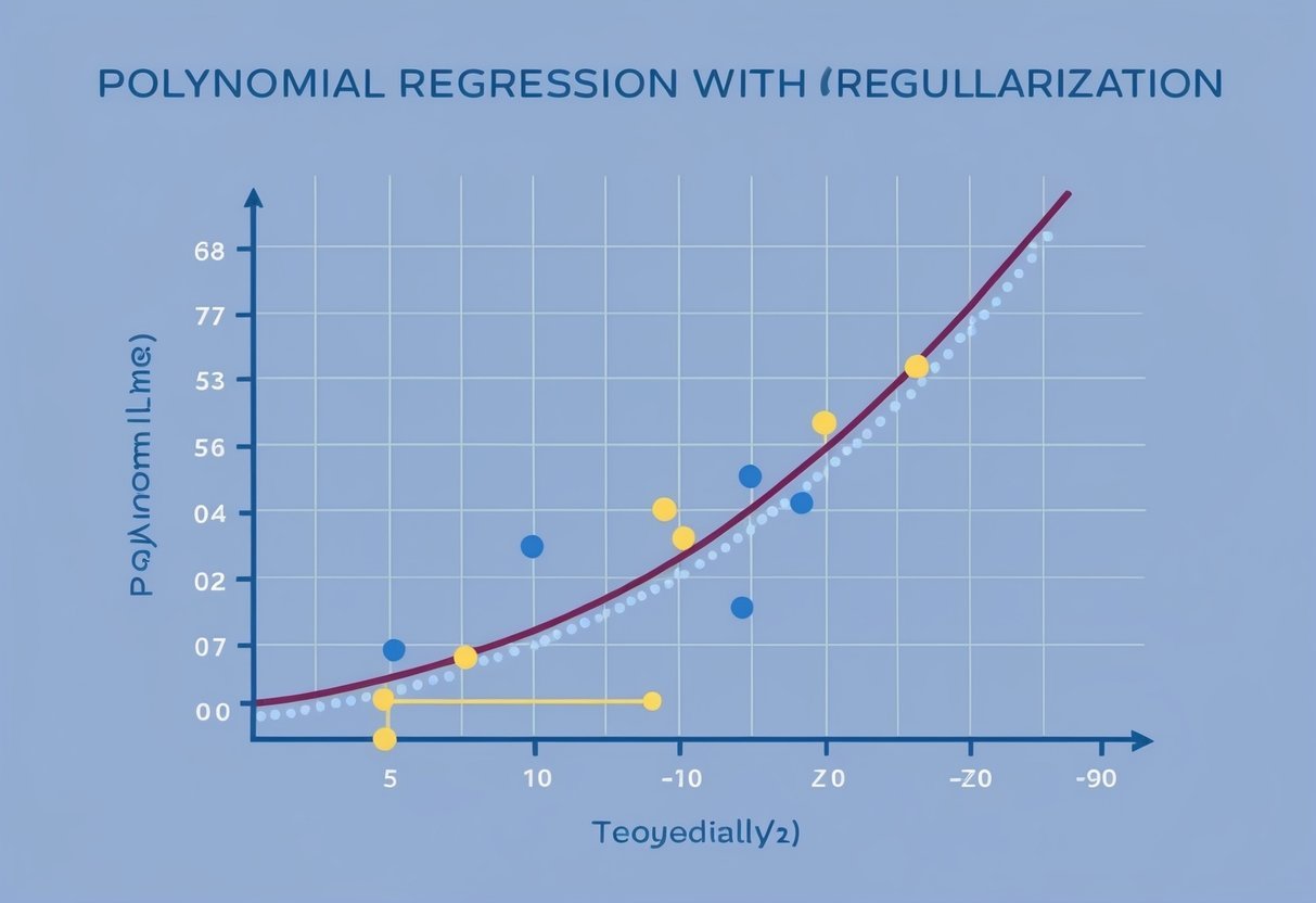
Graphs of polynomial fits highlight how model complexity affects overfitting. As the degree increases, the fit becomes wavier, adjusting to every detail in the training data.
At higher polynomial degrees, the risk of overfitting increases, emphasizing the need for techniques like cross-validation to ensure the model performs well on unseen data.
Regularization Techniques in Regression
Regularization in regression involves techniques that add a penalty term to prevent overfitting. This helps in managing model complexity by discouraging overly complex models that may not generalize well to new data. The main techniques include Ridge Regression, Lasso Regression, and Elastic Net Regression.
Ridge Regression Explained
Ridge Regression, also known as L2 regularization, is a technique that adds a penalty term proportional to the square of the coefficients’ magnitude. This method is beneficial in scenarios with multicollinearity where features are highly correlated.
By shrinking the coefficients, it ensures no feature dominates the model, enhancing prediction accuracy.
Ridge Regression is particularly useful for models with many variables, as it helps maintain stability.
Moreover, it is effective where datasets have more predictors than observations. This makes it a robust choice for high-dimensional data.
The penalty term, represented as lambda (λ), controls the strength of the regularization, and tuning this parameter is crucial for optimal performance.
Lasso Regression and Its Characteristics
Lasso Regression stands for Least Absolute Shrinkage and Selection Operator and is an example of L1 regularization. Unlike Ridge, Lasso can reduce some coefficients to zero, effectively selecting a simpler model.
This characteristic makes it ideal for feature selection, as it simultaneously performs shrinkage and variable selection.
By promoting sparsity, Lasso helps identify the most important predictors in a dataset. It excels in situations where only a few features carry significant predictive power, ensuring the model remains interpretable.
However, Lasso might struggle with datasets where variables are highly correlated, as it might arbitrarily assign significance to one feature over another. Therefore, careful consideration is needed when applying it to such data.
Understanding Elastic Net Regression
Elastic Net Regression combines both L1 and L2 regularizations. It addresses the limitations of Ridge and Lasso by adding both kinds of penalty terms to the model.
This hybrid approach is particularly effective in datasets with correlated variables, where both Ridge and Lasso individually might fall short.
Elastic Net is versatile, allowing for variable selection and handling multicollinearity effectively. It uses two parameters to control the penalty terms, offering greater flexibility.
The mixing parameter determines the balance between L1 and L2 penalties, providing a nuanced control over the level of regularization applied.
By leveraging the strengths of both Ridge and Lasso, Elastic Net is suitable for complex datasets requiring a delicate balance between feature selection and coefficient shrinkage.
Preparing Data for Polynomial Regression
When preparing data for polynomial regression, two critical steps are feature engineering and data scaling. These steps ensure that the model captures complex patterns accurately and performs well across various datasets.
Feature Engineering with PolynomialFeatures
Feature engineering involves creating new input features that can aid in modeling non-linear relationships. In polynomial regression, this is achieved using the PolynomialFeatures class from libraries like scikit-learn.
This class transforms the original features into a design matrix that includes polynomial terms up to the desired degree. By leveraging these polynomial terms, models can effectively capture the curvature in the data.
Creating a comprehensive set of polynomial features is crucial. It allows the model to fit complex data patterns, potentially reducing training error.
These features can be adjusted by choosing the degree of the polynomial, which should be determined based on the specifics of the dataset. Excessively high degrees might lead to overfitting, where the model performs well on the training data but poorly on new data.
Importance of Data Scaling
Data scaling plays a vital role in polynomial regression. Using techniques like StandardScaler, one can standardize features by removing the mean and scaling to unit variance.
This process is essential, especially when dealing with polynomial features, as it ensures that all features contribute equally to the model’s outcome.
Without proper scaling, features with larger ranges might disproportionately influence the model, resulting in biased predictions.
Standardization helps in improving the convergence of optimization algorithms used in training the model. It is particularly important when implementing regularization techniques that add penalty terms to reduce the risk of overfitting.
Properly scaled data enhances the stability and effectiveness of polynomial regression models, ensuring that they perform consistently across different datasets.
Optimizing Polynomial Models with Hyperparameters
Optimizing polynomial models involves selecting the right polynomial degree and applying regularization to prevent overfitting. Proper tuning of hyperparameters ensures that the model captures the data pattern effectively and generalizes well to new data.
Choosing the Degree of Polynomial
Selecting the degree of the polynomial is crucial for model performance. A polynomial degree that’s too low might fail to capture complex data patterns, while a degree that’s too high can lead to overfitting. The degree is a key hyperparameter that dictates the shape and complexity of the polynomial function.
Using techniques like cross-validation can help in choosing the ideal degree. This involves dividing the data into training and validation sets and evaluating model performance for different polynomial degrees.
Cross-validation provides a reliable performance estimate on unseen data. Automated tools such as grid search can also assist by testing multiple degree values systematically.
Finding the balance between underfitting and overfitting is essential. A well-chosen degree should provide an accurate fit without excessive complexity.
Applying Regularization Hyperparameters
Regularization addresses overfitting by introducing additional terms to the loss function. In polynomial regression, regularization hyperparameters, such as L1 and L2, play a vital role in controlling model complexity.
L1 regularization, or Lasso, adds the absolute values of the coefficients to the loss function, encouraging sparsity in model weights.
This can be useful when feature selection is needed.
L2 regularization, or Ridge, involves adding the squared values of coefficients, helping to reduce sensitivity to small fluctuations in the training data.
Tuning regularization parameters involves adjusting the strength of these penalties to achieve a balance between bias and variance. Automated searches, like grid search or random search, can efficiently explore different values.
This step ensures that the model’s predictions remain stable and reliable, even with more complex polynomial degrees.
Setting Up Regression Models in Python
Setting up regression models in Python often involves using libraries like scikit-learn. This section will explore how to utilize scikit-learn for creating robust models and apply Python code to polynomial regression scenarios effectively.
Utilizing the scikit-learn Library
Scikit-learn is a powerful Python library used for machine learning. It provides tools for data analysis and model building.
One important aspect of setting up regression models is the preparation and transformation of data, which can be easily achieved with scikit-learn’s preprocessing features.
To get started, users import the necessary modules. For polynomial regression, data must be transformed to include polynomial features. This is handled using the PolynomialFeatures class.
By choosing the degree of the polynomial, users can tailor the complexity of the model. After setting up the features, fit the model using LinearRegression.
Creating models with scikit-learn is made more efficient due to its simple and consistent API. It allows users to implement and experiment with different model parameters swiftly, which is crucial for developing effective machine learning models.
Using scikit-learn simplifies integrating gradient descent, enabling optimization of weights during training.
Applying Python Code to Polynomial Regression
In Python, applying code to implement polynomial regression involves several steps.
First, data needs to be arranged, typically in a NumPy array. This array becomes the foundation for constructing the regression model.
Once data is structured, the PolynomialFeatures transformer is applied to increase the dimensionality of the dataset based on the desired polynomial degree. After that, the transformed data feeds into a LinearRegression model.
The model learns by applying algorithms like gradient descent, which helps minimize the error by adjusting weights. This process can be iteratively refined to enhance accuracy.
Practical application of polynomial regression through Python code requires a balance between fitting the data well and avoiding overfitting, often tackled by validating the model using cross-validation methods to ensure its performance on various data samples.
Analyzing Model Fit and Predictions

To understand the effectiveness of a polynomial regression model, it is crucial to evaluate how well the model fits the data and makes predictions. Key aspects include examining coefficients and intercepts, as well as precision and recall metrics.
Interpreting the Coefficients and Intercept
In polynomial regression, the coefficients play a vital role in shaping the model’s behavior. Each coefficient corresponds to the degree of the variable in the equation, contributing uniquely to the model’s output.
Specifically, the intercept represents the value of the dependent variable when all predictors are zero.
Understanding these components helps assess model fit. Large coefficients might indicate the model is too sensitive to specific data points, potentially leading to overfitting.
Proper analysis of coefficients helps in tweaking the model to achieve optimal balance between bias and variance.
Understanding Precision and Recall
Evaluating precision and recall is essential when analyzing the predictive performance of the model. Precision measures the accuracy of predictions labeled as positive, while recall reflects the model’s ability to identify all relevant instances in the dataset.
High precision means fewer false positives, and high recall indicates fewer false negatives.
Balancing precision and recall ensures reliable predictions, reducing the chances of error. By refining these metrics, users can fine-tune their models to better meet specific analytical goals in polynomial regression.
Loss Functions and Model Evaluation
In polynomial regression, evaluating the model’s effectiveness is crucial. Key metrics like the mean squared error (MSE) help provide insights into model performance.
These metrics guide the selection and tuning of models to achieve optimal results.
Role of Mean Squared Error in Regression
The mean squared error (MSE) is an important metric to assess a model’s accuracy. It measures the average of the squares of the errors, which are the differences between the predicted and actual values.
A smaller MSE indicates a model that fits the data well, providing valuable insights into model performance.
MSE can be calculated using this formula:
[
text{MSE} = frac{1}{n} sum_{i=1}^n (y_i – hat{y_i})^2
]
where (y_i) is the actual value and (hat{y_i}) is the predicted value.
Lower MSE values reflect a more accurate model. It is widely used because it penalizes larger errors more harshly than smaller ones.
Considering Training Loss in Model Selection
Training loss is a key factor during the model selection process. It refers to the error calculated on the training dataset using a loss function.
Common loss functions in regression include MSE and absolute error. Lower training loss suggests that the model is well-tuned to the training data, indicating good initial performance.
However, selecting a model solely based on training loss can be misleading if not compared with validation loss.
Overfitting can occur if the model performs well on training data but poorly on unseen data. Thus, monitoring both training and validation losses ensures robust model evaluation and selection.
Most techniques balance these aspects to prevent overfitting and boost generalization capabilities.
Understanding Model Generalization
Model generalization is the ability of a machine learning model to perform well on unseen data, beyond its training set. It ensures that the model is not just memorizing the training data but can also handle new, unknown inputs effectively.
Strategies to Improve Model Generalization
One of the key strategies to improve generalization is regularization. This involves adding a penalty to the loss function to reduce model complexity.
Techniques such as Ridge and Lasso regression prevent overfitting by discouraging large coefficients. These methods adjust the model to become simpler and more robust when facing new data, ultimately enhancing its generalization capabilities.
Another effective approach is to use cross-validation for model evaluation. By splitting the data into multiple sets for training and testing, cross-validation provides a more accurate estimate of model performance.
This helps in diagnosing overfitting and underfitting. Utilizing cross-validation ensures that the model’s ability to generalize is thoroughly assessed before deployment.
Through this, models become more reliable in practical applications.
Managing Non-Linear And Polynomial Relationships
Polynomials can capture complex patterns in non-linear data, which linear models fail to do. This is achieved by transforming features and using polynomial models to reveal hidden trends and relationships.
Detecting Non-Linear Patterns
In data analysis, it is crucial to identify when data relationships are non-linear. Linear relationships have a constant rate of change, but non-linear relationships do not.
They can be spotted by graphing data points and looking for curves or bends, instead of straight lines. When non-linear patterns are present, polynomial regression becomes useful.
Polynomial models allow for curves and bends by using polynomial equations, such as quadratic or cubic forms. This provides flexible fitting of non-linear relationships.
By comparing different polynomial models—quadratic, cubic, etc.—the best fit for the data can be chosen. This selection helps enhance prediction accuracy, adapting to the curvature seen in the data.
Linear Models as a Subset of Polynomial Regression
Polynomial regression is a method used to model the relationship between a dependent variable and independent variables as an nth degree polynomial. It offers a broader scope compared to linear models. This is because linear models are a specific case of polynomial regression where the polynomial degree is one.
In simple linear regression, the model equation is typically formatted as y = a + bx, with a and b representing the coefficients, and x representing the independent variable. This type of model only captures linear relationships.
Simple Linear Regression vs. Polynomial Regression:
| Model Type | Equation | Characteristics |
|---|---|---|
| Simple Linear | y = a + bx | Predicts a straight line |
| Polynomial (Degree 2) | y = a + bx + cx² | Captures curves (quadratic) |
| Polynomial (Degree 3) | y = a + bx + cx² + dx³ | Models more complex patterns (cubic) |
Polynomial regression extends this by including squares, cubes, and higher powers of the variable, allowing the model to fit more complex data patterns.
While simple linear regression works well for straightforward linear relationships, polynomial regression is valuable when the data shows curvature. For instance, if data points form a parabola, a quadratic polynomial model (degree 2) might be ideal.
You can see more about the usefulness of such models by checking training models: polynomial regression.
This approach combines the simplicity of linear models while offering flexibility to adapt to non-linear trends. Thus, linear models can be seen as the simplest form of polynomial regression, providing a good starting point for statistical analysis.
Frequently Asked Questions
This section covers important aspects of polynomial regression, including its implementation in Python, real-world uses, and formal notation. It also explores determining the optimal polynomial degree and setting up data with regularization.
How do you implement polynomial regression regularization in Python?
Polynomial regression with regularization in Python can be implemented using libraries like scikit-learn.
Tools such as PolynomialFeatures transform input data, while Ridge or Lasso from sklearn.linear_model apply regularization, reducing overfitting by penalizing large coefficients.
What are some real-life examples of polynomial regression applications?
Real-life applications of polynomial regression include predicting population growth, modeling financial trends, and analyzing the relationship between power output and engine size.
These applications demonstrate how polynomial models can capture non-linear patterns in complex datasets.
What is the formal notation used for expressing a polynomial regression model?
A polynomial regression model is often expressed as ( y = beta_0 + beta_1x + beta_2x^2 + ldots + beta_nx^n + epsilon ), where ( y ) is the output, ( x ) is the input variable, (beta)s are the coefficients, ( n ) is the degree, and ( epsilon ) is the error term.
How can you determine the optimal degree of a polynomial in regression analysis?
Determining the optimal degree of a polynomial involves balancing model complexity and fitting accuracy.
Techniques such as cross-validation or using a validation set can help assess different polynomial degrees and select the one that minimizes prediction error while avoiding overfitting.
What is the process for setting up data for polynomial regression with regularization?
To set up data for polynomial regression with regularization, start by transforming your features using PolynomialFeatures.
Next, split the data into training and test sets, apply a regularization technique like Ridge or Lasso, and train the model to reduce overfitting risks.
In Python, how can the degree of a polynomial be set using PolynomialFeatures?
In Python, the degree of a polynomial is set using PolynomialFeatures from sklearn.preprocessing.
By specifying the degree parameter, users can define the highest power of the polynomial, allowing the model to capture varying degrees of data complexity based on requirements.