Learning about Polynomial Regression – Cross Validation Techniques Explained

Understanding Polynomial Regression

Polynomial regression is a type of regression analysis. It models the relationship between the independent variable (x) and the dependent variable (y) as an (n)th degree polynomial.

Key Components

Coefficients: These are the parameters of the polynomial model. They determine the shape and position of the polynomial curve.
Vandermonde Matrix: This matrix is used to set up the polynomial regression problem. It enables the transformation of input data into a format that fits a polynomial equation.
Least Squares Method: This method helps in finding the coefficients that minimize the error between the predicted and actual observations. It measures errors as the sum of squared differences.

Noise and Observations

When real-world data is studied, the presence of noise is inevitable.

Noise refers to random errors or fluctuations in the observed data. It can affect the accuracy of polynomial regression by making it harder to detect the true pattern.
Noisy Observations are dataset entries with a high degree of noise. They can disturb the model’s accuracy by making it fit the noise rather than the underlying trend.

Uses and Applications

Polynomial regression is widely used in various fields, such as engineering and finance, to model non-linear relationships.

It can capture complex patterns in data while maintaining flexibility to accommodate different data structures.

By selecting the appropriate degree and managing noise, polynomial regression can provide insights into data that linear models might miss.

Fundamentals of Regression Analysis

Regression analysis is a powerful tool used to identify the relationships between variables. It is widely applied in predicting outcomes and assessing trends based on data.

Key concepts include differentiating between linear and polynomial approaches, understanding the role of coefficients, and fitting a regression model using techniques like least squares.

Linear vs Polynomial Regression

Linear regression is the simplest form, focusing on a straight-line relationship between the dependent and independent variables.

It uses the equation ( Y = beta_0 + beta_1X ), where (beta_0) and (beta_1) are the intercept and slope, respectively. This approach works well when the relationship looks like a straight line.

Polynomial regression extends linear regression to identify more complex, nonlinear relationships.

It fits data to a polynomial equation such as ( Y = beta_0 + beta_1X + beta_2X^2 + ldots + beta_nX^n ). This is useful in predicting trends where data points curve significantly.

Both types of regression have their uses and limitations. Choosing the right type depends on the data pattern.

Linear regression is preferred for simplicity and fewer computations, while polynomial regression can model more complex patterns but may risk overfitting if not carefully managed.

The Role of Coefficients

Coefficients in a regression model are crucial as they represent the strength and direction of the relationship between variables.

In linear regression, for instance, the slope coefficient shows how much the dependent variable changes with a unit change in the independent variable. A positive slope suggests a positive association while a negative slope indicates the opposite.

In polynomial regression, coefficients are critical in shaping the curve of the regression line. Each coefficient has a specific role, impacting the curve’s steepness, direction, and the overall fit of the model.

Higher-degree polynomials can provide a better fit but also increase the complexity.

Fitting the Regression Model

Fitting a regression model involves finding the best line or curve that minimizes the difference between actual data points and predicted values.

The least squares method is often employed for this purpose. It calculates the sum of the squares of the residuals, which are the differences between observed and predicted values, and seeks to minimize this sum.

In practice, the process involves iterative adjustments to the coefficients to find the values that offer the best fit.

Software tools and frameworks like scikit-learn offer efficient ways to perform this fitting by providing functions to automate the process.

Challenges in fitting the model include ensuring it does not overfit or underfit the data.

Rather than following a one-size-fits-all approach, it is essential to evaluate each model’s performance using relevant metrics.

Overview of Cross Validation Techniques

Cross-validation is a key technique in evaluating the effectiveness of machine learning models. It helps in assessing how well a model will perform on unseen data.

By understanding and applying different methods, one can improve model selection processes and enhance predictive accuracy.

Purpose of Cross-Validation

Cross-validation aims to provide a more reliable estimate of a model’s performance. It addresses the issue of overfitting by using different subsets of the data for training and testing.

This method ensures that every data point has the opportunity to be in both the training and testing set.

Cross-validation helps in making sure that the model learns the underlying patterns rather than memorizing the data. This enhances the model’s ability to generalize to new data effectively, providing an accurate picture of its predictive power.

Distribution of data points across various splits mitigates bias and improves model reliability.

Types of Cross-Validation

There are several types of cross-validation, each with its strengths.

K-fold cross-validation is common and involves breaking data into k distinct subsets or folds. The model is trained and tested k times, each time using a different fold as the test set and others as the training set.

Hold-out cross-validation divides the dataset into two parts: training and testing. While it’s simpler, it may not utilize all data points for both testing and training, which can lead to bias if the split isn’t representative.

Understanding these variations helps in choosing the most suitable method for different datasets and model complexities, optimizing the performance efficiently.

Dealing with Overfitting in Polynomial Regression

Overfitting is a common problem in polynomial regression. It occurs when a model is too complex and captures the noise in the data rather than the actual patterns. This often results in misleading coefficients and poor predictions on new data.

To address overfitting, one can use cross-validation techniques.

Cross-validation involves splitting the dataset into training and validation sets. The model is trained on one set and tested on the other to ensure it performs well on unseen data. This helps in choosing the appropriate complexity for the model.

Another way to detect overfitting is by examining the Mean Squared Error (MSE).

A model with a very low MSE on the training data but a high MSE on validation data is likely overfitting. By comparing these errors, one can adjust the polynomial degree for a better fit.

Regularization is also an effective method to combat overfitting.

Techniques like Lasso or Ridge regression add a penalty to the size of the coefficients. This prevents the model from becoming too complex and minimizes the effect of noise.

Selecting the right polynomial degree is crucial.

Tools like cross-validation help in identifying the best degree to reduce overfitting.

It’s important to balance bias and variance to achieve a reliable regression model that generalizes well to new data.

Selecting the Degree of the Polynomial

When choosing the degree for a polynomial regression model, it is important to consider both the model’s ability to fit the data and its complexity. Striking the right balance is key to achieving strong predictive performance without overfitting.

Implications of Polynomial Degree

The degree of a polynomial significantly affects the shape and flexibility of the model. A higher degree allows the model to fit the data more closely, which can reduce training error but may also lead to overfitting.

Overfitting happens when the model learns noise in the data rather than the underlying pattern, resulting in poor performance on new data.

An optimal degree balances complexity and fit. Choosing too low a degree might result in underfitting, where the model is too simple to capture important patterns.

Experimentation and domain knowledge can guide the selection of a degree suitable for the dataset and the problem at hand.

Evaluating Model Complexity

Model complexity can be evaluated using methods like cross-validation, which involves splitting the dataset into training and validation sets.

By calculating metrics such as validation error or RMSE (Root Mean Squared Error) for different degrees as suggested by discussions on Stack Overflow, one can identify the degree that offers the best predictive performance.

When the validation error stops decreasing significantly, or starts increasing as the degree increases, the degree can be considered optimal.

K-fold cross-validation is a robust approach where the data is divided into k parts, and the model is trained and validated k times, each time using a different partition of the data. This provides a thorough assessment of how the model is likely to perform in practice.

Evaluating Regression Models

Assessing regression models involves understanding key performance metrics and interpreting various errors, such as training and validation errors. These insights are crucial for improving model accuracy and generalization.

Metrics for Performance Evaluation

Predictive accuracy is vital in evaluating regression models. It helps in determining how well a model makes predictions on new, unseen data.

Common metrics include Mean Squared Error (MSE) and R-squared.

MSE measures the average squared difference between actual and predicted values, indicating how close predictions are to actual data points.

R-squared examines the proportion of variance in the dependent variable explained by the model. This metric shows how well the model fits the data.

Cross-validation is another important tool that aids in estimating a model’s performance.

By splitting data into training and test sets multiple times, it evaluates a model’s ability to generalize. This technique minimizes overfitting, ensuring that the model performs well on diverse datasets.

Interpreting Validation Errors

Validation errors assess a model’s performance on unseen data.

Training error is the error the model makes on the training set, while validation error reveals how well the model predicts on a separate set. A significant discrepancy between these can indicate overfitting.

Cross-validation error helps detect overfitting by evaluating the model’s performance across different data folds.

Generalization error reflects the model’s performance on entirely new data. Lower generalization errors signify better accuracy on new inputs. Lastly, empirical error is observed through testing, helping to refine the model by reducing discrepancies between predicted and actual outcomes.

Practical Implementation with Scikit-Learn

Implementing polynomial regression using Scikit-Learn involves techniques such as Polyfit for fitting polynomials and GridSearchCV for hyperparameter tuning. Integrating these methods with pipelines and estimators can enhance machine learning workflows efficiently.

Utilizing Polyfit and GridSearchCV

Scikit-Learn can interact seamlessly with NumPy to fit polynomial curves. The function np.polyfit is commonly used to fit a polynomial of a specified degree to data. This allows the creation of a model that captures nonlinear patterns in the data.

Although Polyfit is a NumPy tool, Scikit-Learn’s GridSearchCV complements it by optimizing hyperparameters of the polynomial model.

Table: Key Functions

Function	Description
`np.polyfit`	Fits polynomials to data points
`GridSearchCV`	Optimizes model hyperparameters using cross-validation

Combining these allows users to find the best polynomial degree and refine model parameters. This approach ensures the model fits the data well without overfitting.

Pipeline Integration with Estimators

Scikit-Learn’s pipeline feature is invaluable for building complex models. Pipelines allow users to chain together a sequence of transformations and estimators, streamlining the workflow.

When integrating polynomial regression, estimators such as PolynomialFeatures transform the input features into polynomial terms.

Steps to Implement:

Create Transformer: Use PolynomialFeatures to transform data.
Build Pipeline: Combine PolynomialFeatures with a regression estimator like LinearRegression.
Fit Model: Use the pipeline to fit data. This automates transformations and fitting.

Using pipelines simplifies the process and reduces errors by encapsulating the entire workflow. This integration improves the consistency and reliability of polynomial regression models in machine learning applications.

Preparing Your Dataset for Training

Preparing a dataset is crucial for building a reliable model.

Key tasks include splitting data into training and test sets, and ensuring the quality of the data used for training to avoid any bias or inaccuracies in results.

Splitting Data into Training and Test Sets

Splitting a dataset into distinct parts is important to evaluate how the model performs. Typically, data is divided into a training set and a test set.

The training set is used to train the model, while the test set evaluates its performance. A common method for this is the train_test_split function, which efficiently splits the data.

Using a standard practice, the data might be divided in an 80-20 ratio, where 80% is used for training, and 20% is for testing. This ensures the model is tested on data it hasn’t seen before, helping to assess its predictive power. This process is also known as creating a holdout set, as mentioned in the concept of the holdout method.

Ensuring Data Quality for Training

Data quality is vital for effective model training. Before using data to train a model, it should be cleaned and preprocessed to remove any inconsistencies or errors.

This includes handling missing values, correcting inaccurate entries, and ensuring data is normalized or standardized if needed.

Ensuring the consistency and relevance of the data prevents biases and errors. For instance, all features should be in the correct format, and skewed data should be adjusted.

Consistent formatting helps the algorithm learn patterns accurately, leading to better prediction outcomes. Detecting and handling outliers is also necessary to avoid skewed results, ensuring that the models built on the training set are robust and reliable.

Weight Adjustment and Learning Rules

Adjusting weights in polynomial regression involves applying specific learning rules and optimization techniques. These methods ensure that the model accurately predicts outcomes by minimizing the error through refined adjustments.

Understanding the Delta Learning Rule

The delta learning rule is a fundamental approach for adjusting weights in machine learning models. It focuses on minimizing the difference between actual and predicted values.

The rule updates the weight by a small amount based on the error observed in each iteration.

This adjustment is calculated as the product of the learning rate and the gradient of the error concerning the weight. By iteratively adjusting the weights, the algorithm refines the model’s accuracy.

The learning rate determines the size of each step towards error minimization. A balanced learning rate is crucial; a rate too high can overshoot the minimum error, while a rate too low can make the process too slow.

Weight Optimization Techniques

Several techniques aim to optimize the weights efficiently.

Gradient Descent is a popular method, where the model iteratively moves towards the lowest point on the error surface.

Variants like Stochastic Gradient Descent (SGD) reduce computation time by updating weights based on a single data point rather than the whole dataset.

Other methods, such as Adam and RMSprop, adjust learning rates dynamically during training, which can lead to faster convergence.

These techniques help balance speed and accuracy, crucial for effective model training. Employing these will improve model performance by efficiently finding the optimal weights. Adjustments are made systematically to reach the minimal error possible, ensuring reliable predictions.

Assessing Model Confidence and Intervals

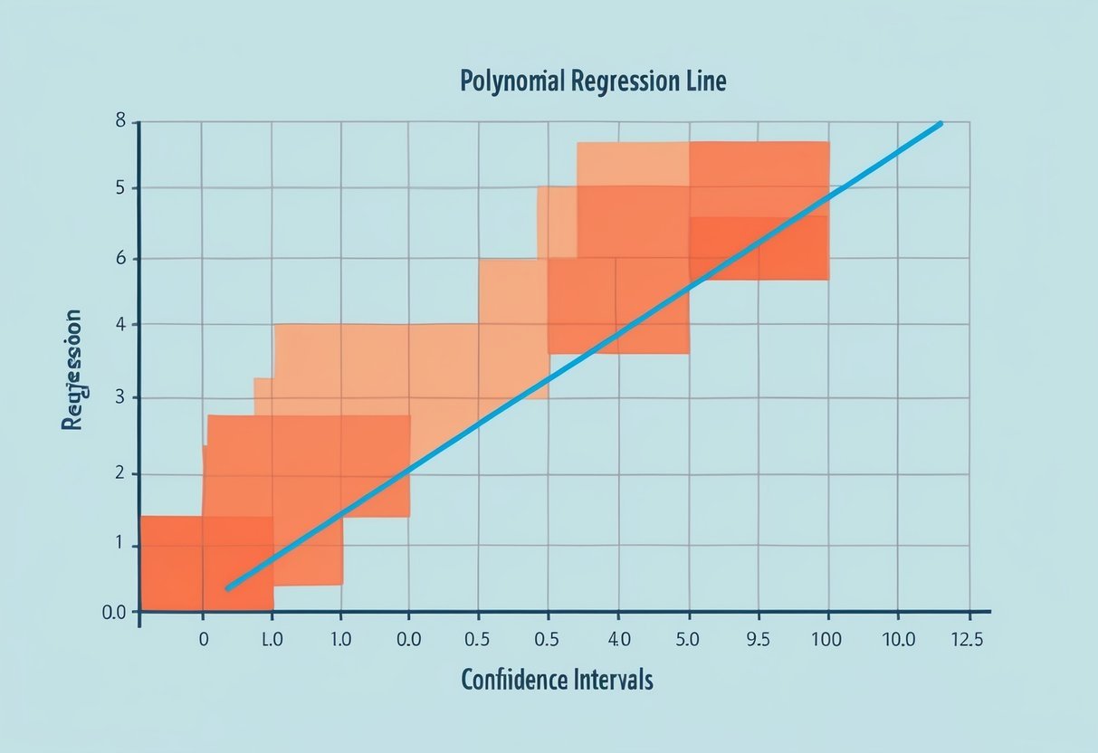
When evaluating a polynomial regression model, it’s important to consider confidence intervals. These intervals provide a range of estimates for where the true regression coefficients lie.

Confidence intervals help identify the reliability of the predictions.

The degree of the polynomial affects the model’s predictive performance. A higher-degree polynomial might fit the training data well but may perform poorly on new data due to overfitting. Cross-validation can be used to select the appropriate degree, balancing complexity and accuracy.

Confidence Intervals Table:

Degree of Polynomial	Confidence Interval Width	Predictive Performance
1	Narrow	Moderate
2	Moderate	Improved
3+	Wide	Risk of Overfitting

This table suggests that as the degree increases, the confidence interval width often increases, indicating potential overfitting. Narrow intervals suggest that the model is stable and reliable.

Assessing model confidence also involves checking how predictions vary with input changes. Smaller predictive errors within the confidence intervals indicate that the model generalizes well.

By using cross-validation along with confidence intervals, one can ensure that the chosen polynomial degree provides a balance between fit and predictive accuracy. This method is critical for making informed decisions regarding the reliability of the regression model.

Frequently Asked Questions

Polynomial regression and cross-validation often go hand in hand in building robust models. Key aspects include how cross-validation is conducted, its importance in evaluating models, and differences from other regression types.

How is cross-validation performed in polynomial regression?

Cross-validation in polynomial regression involves dividing data into parts, or folds. Models are trained on part of the data and validated on the remaining part. This helps estimate how well a model will perform on unseen data.

What are the steps to implement polynomial regression in Python with cross-validation?

To implement polynomial regression with cross-validation in Python, one can use libraries like scikit-learn. The steps typically include creating polynomial features, splitting the dataset, choosing a cross-validation strategy, and training the model to evaluate its performance.

Can you explain the role of K-fold cross-validation in assessing polynomial regression models?

K-fold cross-validation helps ensure a model’s reliability by using different subsets of data for training and validation. By rotating through different partitions, it provides a comprehensive assessment of how well the polynomial regression model can generalize.

What are some common examples where polynomial regression is an appropriate model to use?

Polynomial regression is useful when data shows a curvilinear relationship. Examples include growth rate analysis and trends in data that do not follow a straight line, such as predicting population growth or analyzing certain economic metrics.

How does polynomial regression differ from multiple linear regression?

Polynomial regression uses higher-degree polynomials to capture nonlinear relationships in the data, unlike multiple linear regression, which assumes a straight-line relationship among variables. This makes polynomial regression suitable for more complex data patterns.

Why is cross-validation crucial for evaluating the performance of a regression model?

Cross-validation is vital for checking how a regression model will perform on new data. It helps prevent overfitting by ensuring that the model captures the underlying data pattern without memorizing the noise or specific details.