
Understanding Polynomial Regression
Polynomial regression is a technique used to model nonlinear relationships between variables. It extends linear regression by introducing polynomial terms, allowing for the modeling of curves.
In polynomial regression, the model takes the form:
[ y = beta_0 + beta_1x + beta_2x^2 + … + beta_nx^n + epsilon ]
Key Components:
- Dependent Variable (y): The outcome or response variable.
- Independent Variable (x): The predictor variable.
- Coefficients ((beta)): Values that adjust the shape of the curve.
While linear regression is suitable for straight-line relationships, polynomial regression is used for data with curves. By increasing the degree of the polynomial, the model can fit more complex patterns.
Applications in Machine Learning:
Polynomial regression is essential in machine learning for capturing non-linear patterns. It can handle situations where linear models fail. However, it’s crucial to avoid overfitting by using appropriate polynomial degrees.
Comparison with Linear Regression:
- Linear Regression: Takes the form ( y = beta_0 + beta_1x ).
- Polynomial Regression: Includes higher-order terms for flexibility.
This method is widely used in fields such as economics and biology, where data often exhibit curvilinear trends. For a more detailed explanation, consider reading about polynomial regression models. These models are integral in understanding complex data structures.
Exploring the Fundamentals of Polynomial Features
Polynomial features play a crucial role in enhancing regression models by capturing more complex relationships in data. They transform original input variables into a richer set of features, allowing models to fit non-linear patterns more effectively.
The Role of Polynomial Terms
Polynomial terms are essentially new features created by raising existing features to a specified power. These terms help in modeling non-linear relationships.
By including polynomial terms, a model can better fit curves and interactions between features that linear models might miss.
Using polynomial terms allows the model to account for interactions between features. For instance, if two features influence each other, polynomial terms can capture this interaction, offering a more comprehensive view of the data.
Difference Between Linear and Polynomial Models
Linear models are limited to relationships that form straight lines, meaning they assume a constant rate of change. This is a limitation when working with non-linear data sets where relationships are more complex.
In contrast, polynomial models expand the capabilities by creating additional features. These models can fit curves and bends, better capturing the actual patterns in the data.
This flexibility is essential for datasets with more complex interactions between features, setting polynomial models apart from their linear counterparts.
Setting Up the Regression Environment
Polynomial regression requires specific tools and careful data preparation. Knowing which libraries to use and how to pre-process your data is key to building a successful model.
This section explores the essential libraries for performing polynomial regression and outlines steps to get your data ready for modeling.
Tools and Libraries for Polynomial Regression
Python is an ideal choice for polynomial regression, offering a variety of libraries to simplify the process.
NumPy and Pandas are fundamental, providing data structures and mathematical functions essential for handling and manipulating data.
Scikit-learn is a powerful library widely used for polynomial regression. It includes tools such as PolynomialFeatures from the sklearn module, which transforms input data by adding polynomial terms.
Using Scikit-learn, users can easily build, train, and evaluate models. The library offers functions for splitting data into training and test sets, fitting models, and evaluating accuracy.
These tools streamline the workflow and reduce the effort needed to implement complex algorithms. With these libraries, users have a comprehensive set of tools to tackle polynomial regression problems efficiently.
Preparing Your Data for Modeling
Data preparation is crucial and involves several steps.
First, data should be cleaned and formatted correctly, using Pandas for tasks like handling missing values and standardizing format. This ensures data quality and consistency.
Next, data transformation is necessary, especially when dealing with polynomial regression.
Implementing PolynomialFeatures from Scikit-learn helps in converting linear data into polynomial format by creating interaction and power terms. This step is essential for capturing the complexity of data relationships.
Lastly, splitting the dataset into training and testing sets is vital for model evaluation. Scikit-learn offers convenient methods like train_test_split to streamline this process.
By correctly setting up the environment, the accuracy and reliability of the polynomial regression model are greatly enhanced.
Designing Polynomial Regression Models
Designing polynomial regression models involves selecting the right degree and applying feature transformation techniques to capture non-linear relationships. These steps help to tailor the model for better predictive power without overfitting the data.
Choosing the Degree of Polynomial
Determining the degree of polynomial is crucial for model flexibility. A low degree may not capture the complexity of the data, while a high degree can lead to overfitting.
In simple linear regression, the relationship is modeled with a straight line. In contrast, polynomial linear regression uses curves to fit the data, allowing the model to adapt more closely to the nuances in the dataset.
The selection process often involves testing multiple polynomial degrees to find the sweet spot where the model predicts accurately without memorizing training data.
Analysts can use cross-validation techniques to compare performance across varied degrees and select an optimal one, balancing bias and variance effectively.
Feature Transformation Techniques
Feature transformation plays a key role in building a robust regression model. By transforming input features, models can better capture underlying patterns.
This involves raising input variables to power levels defined by the chosen polynomial degree, effectively increasing the model’s ability to capture complex relationships.
Polynomial linear regression does not modify the basic assumption that the relationship is linear in terms of coefficients, but it transforms features to include powers of variables. This method makes it possible for the model to fit non-linear data patterns.
Proper feature transformation helps in maintaining model accuracy while avoiding overfitting, providing a balance between complexity and predictive performance.
Training and Testing the Model
Training and testing a model are essential steps in supervised learning, ensuring that a model can make accurate predictions on new data. It involves creating separate datasets, one for training and one for testing the model’s performance.
Creating the Training and Testing Datasets
In supervised learning, data is divided into two main parts: a training set and a testing set. The training set is used to teach the model how to understand the data by adjusting its parameters based on this input.
Typically, about 70-80% of the data is allocated to the training set, although this can vary depending on the size of the dataset.
The remaining data becomes the testing set. This testing data is crucial because it evaluates how well the model performs on unseen data, providing an estimate of its prediction accuracy.
The division of data ensures that the model doesn’t simply memorize the training data but can also generalize to new inputs. This avoids issues like overfitting, where a model performs well on training data but poorly on testing data.
The Process of Model Training
Model training is the process where the training data is used to adjust a model’s parameters.
In the context of polynomial regression, coefficients of polynomials are adjusted to minimize the difference between the predicted and actual values in the training set. This process relies on optimization algorithms that find the best fit for the data.
Training involves multiple iterations, where the model learns progressively better representations of the data structure. Each iteration adjusts the coefficients to reduce errors, improving the model’s ability to capture the underlying patterns of the training data.
This process equips the model with the capacity to make accurate predictions for the testing data, ideally achieving a balance between accuracy and complexity.
Performance Metrics for Polynomial Regression
Performance metrics help to evaluate how well a polynomial regression model fits the data. Two key metrics are Mean Squared Error (MSE) and R-squared. These metrics assist in understanding the model’s performance and accuracy by quantifying prediction errors and the proportion of variance explained by the model.
Understanding Mean Squared Error
Mean Squared Error (MSE) is a widely used metric to measure accuracy in polynomial regression. It calculates the average of the squares of the errors, where error is the difference between the observed and predicted values.
A lower MSE indicates better model performance, as it shows that the predictions are closer to true values.
MSE is useful as it penalizes large errors more than small ones, providing a clear insight into the model’s precision. This makes it a preferred choice when the goal is to minimize errors in predicting outcomes.
By focusing on squared differences, MSE can guide adjustments to model parameters to improve accuracy.
Interpreting the R-Squared Value
R-squared, also known as the coefficient of determination, measures how much variance in the dependent variable is explained by the independent variables in the model.
In polynomial regression, an R-squared value closer to 1 indicates that a significant amount of variance is captured by the model.
This metric helps to assess the model’s effectiveness in predicting outcomes. A high R-squared value means that the model explains a large portion of the variability of the response data, contributing to a better understanding of model accuracy and performance. However, it should be interpreted with caution as a very high value might indicate overfitting, especially in complex models.
Managing Overfitting and Underfitting
Effective management of overfitting and underfitting is critical in polynomial regression. Both issues affect how well a model generalizes to new data. An ideal balance occurs when the model captures the true trends without succumbing to noise or missing key patterns.
Loss of Generalization in Overfitting
Overfitting arises when a model is too complex, capturing the noise in the training data rather than the underlying pattern. This often occurs with high-degree polynomial models, causing learning from random variations rather than genuine trends.
For example, fitting a model to all data points with minimal error might sound ideal, but it leads to poor performance with new data.
Techniques like cross-validation and regularization can help. Cross-validation involves partitioning the data into subsets and using some for training and others for testing. Regularization techniques penalize model complexity, discouraging reliance on variables that don’t meaningfully contribute to the prediction.
More about this topic can be found on Polynomial Regression and Overfitting.
Identifying Underfitting in Models
Underfitting happens when a model is too simple, failing to capture the relationship between input variables and the target outcome. This results in high errors on both the training and validation data, as the model lacks the complexity needed for the task.
For instance, using a linear model for inherently curved data can overlook important data trends.
One can track poor performance metrics to identify underfitting, such as high error rates on training data.
Increasing model complexity, such as moving to a higher-degree polynomial, often resolves this, allowing the model to better represent the data’s nature. It is essential to balance complexity to avoid swinging the pendulum back to overfitting. More can be learned from this discussion on underfitting and overfitting.
Visualization Techniques for Model Insights
Visualizing polynomial regression models can greatly enhance the ability to understand how well the model fits the data. This involves techniques such as plotting polynomial curves and using scatterplots to examine residuals for any patterns.
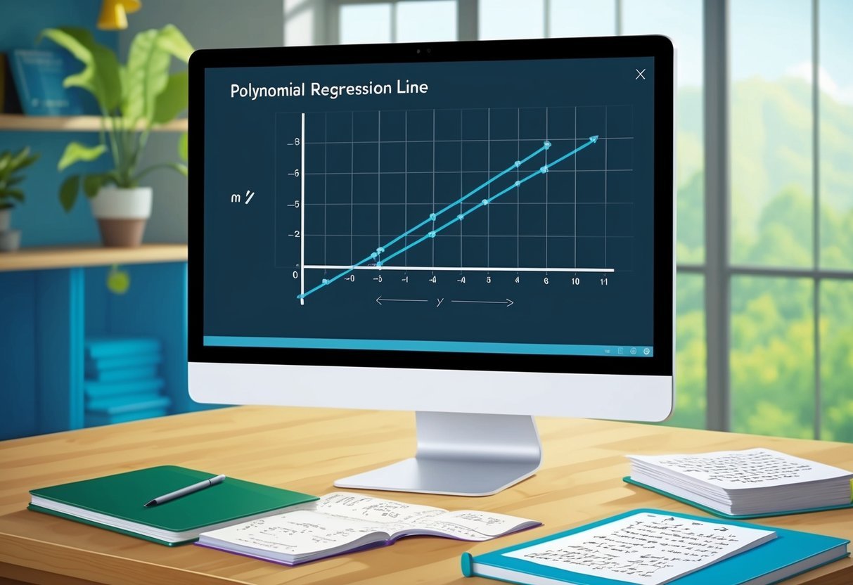
Plotting Polynomial Curves
One effective way to visualize a polynomial regression model is by plotting polynomial curves. Tools like Matplotlib can be used to create clear and informative plots.
When plotting, the x-axis represents the independent variable, while the y-axis shows the predicted values.
A curved line through the data points indicates the polynomial fit. Each polynomial feature, such as (x^2) or (x^3), adjusts the curvature, allowing complex relationships to be captured.
This visualization shows if the model aligns closely with the dataset, helping to identify overfitting or underfitting patterns.
Creating an interactive plot might involve scripts that let users toggle between different polynomial degrees. This helps in observing how changes in the polynomial degree impact the curve’s fit to the data.
A helpful practice is to overlay the original data points to provide context for how well the curve models the data.
Analyzing Residuals with Scatterplots
Residuals are differences between observed and predicted values. Scatterplots of residuals are a crucial tool for assessing model performance.
By plotting residuals on the y-axis and the independent variable on the x-axis, one can examine the spread and pattern of these residuals.
Scattered residuals without any distinct pattern suggest a good model fit. Patterns or structures in the residuals indicate issues, like missing polynomial features or outliers.
Matplotlib can be used to produce these plots, providing a straightforward way to check for bias or variances in the model.
Using a dataframe, analysts can compute residuals more efficiently, allowing for easy integration with visualization libraries. This makes it feasible to generate scatterplots quickly, facilitating a thorough examination of how well the regression curve fits the data across different segments.
Advanced Topics in Polynomial Regression
Polynomial regression can be a powerful tool to model complex relationships, but it also poses challenges. Understanding how to incorporate and navigate these complexities, along with utilizing cross-validation for better model performance, is essential for effective polynomial regression analysis.
Dealing with Complex Relationships
Polynomial regression helps model relationships that are not strictly linear. With polynomial terms, models can capture subtle curves in data.
One advantage is that it provides flexibility, allowing the inclusion of polynomial features like squares or cubes of predictor variables.
It’s important to balance model complexity. Adding too many polynomial terms increases the risk of overfitting, which means the model may perform well on training data but poorly on new data.
The degree of the polynomial should match the complexity of the relationship being modeled.
Introducing higher-degree polynomials can better capture patterns, but they also increase computational demands and instability. Practitioners must optimize the number of features used to ensure that the model remains efficient and predictive.
Incorporating Cross-Validation Methods
Cross-validation is crucial in polynomial regression to evaluate model performance and to prevent overfitting. It involves splitting the dataset into subsets, training the model on some parts called training sets, and testing it on others called validation sets.
One common method is k-fold cross-validation. It divides the data into k subsets and trains k times, each time using a different subset as the validation set and the remaining as training data.
This helps in ensuring that the model generalizes well to unseen data.
By using cross-validation, one can effectively determine how well a model’s predictions will perform in practice. It also aids in tuning the polynomial degree, as selecting the right degree impacts the model’s prediction quality. For more information on cross-validation techniques, see the University of Washington’s PDF lecture notes.
Comparative Analysis of Regression Models
Regression analysis involves comparing different models to find the best fit for a dataset. Key models in this field include linear regression and polynomial regression. These models vary in complexity and predictability, influencing their effectiveness in model evaluation.
Benchmarking Polynomial Against Linear Models
Linear models are simple and useful when the relationship between variables is straightforward. They predict an outcome by drawing a straight line through data points. However, in complex datasets, they might miss nuances.
Polynomial regression is more flexible, creating curved lines that better capture data patterns. This model fits non-linear trends, making it useful in waveform modeling.
Evaluating these models requires testing their predictions against real data and considering overfitting and underfitting risks.
A polynomial model, although more flexible, can overfit, capturing noise rather than true patterns. Meanwhile, linear models are often more robust with less risk of picking up on random noise.
Practical Applications of Polynomial Regression
Polynomial regression is widely used in data science for its ability to model non-linear relationships. Unlike linear regression, it can capture trends that bend and curve, making it suitable for complex data patterns.
A common application is in house price prediction. By considering variables like square footage, number of rooms, and location, polynomial regression can better fit the curved trend of prices over simple linear methods.
This approach avoids underestimating or overshooting price predictions, enhancing accuracy.
Another useful application is in the field of environmental science. Polynomial regression helps in modeling climate data and predicting temperature changes over time.
The non-linear relationship between temperature variables and environmental factors is effectively captured, leading to more reliable forecasts.
In engineering, it plays an important role in designing and analyzing systems, such as automotive performance. Factors like speed, load, and engine efficiency, which have non-linear interactions, benefit from this method to optimize performance metrics.
Marketing analytics also leverages polynomial regression to analyze market trends. Understanding consumer behavior involves recognizing the complex relationships between different marketing variables and sales outcomes.
This method helps in identifying patterns that impact decision-making processes.
Finally, biological sciences use polynomial regression to study growth patterns in organisms. By fitting the growth data with polynomial curves, researchers gain insights into developmental stages and other biological processes.
These examples showcase how polynomial regression is essential for capturing non-linear patterns across various fields.
More in-depth resources about techniques and applications can be found in articles discussing advanced polynomial regression techniques and machine learning methods.
Frequently Asked Questions
Polynomial regression is a powerful tool used to model complex relationships. Understanding real-world applications, the mathematical foundation, implementation steps, and evaluation methods can enhance its use.
What is an example of implementing polynomial regression in a real-world scenario?
Polynomial regression can model growth patterns in biology, such as predicting plant height based on time and environmental factors. By fitting a curve rather than a straight line, it can capture the nuances of natural growth processes.
How is the formula for polynomial regression derived and used?
The formula for polynomial regression is y = β0 + β1x + β2x² + … + βnxⁿ. This equation represents the dependent variable ( y ) as a polynomial function of the independent variable ( x ), where coefficients ( β ) are determined using statistical methods to best fit the data.
What are the steps to perform polynomial regression analysis in Python?
In Python, polynomial regression typically involves these steps: importing necessary libraries like NumPy and sklearn, preparing and normalizing the data, defining the polynomial features, fitting the model using linear regression, and evaluating the results. Using a library streamlines the process and ensures accurate calculations.
What are some disadvantages of using polynomial regression in predictive modeling?
A major drawback is that polynomial regression may lead to overfitting, especially with higher-degree polynomials in small datasets. It captures fluctuations that do not represent the underlying trend, resulting in a model that fails to generalize well to new data.
How do you evaluate the performance of a polynomial regression model?
Evaluating a polynomial regression model involves metrics such as R-squared, Mean Absolute Error (MAE), and Root Mean Square Error (RMSE). These metrics help determine the accuracy and reliability of the model in predicting outcomes based on test data.
What strategies can be employed to minimize overfitting in polynomial regression?
To minimize overfitting, one can use techniques like cross-validation, regularization (e.g., Ridge or Lasso), or opting for fewer polynomial terms.
Cross-validation splits the data to ensure the model performs well across unseen data, enhancing robustness.