
Fundamentals of Linear Regression
Linear regression is a basic yet powerful statistical method. It is used to model the relationship between two or more variables. This technique helps in predicting the output variable based on the input variables.
It’s a key concept in both statistics and machine learning.
Dependent Variable: This is what you aim to predict. Also known as the output variable, its value changes in response to changes in the independent variables.
Independent Variable: These are the input variables used to predict the dependent variable. Changes in these variables are assumed to influence the dependent variable.
In simple linear regression, there is one input and one output variable. The goal is to find the best-fitting line that represents the relationship between them. This line is often determined using the ordinary least squares method.
The formula for a simple linear regression model is:
[ Y = a + bX ]
- (Y) is the predicted output.
- (a) is the intercept.
- (b) is the slope of the line.
- (X) is the independent variable.
For multiple regression, more than one independent variable is used. This adds complexity but also improves prediction accuracy by considering multiple factors.
Understanding how variables are connected to each other is vital. With this knowledge, linear regression can be applied to diverse fields such as economics, finance, and social sciences. It helps to make data-driven decisions based on the observed relationships.
Understanding Simple Linear Regression
Simple linear regression is a method used to predict the relationship between two variables: one independent and one dependent. Key components like the regression line, slope, and intercept play a crucial role. It’s important to understand the assumptions such as linearity and normality that back this model.
Definition and Concepts
Simple linear regression models the relationship between two variables by fitting a straight line, known as the regression line, through data points. This line represents the best estimate of the dependent variable based on the independent variable.
Key components include the slope and the intercept. The slope indicates how much the dependent variable changes with a one-unit change in the independent variable. The intercept is the expected value of the dependent variable when the independent variable is zero.
In practice, simple linear regression helps in understanding how variables like income might impact another factor, such as spending habits. It provides a visual way to see correlation between the variables, showing whether changes in one variable are likely to affect the other.
Assumptions and Conditions
Simple linear regression relies on specific assumptions to be valid. One major assumption is linearity, which means the relationship between variables should be a straight line. The model also assumes homoscedasticity, meaning the variance of errors is consistent across all levels of the independent variable.
Another key assumption is normality of the residuals, where the differences between observed and predicted values should follow a normal distribution. These conditions help ensure the accuracy and reliability of predictions made by the regression model.
Understanding these assumptions is vital for interpreting results correctly. Violating these assumptions can lead to misleading conclusions, reducing the model’s effectiveness in predicting future outcomes.
The Mathematics Behind Regression
Understanding the mathematics of linear regression involves key concepts like the regression equation, calculating coefficients, and analyzing the mean and variance within the data. These elements work together to create a model that identifies relationships and patterns.
The Regression Equation
The regression equation is fundamental in predicting the relationship between variables. It is written as:
[ y = beta_0 + beta_1x + epsilon ]
Here, ( y ) is the dependent variable, ( x ) is the independent variable, ( beta_0 ) is the y-intercept, ( beta_1 ) is the slope, and ( epsilon ) is the error term. The slope indicates how much ( y ) changes for a one-unit change in ( x ). This equation helps to identify the best fit line that minimizes error, offering insights into the relationship between predictor and response variables.
Calculating Coefficients
Coefficients in the regression equation are calculated using methods like least squares. This technique minimizes the sum of the squared differences between observed and predicted values. The calculations involve solving:
[ beta_1 = frac{sum{(x_i – bar{x})(y_i – bar{y})}}{sum{(x_i – bar{x})^2}} ]
[ beta_0 = bar{y} – beta_1bar{x} ]
Where ( bar{x} ) and ( bar{y} ) are the means of the independent and dependent variables, respectively. Calculated coefficients provide direction and steepness of the line, which are essential for accurate machine learning algorithms.
Mean and Variance
Mean and variance are critical for evaluating the data’s distribution and spread. The mean describes the central tendency of the data, while variance measures its dispersion:
-
Mean: ( bar{x} = frac{sum{x}}{n} )
-
Variance: ( text{Var}(x) = frac{sum{(x_i – bar{x})^2}}{n} )
These metrics help in assessing the reliability and performance of the regression model. A large variance indicates more spread in the data, which might influence the line of best fit. Understanding these elements helps in creating more precise predictions.
Data Preparation for Regression Analysis
Preparing data for regression analysis involves crucial steps to ensure the accuracy and reliability of results. This process includes selecting an appropriate dataset and addressing any data quality issues that might impact the analysis.
Selecting a Dataset
Choosing the right dataset is essential for simple linear regression. The dataset should include a continuous dependent variable and an independent variable. Ideally, the data should be split into training and test datasets. This split enables a model to be trained on one portion and tested on another to evaluate performance.
A well-chosen dataset ensures the complexity of the model is appropriate for the problem. Before selection, one should outline the specific research question or hypothesis. Understanding the nature of the data will help in selecting a dataset that fits the requirements of the analysis.
Handling Data Quality Issues
Addressing data quality issues is key to robust regression analysis. The first step involves checking for missing values. Missing data can skew results, so options include removing rows with missing values or using imputation methods to fill gaps.
Outliers are another concern. They can disproportionately affect the slope of the regression line, thus careful scrutiny for them is vital. Conducting a preliminary analysis, such as calculating the mean and standard deviation, helps identify outliers.
Proper handling of these issues ensures the training data and test dataset yield reliable outcomes.
Visualizing Data to Recognize Patterns
Understanding how data points interact can reveal insights about patterns and trends. Visualizing data, especially with scatter plots and regression lines, helps in identifying the potential relationships and discrepancies.
Scatter Plots and Linearity
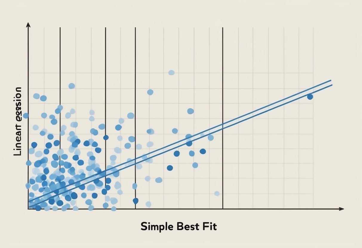
Scatter plots are a valuable tool for visualizing relationships between two variables. By plotting data points on a graph, one can easily see if there is a trend or pattern. Scatter plots are especially useful in identifying linearity, where points create a pattern that resembles a straight line.
To recognize this linearity, examining the distribution and spread of data points is important. If the points cluster tightly around a line, a linear relationship is likely present. This visual representation helps in assessing whether applying a simple linear regression model would be appropriate.
Best Fit Line and Residual Analysis
The line of best fit, or regression line, is drawn through data points to represent the relationship between variables. It minimizes the distance between itself and all points, indicating the trend. This line makes predictions more accurate and is central to understanding data patterns.
Residuals, the difference between observed values and predicted values by the line, help evaluate the line’s accuracy. Analyzing residuals through graphs shows if the model fits well or if there are patterns indicating issues. Lesser residuals typically suggest a better model fit, enhancing understanding of the model’s effectiveness.
Executing a Simple Linear Regression in Python
Simple linear regression helps find the relationship between two variables. By using Python, this method becomes efficient and easy to apply, especially with libraries that simplify the process. Below are ways to execute this algorithm using Python, including a demonstration.
Using Libraries and Frameworks
Python offers several libraries to implement simple linear regression efficiently. The most common library for this task is scikit-learn, which provides tools for building and training machine learning algorithms. Other libraries like NumPy and Pandas are crucial for data manipulation and preparation.
NumPy helps with numerical calculations, while Pandas handles data structures, making it easier to manage the training dataset.
To start, install the necessary libraries by running:
pip install numpy pandas scikit-learn
Matplotlib is useful for visualizing the results, helping to understand the linear relationship between variables. This library allows you to plot the regression line and identify how well it fits your data.
Code Example for Implementation
To execute a simple linear regression model in Python, first import the necessary packages:
import numpy as np
import pandas as pd
from sklearn.linear_model import LinearRegression
import matplotlib.pyplot as plt
Load your dataset, ensuring it is clean and ready for analysis. The training dataset should include the dependent and independent variables needed for the regression.
Create a LinearRegression object and fit it to your data, specifying the variables. This models the linear relationship:
model = LinearRegression()
model.fit(X_train, y_train)
Once the model is trained, make predictions:
predictions = model.predict(X_test)
Finally, use Matplotlib to visualize the results:
plt.scatter(X_test, y_test, color='blue')
plt.plot(X_test, predictions, color='red')
plt.show()
This example demonstrates how to implement the regression model, analyze results, and draw the regression line using Python and its libraries.
Simple Linear Regression in R
Simple linear regression is a statistical method used to model the relationship between two variables. It captures how a single dependent variable (response) changes as the independent variable (predictor) changes.
In R, this process is straightforward and can be done using the lm() function.
To perform simple linear regression in R, data should be prepared first. This includes ensuring the data meets key assumptions like linearity, independence, and homoscedasticity.
Visual tools like scatterplots can help check these assumptions.
The lm() function is used to create the regression model. The basic syntax is lm(y ~ x, data=mydata), where y is the dependent variable, x is the independent variable, and mydata is the dataset.
This function returns an object that contains the estimated coefficients, residuals, and other diagnostic information.
# Example in R
model <- lm(y ~ x, data=mydata)
summary(model)
The summary() function can be used to review the regression model. This includes the coefficients, R-squared value, and p-values, which help determine the strength and significance of the relationship.
Interpreting the output involves looking at the coefficients: the intercept (b0) and the slope (b1). The intercept indicates the expected value of y when x is zero, while the slope shows how much y changes for each unit increase in x.
Additional diagnostic plots and statistics can be evaluated using functions like plot() on the model object. These help check the fit and identify possible outliers or anomalies in the data. Such tools are crucial for refining and validating the model in real-world applications.
Algorithm Understanding for Optimization

Understanding key concepts like gradient descent, learning rate, and bias is crucial for optimizing linear regression algorithms. The following subtopics explain these concepts and how they impact optimization.
Exploring Gradient Descent
Gradient descent is an iterative optimization algorithm used to minimize a function by adjusting parameters. It calculates the gradient of the cost function, guiding the adjustments needed to find the optimal solution.
By moving in the direction of the steepest descent, the algorithm seeks to locate the function’s minimum. This process involves updating the coefficients of the model iteratively, reducing the difference between predicted and actual values.
For linear regression, this technique helps improve model accuracy by fine-tuning the line to best fit the data points.
Tuning the Learning Rate
The learning rate is a hyperparameter that determines the size of each step taken during gradient descent. A well-chosen learning rate enables efficient convergence to the minimum cost.
If the rate is too high, the algorithm might overshoot the minimum, leading to divergence.
Conversely, a learning rate that’s too low can result in a slow convergence process, requiring many iterations to reach an optimal solution.
Adjusting the learning rate is a sensitive task, as finding a balance helps achieve faster and more reliable optimization during model training.
Bias and Variance Trade-off
The bias and variance trade-off is a critical aspect of model building. Bias refers to errors introduced by simplifying the algorithm, which might cause underfitting when the model is too basic. In contrast, variance reflects the model’s sensitivity to small fluctuations in the training data, leading to overfitting.
Striking a balance between bias and variance ensures the model generalizes well to new data. Too much bias can result in poor predictions, while high variance can make a model overly complex, failing on unseen data.
Understanding and adjusting these factors can significantly improve the efficiency of the optimization process.
Evaluating Regression Model Performance
Model evaluation in regression focuses on analyzing residuals and various error metrics to assess how well the model predicts unseen data. This involves understanding both the leftover errors from predictions and metrics that quantify prediction quality.
Residual Analysis
Residual analysis is crucial for diagnosing a regression model’s performance. Residuals are the differences between observed and predicted values. Examining these helps identify patterns that the model might be missing.
Ideally, residuals should be randomly scattered around zero, indicating a good fit.
Plotting residuals can reveal non-linearity or heteroscedasticity. A histogram of residuals shows if errors are normally distributed. If residuals display a pattern, like funneling or a curve, it may suggest model improvements are needed, such as adding interaction terms or transforming variables to achieve linearity.
Error Metrics and Their Interpretations
Error metrics provide quantitative measures for evaluating a regression model.
Mean Squared Error (MSE) calculates the average of squared errors, emphasizing larger errors more than smaller ones.
Calculating the square root of MSE gives the Root Mean Squared Error (RMSE), which is easier to interpret because it’s in the same units as the response variable.
Standard Error quantifies the accuracy of predictions by measuring the average distance that the observed values fall from the regression line.
Lower values of RMSE and standard error indicate better predictive performance. These metrics help understand the model’s predictive power and guide model refinement to minimize errors.
Prediction and Forecasting with Regression
Prediction in linear regression involves using a model to estimate unknown values from known data. Simple linear regression uses a straight line to predict the dependent variable based on the independent variable. This approach is central to many fields, helping researchers and professionals make forecasts and informed decisions based on historical trends.
For many applications, forecasting can take different forms. For example, predicting future sales in a business relies on analyzing past sales data. Meanwhile, weather forecasting might predict temperature and rainfall based on various meteorological variables.
In finance, regression is often used to predict stock prices. Analysts create models based on past stock performance and external economic factors to make these predictions. This practice helps investors make strategic choices based on expected future returns.
Key components for accurate predictions include:
- Model Accuracy: Ensuring the model fits historical data well.
- Data Quality: Using reliable and relevant data.
- Variable Selection: Choosing the right independent variables.
Simple linear regression can extend to multiple linear regression, which uses more than one predictor. This provides a more detailed analysis and can improve prediction accuracy by considering multiple factors.
Making predictions in regression is about understanding relationships between variables and using that insight creatively to anticipate future outcomes. By combining statistical models with domain knowledge, this process helps in planning and decision-making across various industries.
Statistical Methods in Regression
Statistical methods play a critical role in regression analysis, helping to determine relationships and influences between variables. They include techniques such as hypothesis testing, which assesses the significance of regression results, and understanding correlation, which distinguishes between relationships.
Hypothesis Testing in Regression
Hypothesis testing is a statistical method used to verify if the relationship observed in regression analysis is statistically significant. It involves formulating a null hypothesis, which states there is no relationship between the independent and dependent variables, and an alternative hypothesis, suggesting a relationship exists.
In the context of simple linear regression, the t-test is often used to evaluate the significance of the regression coefficient. This test determines whether changes in the independent variable actively impact the dependent variable. A p-value is calculated to decide if the results can reject the null hypothesis with confidence.
Importantly, a low p-value (typically < 0.05) indicates strong evidence against the null hypothesis, suggesting the relationship is significant.
Another element in regression analysis is the y-intercept, which is tested to determine if the regression line passes through the origin or not, affecting the interpretation of data science results.
Understanding Correlation and Causation
Correlation and causation often confuse learners in regression analysis. Correlation measures how variables move together, meaning if one changes, the other tends to change too. The regression coefficient indicates the strength and direction of this correlation.
Yet, correlation does not imply causation. Just because two variables are correlated does not mean one causes the other to change. For instance, ice cream sales might correlate with temperature increases, but buying ice cream doesn’t increase temperatures.
Understanding this distinction is crucial in data science, where drawing incorrect conclusions about causation based on correlation can lead to misleading interpretations. Statistical methods help clarify these complex relationships, ensuring more accurate insights are gleaned from the data collected.
Advanced Topics in Linear Regression
When exploring advanced topics in linear regression, one key concept is multiple linear regression. This method extends simple linear regression by using two or more independent variables to predict a dependent variable. It helps in modeling more complex relationships in data sets, allowing a more comprehensive analysis.
Centering and scaling variables are crucial strategies in multiple linear regression. This involves adjusting predictor variables to have a mean of zero, which can improve the stability of the model, especially when interacting terms are present.
Interaction terms are used when the effect of one independent variable depends on the level of another variable. By including these terms, models can capture more complex relationships, reflecting real-world interactions between factors.
Another advanced aspect is polynomial regression. This is useful when the relationship between the variables is non-linear. By adding polynomial terms to the model, it can better fit non-linear data patterns.
Regularization techniques, such as Lasso and Ridge regression, help address issues of overfitting, particularly in models with many predictors. They work by adding penalties to the model, reducing the magnitude of coefficients, and improving the model’s predictive performance.
Handling multicollinearity is also significant in advanced linear regression. When independent variables are highly correlated, it can make estimates unreliable. Techniques like Variance Inflation Factor (VIF) can be used to detect and address these issues.
Model diagnostics are essential for ensuring the adequacy of a linear regression model. Techniques such as residual plots and goodness-of-fit measures help assess how well the model performs and identify potential areas of improvement.
Frequently Asked Questions

Simple Linear Regression is a fundamental statistical tool used to understand and predict relationships between two variables. It involves concepts like slope and intercept, making it valuable in research and practical applications.
What are the basic concepts and assumptions of Simple Linear Regression?
Simple Linear Regression involves modeling the relationship between an independent variable and a dependent variable. Key assumptions include a linear relationship, homoscedasticity, normal distribution of errors, and independence of observations.
How do you interpret the slope and intercept in a Simple Linear Regression model?
The slope indicates the change in the dependent variable for each unit change in the independent variable. The intercept represents the expected value of the dependent variable when the independent variable is zero.
What are the steps involved in performing a Simple Linear Regression analysis?
To perform Simple Linear Regression, start by plotting the data to check linearity, then estimate the coefficients using methods like ordinary least squares. Next, evaluate the model’s fit and validate assumptions through diagnostic checks.
How can Simple Linear Regression be applied in real-world research?
This model is widely used in fields such as finance and economics. It helps analyze the impact of variables like income or price on outcomes like sales or satisfaction, providing valuable insights for decision-making.
What are the common issues one can encounter with Simple Linear Regression, and how can they be addressed?
Common issues include non-linearity, heteroscedasticity, and autocorrelation. These can be addressed using transformations, weighted least squares, or adding relevant variables to the model.
How does Simple Linear Regression differ from multiple linear regression?
Simple Linear Regression uses one independent variable, while multiple linear regression involves two or more independent variables.
This allows for modeling more complex relationships, taking into account multiple factors affecting the dependent variable.