Understanding Linear Regression
Linear regression is a statistical method that helps explore the relationship between a dependent variable and one or more independent variables.
It serves an important role in many fields, including machine learning, where it is used to make predictions.
Fundamentals of Regression
At its core, linear regression assesses how a dependent variable changes with the alteration of independent variables. The main goal is to fit the best possible straight line through the data points to predict values accurately.
This line is called the regression line, represented by the equation (y = mx + b), where (y) is the dependent variable, (m) is the slope, (x) represents the independent variable, and (b) is the intercept.
The slope indicates the change in the dependent variable for a one-unit change in the independent variable. The intercept shows the expected value of the dependent variable when all independent variables are zero. Understanding this relationship helps in predicting and analyzing data trends effectively.
Linear Regression in Machine Learning
Linear regression is a fundamental algorithm in machine learning used for predicting continuous outcomes.
It involves training the model on a dataset to learn the patterns and applying those patterns to predict future outcomes.
Features, or independent variables, play a crucial role as they determine the model’s accuracy in predictions.
In machine learning, linear regression assists in tasks such as feature selection, emphasizing the importance of correctly identifying which features have a significant impact on the dependent variable.
It also requires checking the fit of the model through metrics like R-squared, which indicates how well the independent variables explain the variability of the dependent variable.
Preparing Data for Modeling
Effective data preparation is crucial for building accurate linear regression models. Key steps include data preprocessing to ensure data quality, handling categorical variables to convert them into numerical formats, and managing multicollinearity to prevent biased predictions.
Importance of Data Preprocessing
Before building a model, it’s important to preprocess the data to enhance its quality and usability. Techniques like filling missing values and detecting outliers are vital.
Pandas and NumPy are popular libraries for handling datasets. Preprocessing ensures that the independent variables are ready for analysis, reducing potential errors.
Feature scaling is another critical step, helping models perform better by putting all input features on a similar scale. Preprocessing lays a solid foundation for further analysis.
Handling Categorical Variables
Categorical variables represent data with labels rather than numbers. To use them in models, they must be transformed into numerical values. Techniques like one-hot encoding or label encoding can convert these variables effectively.
For instance, if using Python, the pandas library is essential for implementing these conversions. Understanding the dataset’s characteristics and using suitable encoding techniques ensures that the model can interpret and learn from these variables accurately.
Dealing with Multicollinearity
Multicollinearity occurs when independent variables in a dataset are too highly correlated, which can distort model predictions.
Checking the correlation between variables is essential. A high correlation coefficient may signal multicollinearity issues.
Techniques to address it include removing one of the correlated variables or using ridge regression, which adds a penalty to the coefficients.
It’s crucial to recognize and mitigate these issues to maintain the model’s reliability and interpretability.
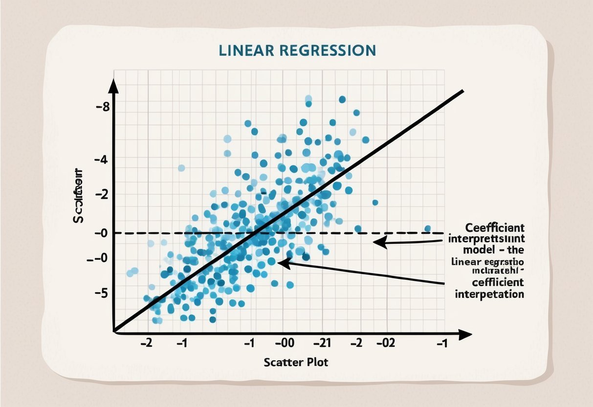
Interpreting Regression Coefficients
Interpreting regression coefficients involves understanding their meaning in relation to variables’ effects and statistical significance. Analyzing p-values determines if coefficients significantly influence a dependent variable, while reviewing regression tables provides quantitative insights into relationships between variables.
Coefficient Significance and P-Values
Coefficients measure the impact of each predictor variable on the response variable in a regression model. A positive coefficient indicates a direct relationship, meaning the dependent variable increases when the independent variable increases. A negative coefficient suggests an inverse relationship, where the dependent variable decreases as the independent variable increases.
P-values are critical for assessing the statistical significance of coefficients. They help determine whether a coefficient is statistically meaningful in the context of the model.
Generally, a p-value less than 0.05 indicates that the coefficient is significant, suggesting a true relationship between the predictor and response variable. It’s crucial to consider both the coefficient’s value and its p-value to draw accurate conclusions.
Reading a Regression Table
A regression table presents coefficients, standard errors, and p-values for each predictor variable, offering a concise summary of the model’s findings.
Each coefficient represents the expected change in the response variable for a one-unit change in the predictor, assuming all other variables remain constant.
Reading the regression table involves evaluating the size and sign of each coefficient to understand its effect direction and magnitude. Standard errors provide insight into the variability of coefficients, indicating the precision of the estimates.
By examining p-values alongside coefficients, one can identify which predictors significantly affect the response variable, guiding data-driven decisions in various fields like economics, psychology, and engineering.
Deploying Linear Regression Models
Deploying linear regression models involves transitioning from development to production, a critical step for practical application. This process includes carefully considering deployment challenges and ensuring a smooth transition. It is essential for scaling and integrating predictive capabilities into real-world environments.
From Development to Production
The journey from development to production in deploying linear regression models involves several important steps.
Initially, practitioners build and train models using Python libraries like scikit-learn. Python’s versatility makes it a popular choice for handling both the predictor variables and the response variable.
Once the model shows satisfactory results during testing, it needs to be deployed.
Deployment can involve frameworks like Flask, which allow models to become accessible through web applications. For example, linear models can be exposed as an API that applications can access. Containers play a vital role here. Tools like Docker allow these models to run in isolated environments, ensuring consistent performance across different systems.
Challenges in Model Deployment
Deploying machine learning models, particularly linear regression, comes with a number of challenges.
One major issue is ensuring that the model performs consistently in different environments. Discrepancies between the development and production settings can lead to unexpected results.
Additionally, scaling the model to handle numerous requests efficiently is vital.
Integrating these models smoothly into existing systems requires well-structured code and robust testing. This helps ensure the system’s reliability and response speed.
Monitoring the model’s predictions for accuracy in real-time is also crucial, as this allows for adjustments and retraining when necessary to maintain performance.
Deploying a linear regression model is not just about making it accessible, but also about maintaining its effectiveness over time.
Evaluating Model Performance
Evaluating the performance of a regression model involves checking residuals and assumptions, as well as assessing variance and model fit. This ensures that predictions are accurate and statistically significant. Understanding these concepts is crucial in regression analysis.
Residuals and Assumptions
Residuals are the differences between actual and predicted values. Analyzing them helps to check if the model assumptions hold.
In linear regression, these assumptions include linearity, homoscedasticity, independence, and normality.
A residual plot, where residuals are plotted against predicted values, aids in detecting patterns. If residuals are randomly scattered, it indicates a good fit. Non-random patterns may suggest errors in the model, such as omitted variables.
Violations of assumptions can impact the reliability of the model. For instance, non-linearity can lead to biased predictions. Correcting these issues involves transforming data or applying different modeling techniques.
Variance and Model Fit
Variance measures how much predicted outcomes vary. It is vital to evaluate the trade-off between bias and variance to ensure the model generalizes well.
A high variance might indicate overfitting, where the model captures noise instead of the true relationship.
Regression analysis often uses metrics like R-squared to determine model fit. R-squared indicates the proportion of variance explained by the model. Higher values suggest better fit, but very high values might hint at overfitting.
Reviewing variance also includes considering statistical significance. It helps confirm that the relationships the model captures are not due to random chance, enhancing confidence in the predictions.
Visualizing Linear Relationships
Visualizing linear relationships is essential in data science to understand the correlation between variables. This involves using visualization tools like Matplotlib and Seaborn to plot regression lines and observe relationships in the data.
Utilizing Matplotlib and Seaborn
Matplotlib and Seaborn are powerful libraries in Python for creating visualizations.
Matplotlib offers a variety of plots and is known for its flexibility and precision. Seaborn, built on top of Matplotlib, provides a high-level interface for drawing attractive and informative statistical graphics. These tools help in displaying linear relationships clearly.
Researchers and analysts often use these libraries to create scatter plots, which can show data points and provide an initial look at correlation between variables. Using Seaborn’s enhanced color palettes and themes adds an aesthetic layer to these visualizations, making patterns more noticeable.
Here is a simple code snippet for a scatter plot with a regression line using Seaborn:
import matplotlib.pyplot as plt
import seaborn as sns

# Example data
x = [1, 2, 3, 4, 5]
y = [2, 4, 5, 4, 5]

sns.set(style="whitegrid")
sns.regplot(x=x, y=y)
plt.xlabel("Independent Variable")
plt.ylabel("Dependent Variable")
plt.title("Scatter plot with Regression Line")
plt.show()
With these tools, users can effectively communicate linear relationships in their data.
Plotting the Regression Line
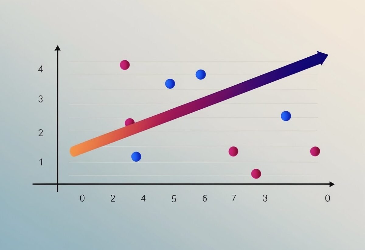
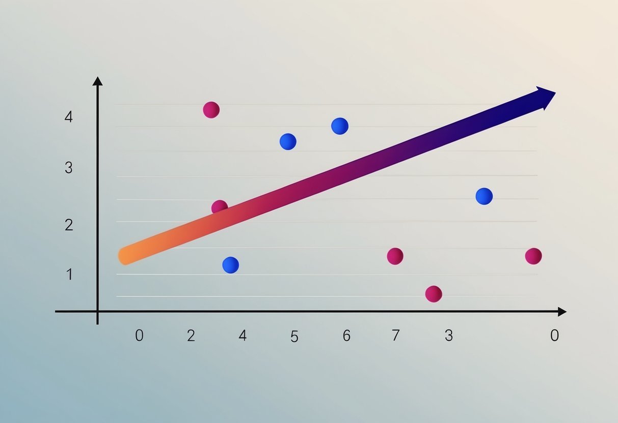
Plotting a regression line involves drawing a straight line that best fits the data points on a graph. This line represents the predicted relationship between the independent and dependent variables.
The goal is to minimize the distance between the data points and the line to reflect the strongest possible linear correlation.
When utilizing libraries like Matplotlib and Seaborn, it’s crucial to understand the plot parameters. Adjusting the axis, labels, and titles enhances the clarity of the visual output.
In Seaborn, the function regplot() automatically plots both the scatter plot of the data points and the regression line, which simplifies the creation of visual analysis.
To achieve precise and clear regression plots, data scientists often carefully choose the scale and labeling to ensure the regression line’s slope and intercept are visually meaningful. Accurate visualization aids in interpreting the model and communicating insights to stakeholders clearly and effectively.
Advanced Linear Regression Techniques
Advanced techniques in linear regression help improve model accuracy and interpretability. Regularization methods tackle overfitting, while polynomial and interaction features enhance model complexity.
Regularization Methods
Regularization is essential in preventing overfitting in linear regression models. By adding a penalty term to the cost function, these methods shrink the coefficients, aiding in more reliable models.
Two common techniques are Lasso and Ridge regression. Lasso regression uses L1 regularization, which encourages sparsity by reducing some coefficients to zero. This can be particularly useful for feature selection.
Ridge regression employs L2 regularization, penalizing large coefficients by adding the squared magnitudes of coefficients to the loss function. This helps in dealing with multicollinearity where independent variables are highly correlated. Advanced Regression Models also address these issues with code examples and templates.
Polynomial and Interaction Features
Enhancing linear regression models with polynomial and interaction features increases their ability to capture complex relationships.
Polynomial features can be created by raising independent variables to higher powers. This technique transforms linear models into nonlinear, allowing them to fit more complex patterns.
Interaction features multiply two or more variables together, capturing interactions between them. This is important when relationships between variables affect outcomes in a way that individual variables alone cannot capture.
By incorporating these features, regression models gain granularity, improving predictions and understanding of underlying data relationships. Incorporating such techniques in regression helps leverage the full potential of machine learning algorithms.
Using SHAP for Interpretation
SHAP offers a powerful tool for understanding how individual features contribute to model predictions.
By examining SHAP values, one gains insights into the significance and impact of different inputs.
Exploring Feature Contributions
SHAP focuses on evaluating feature contributions by assigning each feature a SHAP value. These values illustrate the strength and direction of a feature’s influence on predictions.
When a feature has a positive SHAP value, it boosts the prediction, while a negative value reduces it.
This interpretation helps uncover how features interact with each other and contributes to the final decision-making process.
For instance, in a machine learning model predicting house prices, the number of bedrooms might have a positive SHAP value, indicating it has a favorable impact on increasing the predicted price.
Conversely, age of the house might have a negative SHAP value, suggesting it lowers the price prediction.
Such explicit readings allow users to interpret coefficients meaningfully, spotting influential features with ease.
SHAP Values and Model Explanation
Visualizing SHAP values can enhance comprehension of predictive models.
Tools such as SHAP summary plots depict feature impacts dispersed across observations, making it easy to identify dominant features and their typical influences.
It’s important to note that SHAP is model-agnostic, which means it can be applied to interpret various machine learning models, from simple linear regression to complex techniques like gradient boosting and neural networks.
This versatility allows it to handle diverse data formats.
The calculated SHAP values offer a straightforward analysis of how each feature contributes to predictions, helping users and stakeholders grasp complex models.
Charts, such as the beeswarm plot, facilitate the visualization process by showing how feature effects aggregate across a dataset.
Using SHAP in this manner makes understanding intricate models accessible to a wider audience.
Modeling Considerations for Different Domains
When employing linear regression, it is essential to tailor the model to fit the specific needs and characteristics of the data from different industries and fields.
Whether the focus is on predicting economic trends or understanding student performance, each domain has unique requirements that must be addressed.
Industry-specific Applications
In various industries, linear regression is used to predict market trends, sales figures, and operational efficiencies. Regression analysis enables businesses to make data-driven decisions by examining the relationship between dependent and independent variables.
A well-constructed model can help anticipate future behavior based on historical data.
Different datasets across industries present diverse challenges. For instance, in retail, large and varied datasets can lead to complex models that require robust validation techniques.
In healthcare, data privacy and sensitivity increase the need for secure data handling and careful feature selection to ensure patient confidentiality while maintaining model accuracy.
Adapting linear regression to these challenges involves selecting relevant features and preprocessing data carefully. Industry norms and regulations often guide these decisions, necessitating domain expertise to ensure compliance and model reliability.
Educational Data and Exam Scores
In the educational sector, linear regression can play a crucial role in analyzing student performance and predicting exam scores.
By using data on classroom attendance, assignment completion, and previous grades, educators can identify patterns that influence student outcomes.
A typical dataset in this context includes student demographics, study habits, and academic history.
Careful handling of this data is important to preserve privacy while optimizing prediction accuracy.
In addition to privacy concerns, the variability in educational environments means that models must be adaptable and sensitive to different teaching methods and curriculum changes.
Interpreting coefficients in this domain helps educators understand the most influential factors on student success. This insight can lead to targeted interventions and personalized learning experiences, ultimately supporting improved educational outcomes.
Best Practices in Regression Modeling
Effective regression modeling involves careful feature selection and engineering, as well as ensuring quality and robustness in the model. These practices lead to more accurate predictions and better generalizations in machine learning applications.
Feature Selection and Engineering
Choosing the right features is crucial for building a strong regression model.
Irrelevant or redundant features can introduce noise and reduce the model’s predictive power.
Techniques like Lasso regression and Principal Component Analysis (PCA) help in selecting significant features while eliminating unnecessary ones.
Normalization and scaling are essential in preparing data for modeling. They ensure that all features contribute equally to the distance calculations in algorithms.
This is especially important in linear regression where units can vary widely across features.
Feature engineering often includes transforming variables, managing outliers, and creating interaction terms to better capture relationships within data.
Assuring Quality and Robustness
Ensuring the quality of a regression model involves thorough validation.
Techniques such as cross-validation help assess how the model performs on unseen data to prevent overfitting.
A common practice is to split the data into training and test sets. This helps evaluate if the model can generalize well to new data.
Robust regression techniques can handle data that contains outliers or non-normal distributions.
Methods like Ridge regression add penalty terms that help in managing multicollinearity among features.
It’s important to use diagnostic tools, such as residual plots and variance inflation factor (VIF), to identify and address potential issues that could affect the reliability of the model.
Revisiting the Importance of Coefficients
Linear regression coefficients play a crucial role in interpreting how changes in predictor variables impact the response variable. Understanding the size of effects and the associated uncertainty provides deeper insights.
Effect Size and Practical Significance
The magnitude of regression coefficients indicates the effect size of predictor variables on the response variable. A larger coefficient implies a more substantial impact on the outcome. Conversely, smaller values suggest minor influences.
Standardizing coefficients can make them comparable across variables measured in different units by bringing them to a similar scale. This highlights which predictors are the most significant to the model.
Understanding practical significance is key. For instance, even if a coefficient is statistically significant, its practical worth depends on the context.
A slight change in a variable might result in a large cost or benefit in real-world scenarios, making it essential to balance statistical results with real-life implications.
Confidence Intervals and Uncertainty
Confidence intervals provide insight into the uncertainty surrounding a coefficient estimate. By offering a range of likely values, these intervals help assess the reliability of the effect size.
A narrow confidence interval suggests a precise estimate, while a wide interval indicates more variability in the data.
Including the standard error in the analysis helps to evaluate the variability of the estimate.
A small standard error relative to the coefficient value signifies a more accurate estimate, while a larger one may indicate greater uncertainty.
Confidence intervals and standard errors together form a comprehensive picture of the reliability and accuracy of coefficients in a linear regression model.
Case Studies in Regression
Linear regression has various applications in both machine learning and data science. These real-world cases reveal how the estimated regression equation helps understand the relationship between variables in diverse fields.
Examining Real-world Applications
In the field of healthcare, linear regression often predicts patient outcomes based on factors like age, severity, and other health metrics.
For instance, a study with data from 46 patients evaluated how satisfaction with care linked to variables like age and condition severity. This analysis used the estimated regression equation to model these relationships, showing clear insights into patient experiences.
In business, linear regression aids in predictive analytics. Retail companies use it to forecast sales by analyzing data like advertising spend, seasonality, and economic indicators.
This helps in inventory management and strategic decision-making, optimizing operations based on expected demand.
Lessons Learned from Practical Deployments
Deploying regression models in practical scenarios often highlights the importance of model fit assessment.
Ensuring the accuracy of predictions depends on understanding the data and refining the regression analysis.
Challenges like multicollinearity, where independent variables are highly correlated, can affect model reliability. Addressing this requires careful data preparation and sometimes using techniques like ridge regression.
Another lesson is the significance of the coefficient interpretation. The coefficients provide insights into how changes in independent variables impact the dependent variable.
This is crucial for making informed decisions, such as how increasing marketing budget might increase sales in a business scenario.
Through these deployments, it’s clear that linear regression is not just about creating models, but also about extracting actionable insights from them.
Frequently Asked Questions
This section addresses common inquiries about deploying and understanding linear regression models. It covers the deployment process, the role of coefficients, and the significance of key statistical terms.
How can you deploy a linear regression model in a production environment?
Deploying a linear regression model involves various steps, including data preparation and model training. The model is often deployed using platforms that support integration, such as cloud services, which enable users to input new data and receive predictions. Testing and monitoring are crucial to ensure its effectiveness and reliability.
Can you explain the role of coefficients in a linear regression model?
Coefficients in a linear regression represent the relationship between each independent variable and the dependent variable. They indicate how much the dependent variable changes when a specific independent variable is altered, keeping others constant. Positive coefficients show a direct relationship, while negative coefficients suggest an inverse relationship.
What are the typical steps involved in performing linear regression analysis?
The process begins with data collection and preparation, followed by exploratory data analysis to understand data patterns. Next, the linear regression model is formulated and fitted to the data. After training, the model’s accuracy is validated using testing data, and finally, insights are interpreted and reported.
How do you explain the coefficient of determination in the context of a linear regression?
The coefficient of determination, denoted as R², indicates how well the independent variables explain the variability of the dependent variable. An R² value closer to 1 suggests a good fit. It measures the proportion of variance in the dependent variable predicted by the model, reflecting the model’s explanatory power.
In what scenarios is multiple linear regression preferred over simple linear regression?
Multiple linear regression is preferred when there are multiple independent variables influencing the dependent variable and when capturing the effects of each is essential. This approach is ideal for complex data sets where considering just one independent variable would lead to oversimplification and missed relationships.
What is the process for interpreting the correlation coefficient in a linear regression study?
The correlation coefficient measures the strength and direction of the relationship between two variables.
In a linear regression context, it helps assess how changes in one variable might predict changes in another.
A value near 1 or -1 indicates a strong relationship, while a value around 0 suggests little to no linear correlation.