Author: JW

Foundations of Linear Algebra

Linear algebra is essential in data science. It provides tools to manage and analyze data effectively. The key concepts include matrices and vectors, which are used extensively in solving linear equations.

Understanding Matrices and Vectors

Matrices and vectors are fundamental in the field of linear algebra. A matrix is a rectangular array of numbers arranged in rows and columns. They are used to perform linear transformations and organize data.

Matrices can represent datasets, where each row is an observation and each column is a feature.

A vector is a one-dimensional array of numbers. Vectors can represent points in space, directions, or quantities with both magnitude and direction. They are crucial in operations like vector addition or scalar multiplication. These operations help in manipulating and analyzing data points, which are central to data science tasks such as machine learning and computer graphics.

Understanding these two elements enables one to perform more complex tasks like matrix multiplication. Matrix multiplication allows combining data transformations and is vital in applications such as neural networks.

Fundamentals of Linear Equations

Linear equations are expressions where each term is either a constant or the product of a constant and a single variable. In data science, systems of linear equations are used to model relationships among variables.

These equations can be written in matrix form, which simplifies their manipulation using computational tools. Matrix techniques, such as Gaussian elimination or the use of inverse matrices, are typically employed to find solutions to these systems.

Solving them is crucial for regression analysis, optimization problems, and various algorithms in data science.

Linear algebra provides methods to efficiently handle these equations, enabling data scientists to make accurate predictions and optimize models. This skill set is pivotal in creating machines that learn from data, making it a cornerstone of modern data science practices.

Matrix Arithmetic for Data Science

Matrix arithmetic plays a pivotal role in data science by helping to handle complex data structures and perform various calculations. Concepts like matrix multiplication and inverses are crucial for tasks such as solving systems of equations and enabling smooth operations in machine learning algorithms.

Matrix Multiplication Relevance

Matrix multiplication is a core operation in linear algebra, connecting different mathematical expressions efficiently. In data science, it allows practitioners to combine linear transformations, which are essential for building models and manipulating datasets.

Consider a scenario where two matrices, A and B, represent data inputs and transformation coefficients, respectively. Their product, AB, results in a transformation that applies to the data.

Matrix multiplication, hence, becomes vital in expressing complex transformations easily. It helps in various applications, such as optimizing linear regression algorithms.

In machine learning, for example, the weights of layers in neural networks are often represented as matrices. Efficient computation of matrix products speeds up model training and evaluation processes. Matrix multiplication isn’t just a mathematical necessity; it’s a practical tool enabling data scientists to process large datasets and apply sophisticated algorithms.

Inverse Matrices and Systems of Equations

The inverse of a matrix is another fundamental concept with significant benefits in data science. If matrix A has an inverse, denoted as A⁻¹, then multiplying these yields the identity matrix. This property is crucial for solving systems of equations.

For example, to solve Ax = b for x, where A is a matrix and b is a vector, the solution can be expressed as x = A⁻¹b, provided A is invertible.

This solution method is often used in linear regression models and other statistical analyses, supporting efficient computation without reiterating distinct algebraic steps.

In data science, using inverse matrices helps streamline the process of finding solutions to numerous linear equations simultaneously. It also supports other computations, like eliminating redundancies in datasets, making them more manageable for further analysis.

Algebraic Methods and Algorithms

Understanding algebraic methods and algorithms is crucial for solving systems of equations in linear algebra. These methods allow for efficient solutions, essential for data science applications.

The Elimination Method

The elimination method, often called Gaussian elimination, is a systematic way to solve systems of linear equations. It involves manipulating the equations to eliminate variables, ultimately finding the values of all unknowns.

This method is preferred because it can be used for systems with multiple variables and equations. The process starts by rearranging the equations and subtracting multiples to eliminate one variable at a time.

Practicing this technique helps in understanding how changes in one part of a system affect the entire solution. Its structure reduces errors and simplifies the solution process, providing clarity and consistency.

Row Echelon Form and Its Significance

Row echelon form (REF) is a key concept in solving linear equations using matrices. A matrix is in row echelon form when it has a staircase-like structure, where each leading entry (or pivot) is to the right of the one above it.

Achieving REF through row operations simplifies complex systems and makes it easier to interpret solutions quickly. This method highlights dependent and independent equations, assisting in identifying and resolving inconsistencies.

Learning REF is vital for students and professionals as it forms the basis of more advanced techniques like the reduced row echelon form, which further refines solutions in matrix problems. Understanding these concepts aids in developing a deep comprehension of algebraic problem-solving.

Solving Systems of Linear Equations

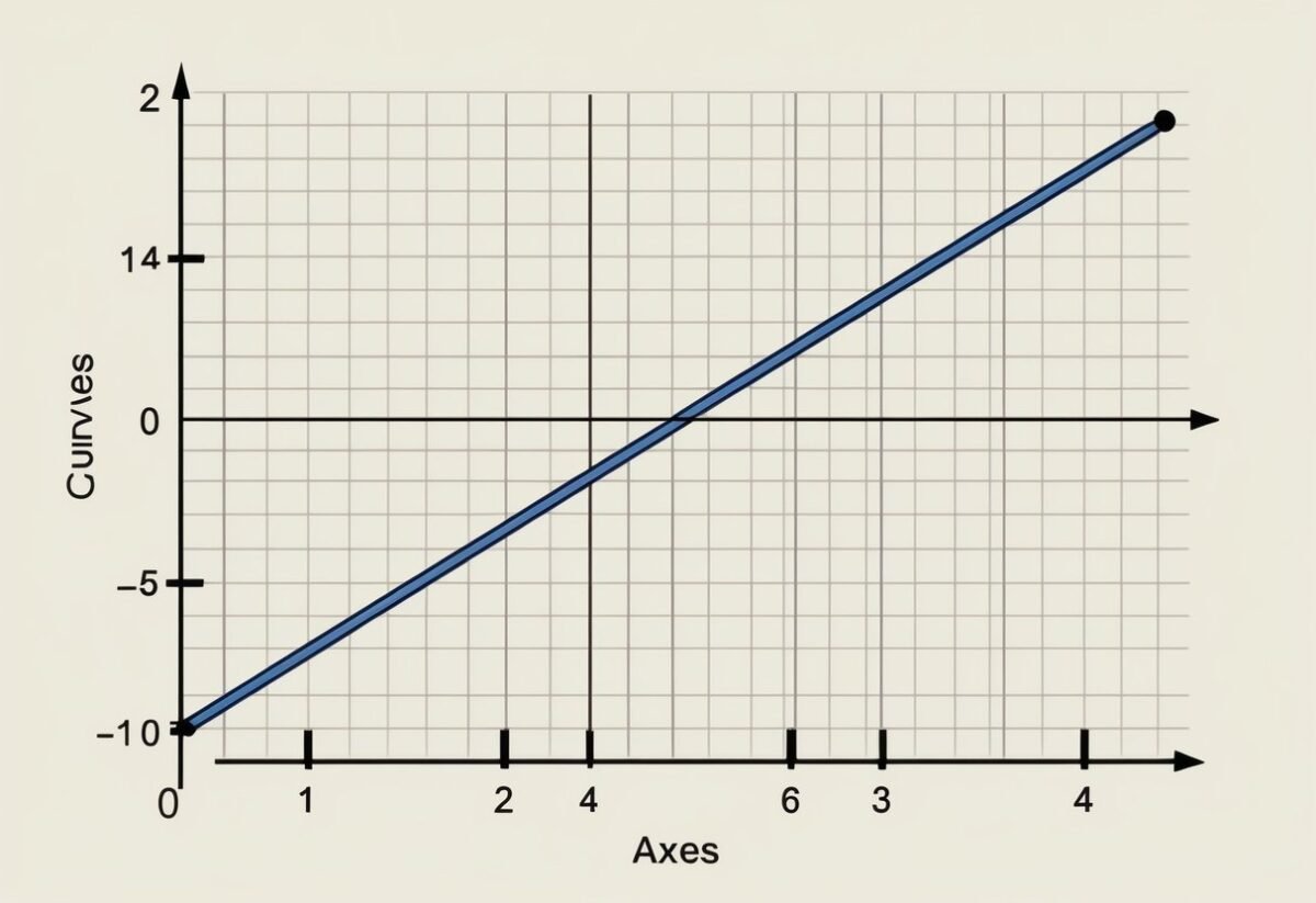
When solving systems of linear equations, it’s essential to understand the different outcomes. A system can have a unique solution, infinite solutions, or no solution at all. Each outcome depends on the equations’ alignment and structure. Using matrix form helps visualize and solve these systems efficiently.

Unique, Infinite, and No Solutions

Linear systems often result in different solution types. A unique solution exists when the equations intersect at a single point. This occurs when the matrix representing the system has full rank.

Infinite solutions arise if the equations are the same line or plane, meaning they overlap completely. In this case, the system’s rank is less than the number of variables, and all variables in the solution depend on a free variable.

When there is no solution, the equations represent parallel lines or planes that never intersect. In this situation, the system is inconsistent, often due to contradictory equations, resulting in an empty solution set.

Matrix Form Representation

Representing linear systems in matrix form simplifies the process of finding solutions. The system is expressed as a matrix equation, (AX = B), where (A) is the coefficients matrix, (X) is the variable vector, and (B) is the constants vector.

This form makes it easier to apply row operations to reach row echelon or reduced row echelon form. Solving for (X) requires methods like Gaussian elimination or matrix inversion, if applicable.

Efficient computation using matrices is vital in data science for solving systems that arise in tasks like linear regression and data transformation.

Understanding Vector Spaces

Vector spaces are essential in linear algebra and data science. They provide a way to structure data using vectors and transformations. Understanding how these spaces work helps in solving complex problems and developing efficient algorithms.

Span, Basis, and Dimension

In vector spaces, the span refers to all possible combinations of a set of vectors. These vectors can create different points in the space, allowing representation of various data. If vectors are combined and can form any vector in the space, they are said to span that space.

The basis of a vector space is a set of vectors that are linearly independent and span the entire space. A basis includes the minimum number of vectors needed without redundancy. Identifying the basis is crucial because it simplifies the representation of vectors in that space.

The dimension of a vector space is determined by the number of vectors in the basis. This number indicates how many coordinates are needed to specify each vector in the space, which directly impacts operations such as data representation and transformations.

Linear Independence in Data Science

Linearly independent vectors do not overlap completely in their contributions. No vector in the set can be made using a combination of the others.

This property is crucial in data science for ensuring that the data representation is efficient and non-redundant.

In applications like machine learning, using linearly independent vectors avoids unnecessary complexity and redundancy. Algorithms function better with data framed in simplified, independent sets.

Data transformation techniques often rely on ensuring and maintaining linear independence. Understanding these concepts helps in building models and representations that are both robust and easy to work with.

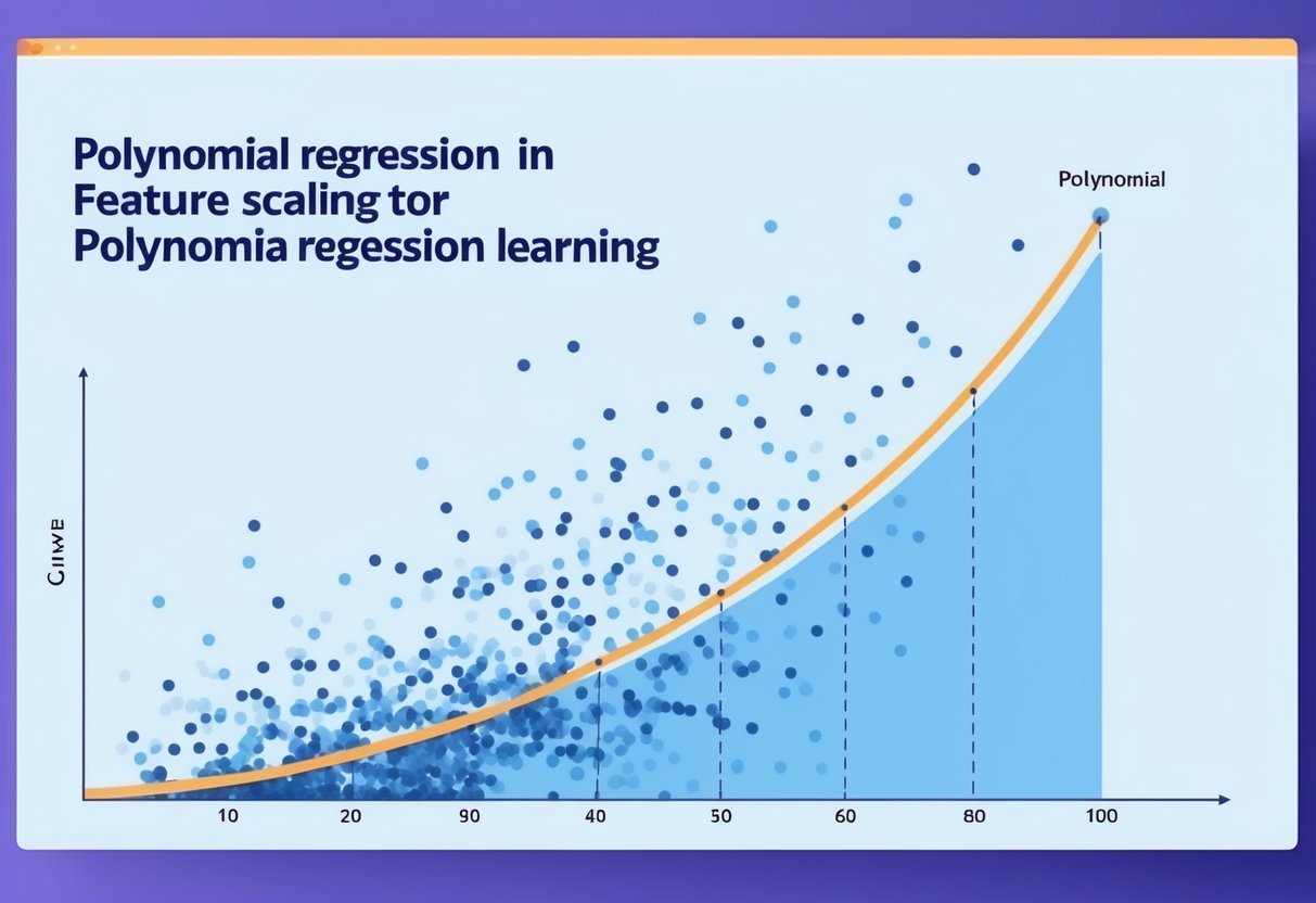
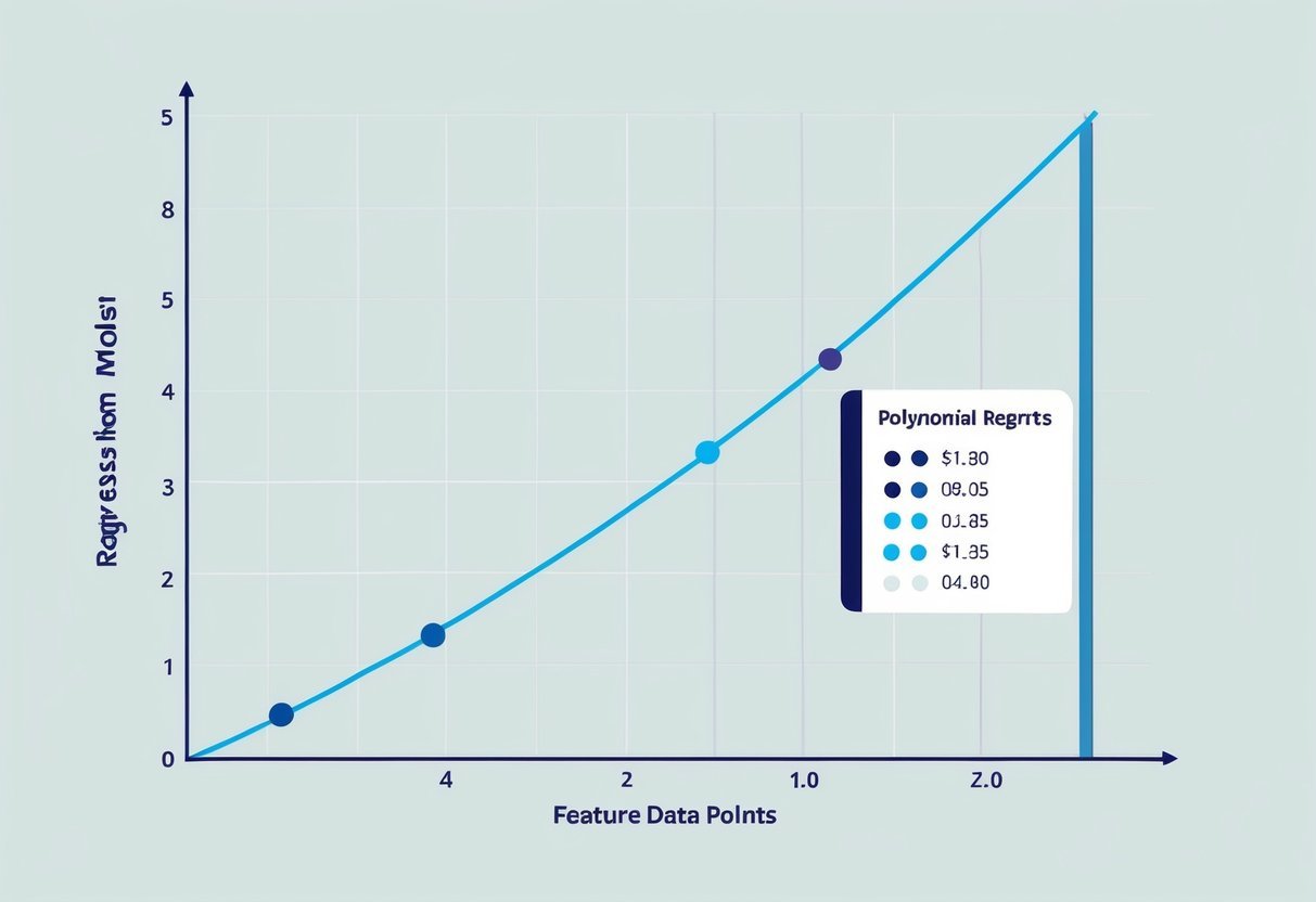
Dimensionality Reduction Techniques

Dimensionality reduction is a crucial part of data science. It helps to simplify datasets while retaining essential information. This section explores two major techniques: Principal Component Analysis (PCA) and Singular Value Decomposition (SVD).

Principal Component Analysis (PCA)

Principal Component Analysis is a technique used to reduce the number of variables in a dataset. It does this by identifying key components that capture the most variance from the data.

This method transforms the original variables into a set of new, uncorrelated variables known as principal components. PCA is useful for simplifying data, reducing noise, and visualizing complex datasets.

The first principal component accounts for the most variance, with each subsequent component explaining additional variance. PCA is widely used in image compression and noise reduction due to its ability to retain significant features from the data. To learn more, check out this article on dimensionality reduction techniques.

Singular Value Decomposition and Its Applications

Singular Value Decomposition (SVD) is another powerful method for dimensionality reduction. It factorizes a matrix into three simpler matrices to reveal underlying patterns in the data.

SVD is often used for data compression and noise reduction, similar to PCA. It can also assist in solving systems of equations and enhancing data representation.

SVD breaks down data into singular values and vectors, providing insight into the data’s structure. This makes it a valuable tool in fields like signal processing and collaborative filtering. For deeper insights on SVD’s applications, explore this guide.

Eigenvalues and Eigenvectors in Machine Learning

Eigenvalues and eigenvectors are essential tools in machine learning, offering insights into data through transformations. They help simplify complex datasets and uncover hidden structures, enabling better understanding and predictions.

Calculating Eigenvalues and Eigenvectors

Calculating eigenvalues and eigenvectors involves solving the characteristic equation of a square matrix. The equation is obtained by subtracting a scalar, often denoted as lambda (λ), multiplied by the identity matrix from the original matrix. The determinant of this expression then equals zero.

Solving this determinant provides the eigenvalues.

Once the eigenvalues are found, solving linear equations involving these values and the original matrix helps determine the corresponding eigenvectors.

Eigenvectors are non-zero vectors that remain in the same direction when linear transformations are applied. These vectors are crucial for machine learning as they form a basis to reshape data and identify patterns.

Significance of Eigenbases

Eigenbases refer to the set of eigenvectors that form a basis for a vector space. In machine learning, they are particularly significant when working with data transformations, like in Principal Component Analysis (PCA).

By converting the correlated variables of a dataset into a set of uncorrelated eigenvectors, or principal components, data can be reduced efficiently.

This transformation amplifies the most important features while suppressing noise, which leads to improved model performance. Eigenbases enhance the performance of algorithms by offering simplified representations that retain essential information, which is beneficial in processing large datasets and in artificial intelligence applications.

Understanding and using eigenbases in machine learning allows for the construction of models that are both efficient and insightful.

Eigenbases play a vital role in ensuring that models are built on robust mathematical foundations, contributing to the success and accuracy of machine learning applications.

Real-World Applications of Linear Algebra

Linear algebra plays a significant role in data science. It is vital in areas like optimizing algorithms in machine learning and enhancing computer vision through image processing and compression.

Optimization for Machine Learning

In machine learning, optimization is critical for improving model performance. Linear algebra helps in solving optimization problems efficiently.

It is used in algorithms like gradient descent, which minimizes error in predictive models by finding the optimal parameters.

Large datasets in machine learning are often represented as matrices or vectors. This allows for efficient computation of operations needed for training models.

Matrix factorization techniques, such as Singular Value Decomposition (SVD), are essential for tasks like recommender systems. These techniques decompose data matrices to reveal patterns and enhance prediction accuracy.

This approach improves processing speed and performance in real-world scenarios by managing large-scale data with precision.

Computer Vision and Image Compression

Linear algebra is fundamental in computer vision and image compression. In this area, transforming images into different formats involves operations on matrices.

Images are often stored as matrices of pixel values, and operations like edge detection rely on matrix operations to highlight features.

Compression algorithms like JPEG use linear algebra techniques to reduce file size without losing significant quality.

Discrete Cosine Transform (DCT), a key technique, converts image data into frequency components to compress it efficiently.

These practices enhance both storage efficiency and image processing speed, making them essential in real-world applications where large amounts of image data are involved. This results in faster transmission and reduced storage requirements, which are critical in fields like medical imaging and streaming services.

The Role of Linear Algebra in AI Models

Linear algebra is crucial in AI, especially in handling data arrays and computations. It forms the backbone of techniques used in neural networks and deep learning, enabling efficient processing and understanding of complex data.

Understanding Neural Networks

Neural networks are a central part of AI models. They use linear algebra to model relationships between inputs and outputs. Each connection in a neural network can be described using vectors and matrices.

Matrix operations help in the transformation and weighting of inputs, which are key in adjusting model parameters.

This adjustment process is essential for training models to accurately predict outcomes.

Neural networks perform calculations through layers, where each layer applies linear transformations to output data.

A good grasp of vectors and matrices helps in optimizing these networks. It not only aids in understanding the spread of data but also in how machine learning models make predictions.

Linear Algebra in Deep Learning

Deep learning builds on the concepts of neural networks by adding more layers and complexity. Each layer’s operations are defined by linear algebra concepts, which include matrix multiplication and vector addition.

These operations allow deep learning models to process high-dimensional data efficiently.

Using linear algebra, deeplearning.ai algorithms can handle diverse tasks, from image recognition to language processing.

Understanding matrix decomposition is key, as it simplifies complex data structures into manageable forms. This is essential in improving computation speed and accuracy.

Linear transformations and other techniques allow models to learn by adjusting weights and biases across layers, leading to more precise predictions.

Programming Linear Algebra Solutions

When working with linear algebra in data science, programming plays a crucial role. Using Python, data scientists can solve systems of equations more efficiently through libraries and carefully implemented algorithms. Understanding which tools and methods to apply can significantly optimize workflows.

Linear Algebra Libraries in Python

Python offers several libraries tailored to linear algebra, making it a popular choice for data scientists. NumPy is fundamental, providing array operations and matrix math. It is often used for handling large datasets efficiently.

SciPy builds on NumPy, offering advanced linear algebra operations. Functions like scipy.linalg.solve() allow for direct solutions to linear equations.

For more specialized needs, SymPy handles symbolic mathematics, useful for deriving formulas or solving equations exactly.

These libraries help automate complex calculations, reducing error and saving time. Mastery of them equips data scientists with powerful tools for tackling challenging problems.

Implementing Algorithms for Efficiency

Efficient algorithms are key to solving linear systems quickly. The Gauss-Jordan elimination method is widely used for its ability to simplify matrices to row-echelon form, making solutions apparent.

In contrast, LU decomposition breaks a matrix into lower and upper triangular forms, helping to solve equations more systematically.

Python’s libraries implement these algorithms with functions like numpy.linalg.solve(). Using these allows data scientists to focus on analysis rather than computation.

Additionally, optimizing these algorithms involves considering computational complexity, which is crucial for processing large datasets efficiently and effectively.

Effective programming practices in Python ensure precise and fast solutions, integral to data science applications.

Statistic and Calculus Interplay with Linear Algebra

Statistics and calculus play crucial roles in understanding and optimizing linear algebra applications. They interact closely in areas like linear regression and optimization techniques, providing the tools needed for data science.

Linear Regression and Correlation

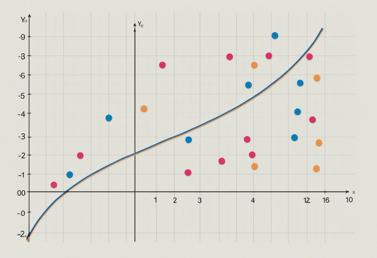
Linear regression uses calculus and linear algebra to find relationships between variables. It involves finding a line that best fits data points, using the least squares method to minimize error. Correlation measures the strength and direction of this relationship between two variables.

Linear algebra techniques help solve these regression equations through matrices. A key concept here is the matrix equation Y = Xβ + ε, where Y is the response vector, X is the design matrix, β is the coefficient vector, and ε is the error term.

By utilizing these equations, data scientists can predict trends and make informed decisions.

The Calculus Behind Optimization

Optimization in data science often relies on calculus concepts applied through linear algebra. Calculus, particularly derivatives, helps determine the minimum or maximum values of functions, essential for optimization.

In machine learning, gradient descent is a method used to find the minimum of a function by iteratively moving in the direction of the steepest descent as defined by calculus.

The calculations benefit significantly from linear algebra techniques, where large systems can be optimized efficiently. Understanding these interactions allows for better model performance and more precise predictions, improving how algorithms learn and adapt.

Advanced Matrix Concepts in Data Science

Matrices play a crucial role in data science, especially in solving complex problems like classification and noise reduction. Key concepts involve using matrix operations to transform and understand data more effectively.

Classification Through Matrices

In data science, classification tasks often use matrices to organize and process input data. Matrix operations, such as multiplication and addition, are used to transform data into formats suitable for algorithms.

By representing data as matrices, it becomes easier to implement classification algorithms like logistic regression, which rely on linear combinations of input features.

Matrices can simplify the computation involved in feature extraction. This process helps algorithms identify the most relevant aspects of the data, improving precision and efficiency.

Techniques such as Singular Value Decomposition (SVD) aid in reducing the dimensionality of data, allowing classifiers to focus on the most valuable features.

This mathematical approach ensures that classifiers are not overwhelmed by unnecessary information and can perform at their best.

Covariance Matrices and Noise Reduction

Covariance matrices are vital for understanding data variability and relationships between different data dimensions. They help in assessing how one feature varies in relation to others.

This understanding is crucial in data science for recognizing patterns and making predictions.

Noise reduction often involves manipulating covariance matrices to filter out irrelevant information. By focusing on the principal components identified in these matrices, data scientists can maintain the integrity of the dataset while reducing noise.

Techniques like Principal Component Analysis (PCA) rely on covariance matrices to transform data and enhance signal clarity. These methods are essential for maintaining the accuracy and reliability of models, especially when dealing with large datasets.

Accurate covariance analysis helps ensure that only meaningful variations are considered in data modeling.

Frequently Asked Questions

Understanding linear algebra is vital for data science, particularly in solving systems of equations. It facilitates model optimization and data manipulation using a wide range of mathematical techniques.

What are the most crucial linear algebra concepts to understand for data science?

Essential concepts include matrix multiplication, vector addition, and understanding eigenvalues and eigenvectors. These are foundational for algorithms like principal component analysis and support vector machines.

How does one apply linear algebra to solving real-world data science problems?

Linear algebra is used for data transformations and dimensionality reduction, which helps in efficiently handling large datasets. Techniques like gradient descent benefit from these mathematical principles.

Can you recommend any comprehensive textbooks on linear algebra geared towards data scientists?

A recommended textbook is “Linear Algebra and Its Applications” by Gilbert Strang. It offers practical insights with a focus on applications relevant to data science.

What online courses would you suggest for mastering linear algebra in the context of machine learning?

Courses like “Linear Algebra for Machine Learning and Data Science” on Coursera cover essential applications using tools like Python.

How important is proficiency in linear algebra for performing well in data science roles?

Proficiency in linear algebra is crucial. It enhances the ability to build, understand, and refine machine learning models, making it a valuable skill in data science roles.

What are some effective strategies for learning the algebraic method to solve systems of linear equations?

One effective strategy is to practice using software tools like MATLAB or Python. These tools provide hands-on experience in visualizing and solving equations. They also reinforce theoretical knowledge through application.

Understanding the Basics of Python Inheritance

Inheritance is a key feature of object-oriented programming in Python. It allows a subclass to inherit methods and properties from a base class or superclass. This promotes code reusability and a clear hierarchy in the code.

There are several types of inheritance in Python:

1. Single Inheritance: This is when a subclass inherits from one base class.

2. Multiple Inheritance: A subclass inherits from more than one base class. This allows for greater flexibility but can introduce complexity.

3. Multilevel Inheritance: A chain of inheritance where a class is derived from another derived class.

4. Hierarchical Inheritance: Multiple subclasses inherit from a single base class.

5. Hybrid Inheritance: Combines two or more types of inheritance. It’s a complex form and is commonly used in advanced scenarios.

A class can be created using simple syntax. Here is a basic example:

class Base:
    def greet(self):
        return "Hello from Base!"

class Sub(Base):
    pass

sub_instance = Sub()
print(sub_instance.greet())  # Output: Hello from Base!

In this example, Sub inherits from Base, demonstrating single inheritance. The Sub class can use the greet method from the Base class without redefining it.

For more information, you can delve into Python Inheritance Explained and read examples on Python Inheritance at W3Schools. These resources offer valuable insights into the various types of inheritance in Python.

Defining Classes and Subclasses in Inheritance

In Python, inheritance is a key feature that lets a class inherit properties and behavior from another class. This section explores how to create a parent class, derive subclasses, and understand different inheritance types using Python.

Creating a Base Class

A base class, also known as a parent class, is the starting point for inheritance. It defines methods and properties common to all derived classes. When you create a parent class, it establishes a blueprint. For example, a base class named Animal might have methods like eat() and sleep(). These methods will then be available in any subclass.

Using a base class helps in maintaining and updating code. If a method in the base class needs changes, the change automatically reflects in all subclasses. This makes the code more efficient and easier to read. A base class is typically defined like this:

class Animal:
    def eat(self):
        print("Eating")

Deriving Subclasses from a Base Class

Subclasses, or derived classes, extend the functionality of base classes. To create a subclass, it inherits all methods and properties from the parent class. In Python, a subclass is created using syntax like this:

class Dog(Animal):
    def bark(self):
        print("Barking")

Here, Dog is the child class of Animal. It inherits all behaviors of Animal and adds new methods like bark(). Subclasses can also override methods of the parent class to provide specific implementations. Such flexibility in programming allows for increased reuse and organized code.

Understanding Single and Multiple Inheritance

Single inheritance involves a child class inheriting from only one parent class. It’s the most straightforward form. For example, if Bird is a subclass of Animal, it follows single inheritance.

Multiple inheritance, on the other hand, allows a class to inherit from multiple parent classes. In Python, this is possible, though it can introduce complexity. Python handles method conflicts in multiple inheritance using Method Resolution Order (MRO). This controls the order in which methods are looked up.

For multiple inheritance:

class Bird(Animal, FlyingObject):
    pass

Here, Bird inherits from both Animal and FlyingObject, combining features from both.

Exploring Multilevel and Hierarchical Inheritance

Multilevel inheritance involves a class deriving from a child class, creating a chain. For instance, Sparrow might inherit from Bird, which in turn inherits from Animal. The hierarchy develops as:

• Animal (Base)
• Bird (Derived from Animal)
• Sparrow (Derived from Bird)

Hierarchical inheritance, however, involves multiple derived classes coming from a single base class. The code keeps the relationships clear and supports broad reuse of the base class’s methods.

Both types of inheritance enhance versatility by allowing shared properties across multiple classes, maintaining the ease of modification and expansion.

The Role of Constructors in Inheritance

Constructors play a crucial role in Python inheritance by initializing objects and setting up the initial state of an object. Inheritance allows classes to inherit properties from other classes, and constructors are key to ensuring that this process works smoothly and efficiently.

Using Constructors in Base Classes

In Python, a constructor is a special method called __init__, which is used to initialize objects. When a class inherits from another, the base class constructor can be invoked to ensure that the base class is properly initialized. This can be important for setting up attributes and behaviors that the child class will also use.

For instance, if a Student base class has an __init__ method to initialize names and IDs, a derived class like Marks might need these attributes to correctly store student data. Calling the constructor of the base class ensures that all necessary properties are set, facilitating the creation of an integrated object model. For more details, you can refer to constructor role in inheritance.

Constructor Overriding and Inheritance

In cases where the derived class requires a different approach to initialization, overriding the constructor can cater to those needs. By redefining the __init__ method, the derived class can initialize additional properties or modify how base properties are set.

However, it’s essential to call the constructor of the parent class using the super() function to maintain consistency and avoid duplicating code. This function provides a reference to the parent class, enabling the child class to build upon its existing constructors. Failing to call the base constructor might result in missed initialization processes, impacting the stability of the application. More information on this can be found in the Python Land Tutorial.

Method Overriding and Method Overloading

Method overriding and method overloading are two important concepts in Python related to object-oriented programming. They allow developers to write more flexible and maintainable code by customizing how objects behave.

Overriding Methods in Subclasses

Method overriding occurs when a subclass provides a new implementation for a method that is already defined in its superclass. This concept is crucial in object-oriented programming as it enables subclasses to offer specialized behaviors. When the method in the superclass is called, the version in the subclass takes precedence. This technique is often used to tailor methods to the specific needs of the subclass. For instance, if a superclass has a method for displaying data, a subclass might override it to present data in a different format. More information on method overriding can be found in a GeeksforGeeks article.

Difference Between Overriding and Overloading

Method overriding and method overloading differ significantly. Overriding involves methods with the same name and signature in different classes related through inheritance. In contrast, overloading allows multiple methods with the same name but different signatures within the same class. Python doesn’t support method overloading in the traditional sense. Instead, developers can handle different argument patterns using default arguments or variable-length argument lists. Overloading focuses on compile-time polymorphism, whereas overriding is related to runtime polymorphism. For a deeper exploration of these differences, please see information from GeeksforGeeks.

Understanding the Super() Function in Python

The super() function is essential in Python for accessing parent class methods, managing constructors, and facilitating proper multiple inheritance. Each of these functionalities empowers developers to write efficient and effective object-oriented code.

Accessing Parent Class Methods

In Python, the super() function is used to access methods from a superclass without directly naming the superclass. This is particularly helpful in maintaining and updating code, as it avoids hardcoding parent class names. By using super(), developers can ensure that their code is flexible and adaptable to future class hierarchies.

For instance, if a subclass requires a method from the parent, super() allows this access straightforwardly. This approach is beneficial in polymorphism, where objects can be treated as instances of their parent class, ensuring method access without redundancy.

Understanding Python super() function emphasizes its role in method resolution order, making it crucial in both single and multiple inheritance settings.

Using Super() With Constructors

Constructors, or __init__() methods, often need to be called from a parent class to initialize objects properly. The super() function provides a clean and efficient way to accomplish this. By using super(), a child class can call the parent’s constructor, reducing code duplication and improving maintainability.

This technique ensures that the parent class’s initializations are not overlooked. It supports scenarios where subclasses extend the initialization logic with additional attributes or methods while maintaining a connection to the parent class’s setup.

For example:

class ChildClass(ParentClass):
    def __init__(self):
        super().__init__()  # Calls the parent's constructor

This ensures the base attributes are set before any modifications or additions by the child class.

The Role of Super() in Multiple Inheritance

Multiple inheritance can complicate method calls. Python’s method resolution order (MRO) ensures that methods are called in a consistent manner. The super() function simplifies this by following the MRO, ensuring that the right class methods are invoked in the right order.

In scenarios with multiple inheritance, super() avoids direct parent class references, adhering to Python’s MRO, which follows a depth-first, left-to-right pattern. This approach helps in preventing redundant calls and ensures that each parent class method is called once, maintaining logical consistency in complex class hierarchies.

Check out how super() is used in multilevel inheritance scenarios to manage such complexity at Python super() in multiple inheritance.

Managing Attributes and Properties in Inheritance

In Python inheritance, managing attributes and properties is crucial for creating efficient and reusable code. This includes understanding how attributes are inherited and controlled, and how properties can enhance functionality in subclasses.

Attribute Inheritance and Visibility

Attributes in a parent class are often inherited by child classes. This means that all attributes defined in the parent are accessible unless explicitly overridden or made private. Attributes are generally public by default, making them accessible from outside the class. It is important to note that in Python, access to private attributes is controlled by prefixing the attribute name with double underscores (e.g., __private_attr).

Visibility of attributes can be managed using underscores. A single underscore (e.g., _protected_attr) denotes a convention for indicating protected access, suggesting that these attributes should not be accessed directly from outside the class. While this is not enforced by Python itself, it is a widely accepted practice.

In some cases, it may be beneficial to override inherited attributes. This allows a subclass to have customized or additional behavior while retaining the general structure and logic provided by the parent class. Being mindful of which attributes to make public, protected, or private helps in maintaining the integrity of the objects being manipulated.

Using Property Decorators in Inherited Classes

Property decorators offer a way to customize method calls and access attributes in a more controlled manner.

Inheritance can leverage these decorators effectively to modify or extend behavior in child classes.

The @property decorator allows conversion of method calls into attribute-like access.

Subclasses can also use @property to add getter, setter, and deleter methods. This helps maintain encapsulation while offering flexibility.

For example, a child class might add a setter to an inherited property if the parent class defined the property as read-only.

These decorators enable the management of computed properties, which may depend on the object’s state. This provides a powerful way to ensure that property values are consistent with the desired logic of the subclass.

Using property decorators allows developers to create clear and intuitive APIs that enhance code readability and usability.

Exploring the Method Resolution Order in Python

The method resolution order (MRO) in Python is a crucial concept in object-oriented programming that determines the order in which classes are searched when executing a method.

Understanding MRO helps handle complex class hierarchies, especially in multiple inheritance scenarios.

Understanding How MRO Works

The method resolution order (MRO) in Python uses the C3 Linearization algorithm. This approach ensures a consistent order when searching for methods across multiple classes.

Each class in the hierarchy is visited only once, maintaining a strict order of inheritance.

Old-style classes in Python followed a depth-first, left-to-right search pattern. However, new-style classes, which have been in use since Python 2.3, rely on the MRO to improve the predictability of method calls.

To see the MRO for any class, developers can use the built-in __mro__ attribute or the mro() method. This displays the precise sequence in which Python resolves methods, offering clarity in complex inheritance trees.

Implications of MRO on Multiple Inheritance

In multiple inheritance, MRO significantly affects how Python resolves method conflicts. It provides a clear path for method lookup, avoiding ambiguities and ensuring consistent behavior.

For example, in the diamond problem—a situation where a single class inherits from two classes which share a common ancestor—MRO defines a linear path to resolve method calls.

Python’s MRO plays a critical role in preventing certain conflicts. This systematic approach ensures that the shared ancestor is only called once, maintaining order and preventing unpredictable results.

Developers can confidently work with complex class structures, knowing that MRO efficiently handles method lookups and ensures program reliability.

Utilizing Inheritance for Code Reusability

Inheritance in Python is a powerful tool for creating efficient and reusable code. It allows developers to build upon existing classes, saving time and effort while maintaining clean and readable code.

Benefits of Code Reusability

By reusing code, developers can enhance productivity and reduce errors.

When a new class inherits from an existing one, it gains access to all of its methods and attributes. This eliminates the need to write redundant code, allowing programmers to focus on adding unique features.

Developers can update and maintain code more easily with inheritance. If changes are made to a parent class, those changes automatically apply to any child classes. This means less duplication and a more streamlined process.

Practical Examples of Reusable Code

Consider a base class named Vehicle with attributes like speed, color, and methods like drive().

A new class, Car, can inherit these features from Vehicle, only adding attributes specific to cars, such as number_of_doors.

Inheritance also supports multiple forms of reusability. For example, multiple inheritance in Python allows a class to inherit from more than one parent class. This can bring together functionalities from different classes efficiently.

Using inheritance, developers can avoid reimplementing similar code, making software development faster and less prone to errors.

Common Inheritance Patterns in Python

Python uses inheritance to build classes that share properties, enhancing code organization. Among common patterns, Vehicle and Car, Employee and Manager, and geometric shapes like Rectangle and Square illustrate how inheritance simplifies complex relationships.

Implementing Vehicle and Car Classes

In Python, inheritance helps create specialized classes from general ones. The Vehicle class is a base example. It can have attributes such as make, model, and year.

Using inheritance, a Car class can extend Vehicle, adding specific features like number_of_doors or trunk_size.

This setup allows the Car class to use all Vehicle attributes and methods, reducing code repetition. Such a structure makes handling common features simple in diverse vehicle types. By modifying shared methods or adding new ones, developers keep code efficient. Inheritance in Python allows for such constructs, making it a go-to method for building related classes.

Designing Employee and Manager Classes

The Employee class serves as a general model for various job roles. It can include attributes like name and salary.

The Manager class, as a subclass, might add features such as team_size or department.

Using this pattern lets the Manager class access Employee methods and properties while adding specialized functionalities.

This approach provides a roadmap to manage roles within an organization, ensuring shared methods and attributes are efficiently reused. It aids in building a hierarchy that reflects real-world job structures. The Guide to Python Inheritance describes this practical application, showcasing how flexible and manageable programming becomes with proper inheritance setups.

Creating Geometric Shapes Classes

In geometry, Python can define a Rectangle class with width and height attributes. The Square class, derived from Rectangle, usually requires only one dimension, simplifying its design. This relationship is logical, as a square is a specific type of rectangle.

With inheritance, the Square class inherits properties and methods, adapting only where necessary. This reduces the need to rewrite code and ensures consistency across shape classes.

This pattern aids in designing a clear and maintainable geometric class structure, highlighting Python’s ability to handle diverse yet related forms efficiently. Explore more about how inheritance simplifies complex relationships in coding.

Inheritance and Polymorphism in Python

Inheritance is a core part of object-oriented programming in Python. It allows new classes to take on properties and behaviors from existing classes. This concept is often paired with polymorphism, which enables objects to be treated as instances of their parent class within this shared structure.

Employing Polymorphic Behavior with Inheritance

When using inheritance, classes can override and extend the functions of their parent classes. This means a child class can have its own version of a method that originally came from the parent class.

In Python, this is a common practice that allows flexibility.

For example, both Car and Boat can inherit from a common Vehicle class. They share some attributes like model, but each can have its own implementation for a method like move().

This overrides method behavior in derived classes, a key feature of polymorphism in Python. It allows functions to take objects of different types, as long as these objects implement the expected interface in terms of behavior.

Thus, code can become more adaptable and reusable over time.

Dynamic Method Binding and Polymorphism

Dynamic method binding refers to the way methods are called in polymorphic behavior when inheritance is in play.

At runtime, Python determines the correct method to invoke on an object. This process allows a single method call to work across different classes, enhancing flexibility and scalability in code design.

Consider a loop iterating through a list of different object types, such as Car and Plane, both derived from Vehicle.

When calling a method in this loop, dynamic method binding ensures that each method call executes the specific move() from each object class.

As a result, Python’s inheritance lets developers write code that is less tied to specific details, making it both efficient and clean.

Inheritance-Related Built-in Functions

Python provides built-in functions that are essential when working with inheritance. These include isinstance() to check if an object belongs to a class and issubclass() to verify if a class is derived from another. These functions offer useful ways to interact with class hierarchies and ensure correct usage of class-based logic.

Using the Isinstance() Function

The isinstance() function checks if an object is an instance of a specific class or a subclass thereof. It takes two arguments: the object in question and the class type to check against.

This is valuable when dealing with class hierarchies, as it considers inheritance relationships in its evaluation.

For example, if Dog is a subclass of Animal, using isinstance(dog, Animal) will return True. This is because Dog is derived from Animal, and the function recognizes this relationship.

Importantly, isinstance() helps to enforce more precise code behavior, as it confirms whether objects conform to expected interfaces.

Using isinstance() is also effective for debugging, allowing developers to ensure that functions receive objects of the correct type. This functionality ensures safer and more predictable execution of code.

Recognizing the type hierarchy, isinstance() aids in implementing polymorphic behavior in programs.

Working With the Issubclass() Function

The issubclass() function checks whether a specific class is a derived class of another. This function accepts two arguments as well: the class to check and the potential superclass.

It returns True if the first class is indeed a subclass of the second.

For instance, if Bird is a subclass of Animal, using issubclass(Bird, Animal) will yield True.

This is helpful when managing inheritance structures, as it confirms the relationships between classes without requiring object instantiation.

issubclass() is particularly useful for validating that a class extends expected functionalities from another, ensuring code adheres to designed class patterns.

Frequently Asked Questions

Python inheritance is a powerful tool in object-oriented programming that enables code reusability and flexibility. It allows classes to derive attributes and methods from other classes to build complex systems. There are different types of inheritance models like single, multiple, and hierarchical, each with its implementation details and potential challenges.

What is inheritance in Python and how is it implemented?

In Python, inheritance allows a class, known as a child class or subclass, to inherit attributes and methods from another class, called a parent class or superclass. This is implemented by defining a new class that references an existing class within its definition. It aids in reducing redundancy and enables more manageable code.

Can you explain the concept of single inheritance with an example in Python?

Single inheritance in Python involves a child class inheriting from only one parent class. For example, consider a Car class that inherits from a Vehicle class. The Car class can access the methods and properties of Vehicle, such as speed and fuel capacity, while still maintaining its specific attributes.

How does multiple inheritance work in Python and what are the potential pitfalls?

Multiple inheritance allows a child class to inherit from more than one parent class. While this can be useful, it may lead to complexity and ambiguity, such as the diamond problem. Python resolves these issues using the Method Resolution Order (MRO), which defines the hierarchy in which methods are inherited.

In what ways can polymorphism be utilized in Python classes through inheritance?

Polymorphism in Python allows different classes to use methods that have the same name but potentially different implementations. Through inheritance, polymorphism is achieved by overriding methods in a subclass. This enables objects to behave differently based on their class, enhancing flexibility and adaptability in design.

What are the differences and relationships between super() and inheritance in Python?

The super() function in Python is used within a subclass to call methods from its parent class. This helps in avoiding direct reference to the parent class, thus facilitating easier code maintenance.

While inheritance establishes a hierarchy between classes, super() allows for calling the inherited aspects smoothly and efficiently.

How can you implement hierarchical inheritance in Python, and when should it be used?

Hierarchical inheritance occurs when multiple child classes inherit from a single parent class.

It is useful when creating specialized classes that share common properties and behaviors. For example, a Bird class can be a parent class for Sparrow and Owl classes, where both can inherit capabilities like flying and chirping.

Understanding NumPy and Its Arrays

NumPy is a powerful library for scientific computing in Python. It provides support for large, multi-dimensional arrays and matrices, along with a collection of mathematical functions to operate on these arrays.

NumPy’s main object is the ndarray, or n-dimensional array. This array is a table of elements (usually numbers), all of the same type, indexed by a tuple of non-negative integers.

These arrays can be one-dimensional (like Python lists) or more complex, such as two-dimensional (like matrices) or even higher dimensions.

Key Features of NumPy Arrays:

• Efficiency: They require less memory and provide better performance than traditional Python lists.
• Flexibility: NumPy arrays can perform a range of operations including indexing and slicing.
• Numerical Operations: Arrays enable element-wise calculations and operations on entire datasets without loops.

Creating Arrays:

You can create a basic array using numpy.array():

import numpy as np

array = np.array([1, 2, 3])

Arrays can have any number of dimensions, and they can be reshaped and indexed efficiently for various computations.

For instance, slicing helps access specific sections of an array, akin to slicing Python lists but on multiple dimensions. Advanced indexing features allow complex data retrieval.

Handling multidimensional arrays simplifies data processing tasks commonly needed in scientific computations. This capacity to manage and manipulate large datasets efficiently makes NumPy a preferred tool in data analysis and other fields requiring robust numerical operations.

Basics of NumPy Indexing

NumPy indexing is a powerful feature that allows users to access and manipulate array data efficiently. Understanding both basic and advanced techniques is crucial for handling n-dimensional arrays effectively.

Basic Indexing Concepts

Basic indexing in NumPy involves accessing elements directly using indices. This form of indexing retrieves elements without copying the data, giving a view into the original array.

For instance, accessing a single element or a row in a 2D array can be done using simple integers as indices.

Consider an n-dimensional array x. Using x[2] accesses the third element of the array, assuming 0-based indexing.

It’s important to remember that basic indexing maintains the size of the original dimension unless sliced further.

Slicing, marked by colon (:) notation, is key in basic indexing. For example, x[1:4] retrieves elements from the second to the fourth position. This enables efficient data handling, as the operation doesn’t create a new array but provides a view.

Advanced Indexing Techniques

Advanced indexing allows more complex data retrieval methods, involving Boolean arrays or sequences of indices. Unlike basic indexing, it results in a new array, making it computationally more expensive.

This technique is beneficial when specific data patterns need extraction from large datasets.

Boolean indexing selects elements based on conditions. For example, x[x > 5] extracts all elements in x greater than 5. This method assists in filtering and data analysis tasks.

Integer array indexing permits retrieval using lists or arrays of indices. If x is an array, then x[[1, 3, 5]] will return elements at these specific positions.

Understanding the differences between basic and advanced indexing is essential for efficient array manipulation and computation.

Working with Array Dimensions

When manipulating NumPy arrays, understanding how dimensions work is crucial. It involves grasping the array’s shape and effectively expanding dimensions using certain tools. This knowledge allows for seamless operations across n-dimensional arrays.

Understanding Array Shape

The shape of a NumPy array describes its dimensions, represented as a tuple of integers. For example, a 2×3 matrix has a shape of (2, 3).

Knowing the shape of an array is vital in performing operations, as mismatched shapes can lead to errors. Functions like .shape are helpful in determining an array’s shape quickly.

It’s important to remember that altering an array’s shape must keep the total number of elements constant. For example, a (3, 4) array could be reshaped to (2, 6) without losing data.

Shape transformations are essential for tasks like matrix multiplication, where compatible shapes ensure that the operation is feasible. By understanding how to manipulate shapes, users can perform a variety of operations more effectively.

Newaxis and Dimension Expansion

The newaxis tool in NumPy is a powerful way to expand dimensions of arrays. It allows users to add an axis to an n-dimensional array, which is helpful in broadcasting operations.

For instance, when using newaxis, an array of shape (3,) can be transformed to (1, 3) or (3, 1). This change allows the array to align with others in operations that require matching dimensions.

The added axis makes sure that arrays can participate in operations like addition or multiplication without reshaping manually.

By understanding how to use newaxis, users can make code more efficient and easier to read, thus improving productivity when working with complex array operations.

Selecting Elements with Slicing

Selecting elements from NumPy arrays using slicing is an efficient way to access data. Slicing involves defining start, stop, and step values to extract parts of an array. Understanding both basic slicing and advanced features like slice objects and ellipsis is essential.

Basic Slicing

Basic slicing in NumPy allows users to access a range of elements within an array. It involves specifying start, stop, and step values in the format array[start:stop:step].

For instance, array[1:5:2] retrieves elements from index 1 to 4 with a step of 2.

NumPy supports slicing in multiple dimensions, which is useful for extracting subarrays. In a 2D array, array[1:3, 2:5] accesses a block of elements spanning rows 1 to 2 and columns 2 to 4.

When using basic slicing, the returned result is typically a view of the original array, not a copy. Any modifications to the sliced data reflect in the original array, which can be efficient for memory usage.

Slice Objects and Ellipsis

Slice objects offer a more advanced method to slice arrays, enabling more dynamic slicing setups. A slice object is created using the slice() function, allowing for more flexible programmatic slicing, like slice_obj = slice(1, 10, 2), which can be applied as array[slice_obj].

The ellipsis (...) is another powerful feature for slicing, especially in multi-dimensional arrays. It replaces multiple colons in a slice command.

For example, array[..., 1] extracts all elements along the last axis where the second index is selected, useful for dealing with arrays of higher dimensions.

Utilizing slice objects and ellipsis can simplify complex data extraction tasks, making code cleaner and often more readable. They provide flexibility in handling large data arrays efficiently.

Accessing Data Using Boolean Indexing

Boolean indexing is a powerful tool for accessing and filtering data within NumPy arrays. It uses boolean masks, which are arrays of True or False values, to select elements.

For example, consider an array of numbers:

import numpy as np
array = np.array([1, 2, 3, 4, 5])
mask = array > 3

This mask can be applied to filter the array:

filtered_array = array[mask]  # Result: [4, 5]

Boolean Indexing in Data Analysis

Boolean indexing is very useful in data analysis. It helps in selecting specific data points that meet certain criteria, making data processing more efficient.

Benefits

• Efficiency: Enables quick filtering of large datasets.
• Flexibility: Easily combines with logical operations (AND, OR).

Examples

• To extract all entries with a condition like x < 10:

  result = array[array < 10]
  

• Setting elements that meet a condition to a new value:

  array[array < 3] = 0  # Changes all elements less than 3 to 0
  

This technique is not just for extraction but also useful for updating array contents.

Array Indexing with Sequences

In NumPy, array indexing using sequences allows for the retrieval of multiple elements in a structured manner. This powerful feature enhances flexibility by supporting operations like slicing and advanced selection, making data manipulation efficient and precise.

Sequence and Integer Indexing

Sequence and integer indexing in NumPy involve using lists or arrays to select specific elements from a NumPy array. When a sequence of indices is provided, NumPy returns elements at those exact positions.

For instance, if you have an array and use [0, 2, 4] as indices, it retrieves the first, third, and fifth elements.

Integer indexing goes a step further by allowing the use of negative indices to access elements from the end of an array. For example, an index of -1 refers to the last element, and -2 refers to the second-to-last element.

Sequence and integer indexing make data selection intuitive and concise, which is crucial for efficient data processing.

Index Arrays

Index arrays allow even more complex selections in NumPy. They use arrays of integers or Boolean values to specify which elements to retrieve.

When using an integer array as an index, NumPy collects elements corresponding to those specific indices, enabling custom selections that aren’t necessarily sequential.

Boolean indexing involves using a Boolean array, which can be especially effective for filtering data.

For example, one can use a condition to create a Boolean array and use it to index another array. This feature helps in selecting elements that meet certain criteria, such as all values greater than a specific threshold.

Index arrays offer a versatile way to handle data in NumPy, primarily when conditions dictate selection criteria.

Purely Integer Indexing

Purely integer indexing allows direct access to specific elements in a multidimensional array. This method uses tuples of integers, each representing an index along a particular dimension.

In a 3D array, for example, an index like [2, 3, 1] would fetch the element located at the second row, third column, and first depth layer.

This type of indexing reduces the dimension of the returned object by one. Thus, selecting an element from a 2D array results in a scalar, while from a 3D array, it yields a 2D slice.

This technique is distinct from slicing, which returns arrays of lower dimensionality instead of single items. For more detailed explanations, resources like indexing on ndarrays from NumPy can be helpful.

Combining Indexing Types

Combining different indexing types offers flexibility and power when working with numpy arrays. For example, boolean arrays can be used alongside integers to filter elements based on specific conditions.

This combination allows users to extract parts of arrays that meet certain criteria, like selecting all elements greater than a specific value while indexing a particular dimension directly.

Mixing slicing with purely integer indexing also enables the creation of complex queries. For instance, selecting a whole row from a matrix and then using integer indexing to access specific elements within that row can be performed seamlessly.

By integrating these techniques, users can perform intricate data manipulations with ease. More insights can be found in articles discussing advanced indexing techniques in NumPy.

Understanding Views and Copies in NumPy

In NumPy, understanding views and copies is essential when handling arrays. A view provides a different perspective on the same data, while a copy creates a new array with duplicated data.

Each approach has unique behaviors and implications in data manipulation. Understanding these differences can improve efficiency and prevent errors.

Shallow Copy Explained

A view in NumPy is akin to a shallow copy. It allows a user to access a part of the array without duplicating data.

Modifying the view will also change the original array since both reference the same data buffer. This method is efficient because it saves memory by not storing duplicate information.

When a view is created, changes in either the view or the original array affect both. Users can employ the ndarray.view method to generate a view.

For example, basic indexing in NumPy commonly returns a view of an array. This feature is useful for tasks where memory efficiency is crucial, such as large dataset manipulations. A deeper understanding of views can be explored in this manual section.

Deep Copy and Its Implication

A deep copy in NumPy involves duplicating both the data and its metadata. This process is essential when changes to an array should not affect the original data.

Unlike shallow copies or views, a deep copy forms an independent copy of the data array, ensuring isolation from the original.

Deep copies are created using the copy method in NumPy. This is critical when users need a duplicate that won’t be affected by changes in the original array or vice versa.

While more memory intensive, deep copies provide data safety. As explained in this resource, maintaining a separate, standalone dataset is sometimes necessary, making deep copies vital in applications where data integrity is a priority.

Leveraging Broadcasting in Indexing

Broadcasting in NumPy is a powerful technique that allows operations on arrays of different shapes. This can simplify tasks in Python NumPy, enhancing code efficiency.

Array Shape Compatibility:

• When broadcasting, NumPy adjusts the shapes of arrays.
• Smaller arrays are “stretched” across larger ones.

For example, adding a 1D array to a 2D array involves adjusting shapes to perform element-wise operations.

Practical Example:

Consider an array a with shape (4, 1) and another array b with shape (3,). Broadcasting lets a and b combine into a (4, 3) array, facilitating operations without reshaping manually.

Benefits in Indexing:

Broadcasting is useful when it comes to complex indexing. It optimizes tasks by handling multiple dimensions, enhancing the ability to select and manipulate data within arrays efficiently.

Using broadcasting with advanced indexing helps manage large datasets in scientific computing. This approach is integral to Pythonic practices for efficient data manipulation, especially in fields like data science and machine learning, due to its ability to streamline and optimize operations.

Mastering broadcasting not only simplifies code but also boosts performance, making it a valuable skill in any Python NumPy workflow.

Optimizing Data Analysis with NumPy Indexing

Using NumPy indexing can greatly enhance the efficiency of data analysis. A NumPy array allows for smooth handling of large datasets, making operations faster and more memory-efficient.

Boolean indexing is an effective method to filter data based on conditions. For instance, to extract numbers greater than a certain value, you can use a condition on the array. This selection process can simplify querying datasets without writing complicated loops.

import numpy as np

data = np.array([10, 20, 30, 40, 50])
condition = data > 30
filtered_data = data[condition]  # Result is [40, 50]

This method improves the clarity and readability of code while speeding up performance, especially useful in extensive datasets.

Filtering specific data requires understanding how to combine multiple conditions in a single operation. By using logical operators like & (and), | (or), and ~ (not), multiple conditions in NumPy arrays can be strategically implemented. For example, extract values between a range within an array.

Efficient indexing reduces the need for storing multiple temporary variables. This minimizes memory usage, crucial when dealing with large datasets. Performance benefits can be seen when operations take place directly on the array instead of using Python loops.

Building expertise in NumPy indexing techniques can significantly optimize workflows in scientific computing and data analysis. Properly leveraging these capabilities makes data handling both faster and more intuitive.

Access Patterns: Read and Write Operations

NumPy arrays allow for efficient read and write operations using various access patterns. In NumPy, accessing array elements involves specifying indices or using slicing techniques. This enables retrieval of specific elements or subarrays from an n-dimensional array.

When accessing elements, one can use integers or slice objects to specify the desired range. For instance, using a colon (:) selects all elements along that dimension.

In basic indexing, elements can be accessed directly by specifying their positions within the array. This is a straightforward way to read or modify data.

Advanced indexing involves using arrays of indices or Boolean arrays. This allows for more complex selection patterns and results in a copy of the data rather than a view, making it useful for non-contiguous selection.

Consider this example of basic and advanced indexing:

import numpy as np

array = np.array([1, 2, 3, 4, 5])
basic_selection = array[1:4]  # [2, 3, 4]
advanced_selection = array[[0, 2, 4]]  # [1, 3, 5]

Writing to arrays follows similar patterns. Assigning new values to specific indices or slices updates the array contents.

To modify elements:

array[1:4] = [9, 8, 7]  # Changes array to [1, 9, 8, 7, 5]

Understanding these operations is crucial for manipulating data in NumPy arrays. Using these indexing techniques effectively can significantly improve the performance and flexibility of your data processing tasks.

2D Array Indexing and Selection

NumPy provides powerful tools for handling 2D arrays, making it simple to access and modify data. In a 2D array, each element can be accessed using a pair of indices representing its row and column.

Row and Column Selection:

To select an entire row, use the syntax array[i, :], where i is the row index. To select a column, use array[:, j], where j is the column index.

Examples:

• Select a Row: array[2, :] selects the entire third row.
• Select a Column: array[:, 1] selects the second column.

Slicing Techniques:

Slicing allows selecting specific portions of a 2D array. A slice is indicated by start:stop:step. For instance, array[1:4, :2] selects the second to fourth rows and the first two columns.

Advanced Indexing:

With advanced indexing, you can select elements from a multidimensional array using lists or other arrays. An example would be using [0, 2] to select specific rows, resulting in a new array that includes only these rows.

Another helpful method is using ix_ to construct cross-product index arrays that simplify accessing combinations of rows and columns.

Utilizing these techniques in NumPy makes 2D array manipulation intuitive and efficient.

Frequently Asked Questions

In working with NumPy, understanding indexing and selection is crucial. It involves methods like fancy indexing, slicing, boolean indexing, and using functions like ‘where’ for effective data manipulation.

How do you perform fancy indexing in NumPy?

Fancy indexing in NumPy is a method where arrays are indexed using other arrays of integer indices. This technique allows users to access multiple array elements at once. For example, if one has an array and an index array, they can retrieve elements directly using those indices for fast data access.

What are the different ways to select a subset of data in a NumPy array?

Selection in NumPy arrays can be done through slicing, boolean indexing, and fancy indexing. Slicing allows selecting a range of elements, while boolean indexing enables filtering of elements that meet specific conditions. Fancy indexing, on the other hand, uses arrays of indices to select elements.

How can you use boolean indexing to filter NumPy array data?

Boolean indexing uses boolean values to filter elements in an array. By applying conditions to an array, a boolean array is created, which can then be used to select elements that meet the criteria. This method is efficient for extracting and manipulating data based on specific conditions.

What are the rules for slicing arrays in NumPy, and how does it differ from regular indexing?

Slicing in NumPy involves specifying a range of indices to retrieve a subset of data. Unlike regular indexing, which selects a single element, slicing allows for accessing multiple elements using the start, stop, and step parameters. This feature provides flexibility in accessing various parts of an array.

How do you handle indexing in multi-dimensional NumPy arrays?

Indexing in multi-dimensional arrays requires specifying indices for each dimension. For example, in a 2D array, indices are provided for both rows and columns. This method can select specific sub-arrays or individual elements. It enables manipulation of complex data structures like matrices or tensors.

Can you explain how the ‘where’ function is used in NumPy for indexing?

The NumPy ‘where’ function is used to perform conditional indexing. It returns indices where a specified condition is true, allowing users to replace or modify elements based on conditions.

This functionality is useful for performing complex conditional operations on arrays efficiently with just a few lines of code.

Understanding the Basics of SQL

Structured Query Language (SQL) is key for managing and using data in relational databases.

It includes fundamental concepts like data types, commands, and syntax that are essential for data analysis.

Essential SQL Data Types

SQL uses a variety of data types to ensure data is stored correctly. Numeric data types such as INT and FLOAT accommodate whole numbers and decimals.

Character data types, like CHAR and VARCHAR, handle strings of text. Date and time data types, such as DATE and TIMESTAMP, handle date and time information.

It’s important to select the appropriate data type for each field to ensure data integrity and optimize database performance.

Knowing these types helps efficiently store and retrieve data across different SQL operations.

Database Structure and Schemas

Each SQL database typically follows a certain structure. A database schema defines the organization of data, detailing tables, fields, and their relationships. Schemas ensure that data is organized consistently.

Tables are the core components, consisting of rows and columns. Each table might represent a different entity, like customers or orders, with a set of fields to hold data.

Understanding how tables are connected through keys, such as primary and foreign keys, enables complex data queries and operations.

Fundamental SQL Commands

SQL commands are vital for database management. Data Definition Language (DDL) commands like CREATE, ALTER, and DROP are used to define and modify database structures.

Data Manipulation Language (DML) commands such as INSERT, UPDATE, and DELETE manage the data within tables.

Data Query Language (DQL) commands, with SELECT being the most common, allow users to retrieve and view data.

Mastery of these commands enables precise data handling and is essential for executing tasks related to data analysis and manipulation.

SQL Syntax and Statements

A solid grasp of SQL syntax is necessary. SQL statements follow a structured format, beginning with a command followed by clauses that specify actions and conditions.

Clauses like WHERE, ORDER BY, and GROUP BY refine queries to target specific data and organize results.

Understanding syntax helps craft efficient queries and commands, ensuring that operations yield correct and useful data results.

Familiarity with statements such as joins and subqueries enhances data analysis capabilities by allowing for more complex data manipulations.

Writing Basic SQL Queries

Learning how to write basic SQL queries is essential for data analysis. The ability to craft select statements, filter data, and sort results using SQL gives analysts the power to interact effectively with databases.

Crafting Select Statements

The SELECT statement is the foundation of SQL queries. It is used to retrieve data from one or more tables in a database.

The syntax begins with the keyword SELECT, followed by the columns you want to retrieve.

For example, SELECT name, age FROM employees; fetches the name and age columns from the employees table.

If you need to select all columns, you can use the asterisk (*) wildcard.

It’s important to use this feature carefully, as retrieving unnecessary columns can impact performance, especially in large datasets.

By mastering the SELECT statement, users can efficiently extract data tailored to their needs.

Filtering Results with the Where Clause

The WHERE clause is vital for filtering data in SQL queries. It allows users to specify conditions that the data must meet.

For example, SELECT * FROM employees WHERE age > 30; retrieves records where the age is greater than 30.

Several operators help refine conditions in the WHERE clause. These include LIKE for pattern matching, IN for specifying multiple values, and BETWEEN for selecting a range.

The use of logical operators like OR enhances flexibility, enabling complex conditions.

For instance, SELECT * FROM employees WHERE department = 'Sales' OR age > 40; filters based on department or age criteria.

Sorting Results with Order By

The ORDER BY clause is used to sort query results. It defaults to ascending order (ASC) but can be changed to descending (DESC) to reverse the order.

The syntax follows the column name with ORDER BY, such as SELECT * FROM employees ORDER BY age DESC;, which sorts employees by age in descending order.

Multiple columns can be included, allowing for secondary sorting criteria.

For example, ORDER BY department ASC, age DESC; sorts primarily by department in ascending order, then by age in descending order within each department.

This sorting flexibility allows users to display data in the most informative way.

Data Retrieval Techniques

Extracting useful insights from databases is crucial in data analysis. Knowing how to retrieve data efficiently can transform raw information into actionable knowledge. These techniques highlight how to work with multiple tables, integrate data using joins, and leverage advanced queries.

Retrieving Data from Multiple Tables

To work with data spread across multiple tables, using SQL effectively is key. Retrieving data from multiple tables often involves managing relationships between them.

Joins play a critical role here, allowing users to fetch coordinated information without duplicating datasets.

Another technique is the use of foreign keys. These help in maintaining relationships between tables, ensuring data consistency.

For larger databases, setting clear relationships is important for maintaining accuracy and avoiding errors during retrieval. Indexes are also essential; they speed up data retrieval by reducing the amount of data SQL has to scan.

Utilizing SQL Joins for Data Integration

SQL joins are fundamental when it comes to data integration.

An inner join is used to return records with matching values in both tables. It’s helpful when users need only the common data between two tables.

Meanwhile, a left join retrieves all records from the left table and the matched ones from the right. It is useful when there are missing values in one table.

A right join, on the other hand, returns all records from the right table. This is less common but still valuable for specific data needs.

The full outer join includes records when there’s a match in either table. These joins enable complex queries, facilitating comprehensive data integration across diverse tables.

Mastering Subqueries and CTEs

Subqueries and Common Table Expressions (CTEs) provide advanced data retrieval options.

A subquery, or nested query, is a query inside another query. It’s used to perform operations like filtering and complex aggregations.

Subqueries can be used in SELECT, INSERT, UPDATE, or DELETE statements, offering flexibility in data retrieval.

CTEs, introduced by the WITH clause, improve readability and maintainability of complex queries. They allow the definition of temporary result sets which can be referenced within the main query.

This makes it easier to break down and understand parts of complex queries, facilitating data management and analysis.

Data Manipulation and Modification

Data manipulation and modification in SQL focus on managing and altering the data within tables. Key operations include inserting new rows, updating existing records, and deleting unwanted data. These actions ensure the database remains accurate and up-to-date.

Inserting Rows with Insert

The INSERT command is fundamental for adding new data into a table. It involves specifying the table where the new data will reside and providing values for each column.

For instance, to add a new student record, you might use:

INSERT INTO Students (Name, Age, Grade)
VALUES ('John Doe', 16, '10th');

This command places a new row with the specified values into the Students table.

Understanding how to insert rows is crucial for expanding your dataset effectively.

Be mindful of primary keys; these must be unique and defined when inserting to maintain data integrity.

Updating Records with Update

Updating records involves modifying existing data within a table. The UPDATE command allows for specific changes to be made, targeting only the necessary fields.

For example, adjusting a student’s grade would look like this:

UPDATE Students
SET Grade = '11th'
WHERE Name = 'John Doe';

It’s important to pair the UPDATE command with a WHERE clause. This ensures changes are made only to selected records, preventing accidental modifications to all rows.

This controlled approach helps maintain the reliability of data while reflecting real-time updates or corrections.

Deleting Records with Delete

The DELETE command removes data from tables and is used when data is no longer needed. This might happen when entries become outdated or unnecessary.

The basic syntax is:

DELETE FROM Students
WHERE Name = 'John Doe';

Like updates, deletions should use a WHERE clause to avoid removing more data than intended.

Deletion should be handled with care, as it permanently removes information from the database.

Regular use and understanding of this command help keep the database organized and efficient by getting rid of obsolete data.

Managing Data Aggregation

Data aggregation in SQL involves collecting and summarizing information from databases. Techniques like using aggregate functions, grouping, and filtering are crucial for analyzing large datasets and generating insightful summary reports.

Applying Aggregate Functions

Aggregate functions in SQL perform calculations on multiple rows and return a single value. Common functions include SUM, MIN, MAX, AVG, and COUNT.

These functions help identify trends and anomalies within datasets.

For example, using SUM can total sales figures, while COUNT can determine the number of customers.

Applying these functions is straightforward: just include them in the SELECT statement.

For instance, SELECT SUM(sales) FROM sales_data provides the total sales.

These functions are essential for generating comprehensive summary reports that highlight important dataset characteristics.

Grouping Data with Group By

The GROUP BY clause sorts data into groups based on column values, facilitating detailed analysis. By grouping data, SQL users can apply aggregate functions to each group, revealing deeper insights.

For instance, grouping sales data by region or product line allows analysts to evaluate performance in each category.

To use GROUP BY, specify the columns to group within the SELECT statement, like SELECT region, SUM(sales) FROM sales_data GROUP BY region.

This approach efficiently organizes data, enabling multi-level summaries that improve understanding of patterns and trends in datasets with varying characteristics.

Enhancing Summaries with Having

The HAVING clause filters grouped data based on specified conditions. It acts as a filter for aggregate function results, whereas WHERE filters individual rows.

HAVING is crucial for refining summary reports, ensuring only relevant groups are displayed.

To apply the HAVING clause, include it after GROUP BY to set conditions on grouped data.

For example, SELECT region, SUM(sales) FROM sales_data GROUP BY region HAVING SUM(sales) > 10000 shows only regions with sales over 10,000.

This selective approach enhances the quality of reports by focusing on significant data points without unnecessary details.

Implementing Advanced SQL Functions

Advanced SQL functions are crucial for extracting deeper insights from data. This section will explore two important sets of functions—window functions and text functions—to enhance analytical capabilities and maintain clean, formatted datasets.

Utilizing Window Functions for Advanced Analysis

Window functions are a powerful tool for carrying out complex calculations across SQL data sets. They allow users to perform operations like calculating moving averages and running totals without altering the original data set.

Using the OVER clause with PARTITION BY, they can define specific data groups on which functions like RANK() are applied. By segmenting data this way, analysts can understand trends and patterns over defined categories.

Examples of Common Window Functions:

• Moving Averages: Helps smooth out data fluctuations for better trend analysis.
• Running Totals: Accumulates a total over a range of rows in the data set.

These functions empower users to conduct precise and detailed analyses, essential for strategic data-driven decisions.

Applying Text Functions for Data Cleaning

Text functions in SQL are essential for maintaining clean and usable datasets. They aid in text manipulation, allowing analysts to standardize and format string data for consistency.

Key functions include UPPER() and LOWER(), which adjust the casing of text, and TRIM(), which removes unwanted spaces. These functions are crucial to ensure uniformity and readability in data analysis.

Important Text Functions:

• CONCAT(): Combines strings for consolidated fields.
• SUBSTRING(): Extracts specific portions of text for focused analysis.

By applying these functions, data analysts can effectively tidy up messy datasets, boosting accuracy and reliability in their work. This standardization process is vital for delivering consistent data insights.

Working with SQL for Analytics

SQL is a powerful tool for data analysis, enabling users to make data-driven decisions through comprehensive data manipulation.

When working with SQL for analytics, it is crucial to focus on generating detailed reports, calculating summary statistics, and constructing informative data visualizations.

Generating Data-Driven Reports

Creating SQL reports is an essential aspect of data analysis. Reports help identify patterns and provide insights. Analysts often use SELECT statements to gather specific data from large datasets.

Aggregation functions like COUNT, SUM, and AVG help in compiling meaningful data summaries.

By filtering and sorting, users can tailor reports to specific business needs, allowing decision-makers to evaluate performance metrics effectively.

Reports are a core component in understanding how a business functions, leading to informed data-driven decisions.

Calculating Summary Statistics

Summary statistics are vital in transforming raw data into useful information. SQL provides several functions to calculate statistics such as averages, medians, and variance.

Using functions like MIN, MAX, and AVG, professionals can assess data trends and variability.

GROUP BY ensures data is organized effectively, allowing detailed breakdowns for deeper analysis.

These statistics are foundational for interpreting data and are often crucial for identifying areas of improvement and optimizing operations.

Constructing Data Visualizations

Visualizing data with SQL aids in simplifying complex datasets. Analysts can export SQL data into visualization tools, enabling the creation of charts and graphs that are easy to understand.

For instance, integrating SQL databases with tools like Tableau and Power BI enhances the ability to spot trends and anomalies.

Visual representation is important for communicating results to stakeholders clearly, ensuring that insights lead to strategic actions.

Learning SQL through Practical Exercises

Practical exercises are key to mastering SQL. Engaging with interactive tutorials and tackling hands-on challenges help build and refine SQL skills effectively. These methods offer real-world applications and make learning both engaging and productive.

Interactive SQL Tutorials and Courses

Interactive tutorials provide a structured way to learn SQL. They often include step-by-step guides and real-time feedback, which helps to reinforce learning.

Platforms like Dataquest offer comprehensive SQL tutorials with exercises built into the courses. A good tutorial should cover the basics, including SQL queries, joins, and data manipulation.

Many online courses also provide a free trial, allowing learners to explore the content before committing.

These courses often come with interactive coding environments. This setup allows learners to write and test SQL queries within the course itself, enhancing their learning experience.

Hands-On SQL Exercises and Challenges

Hands-on exercises are vital for deeply grasping SQL concepts. Websites like LearnSQL.com offer beginner-friendly SQL practice exercises, which are perfect for those new to data analysis.

These exercises focus on real-world scenarios and help learners gain practical experience.

Challenges can range from basic queries to more complex problems involving multiple tables and joins. Working through these challenges helps learners understand how SQL can solve real-world data analysis tasks.

A mix of easy and challenging exercises ensures a comprehensive learning path suitable for various skill levels.

Optimizing SQL Query Performance

Optimizing SQL query performance is crucial to handle large datasets efficiently. By focusing on indexing strategies and query optimization techniques, users can significantly improve the speed and performance of their SQL queries.

Effective Indexing Strategies

Indexing is a fundamental part of enhancing performance in SQL databases. It allows faster retrieval of rows from a table by creating a data structure that makes queries more efficient.

For beginners, understanding which columns to index is important. Key columns often used in WHERE clauses or as JOIN keys are good candidates for indexing.

Avoid over-indexing as it can slow down INSERT, UPDATE, and DELETE operations. A balance is needed to improve query performance without compromising data modification speed.

Clustered indexes sort and store data rows of the table in order, allowing faster access to data. On the other hand, non-clustered indexes create more flexible paths by keeping a separate structure from the data rows themselves.

For a practical SQL tutorial on indexing, users can explore SQLPad’s detailed guides to understand these strategies better.

Query Optimization Techniques

Optimizing SQL queries is about crafting precise and efficient commands to improve performance.

Using specific column names instead of the asterisk (*) in SELECT statements reduces the amount of data load.

It is also beneficial to filter records early using the WHERE clause to limit the data processed.

Joining tables with explicit conditions helps in reducing unnecessary computation. Opting for JOIN instead of subqueries can also enhance performance because SQL engines typically execute joins more efficiently.

Understanding how to leverage database query optimization techniques can further aid in maintaining efficient data retrieval times and manage to scale effectively with growing datasets.

Understanding SQL Database Systems

SQL database systems are crucial for managing and analyzing data efficiently. Each system offers unique features and capabilities. PostgreSQL, SQL Server, and SQLite are popular choices, each providing specific advantages for data handling and manipulation tasks.

Exploring PostgreSQL Features

PostgreSQL is an open-source database system known for its robustness and versatility. It includes advanced features like support for complex queries and extensive indexing options.

Users can rely on its ability to handle large volumes of data with high accuracy.

PostgreSQL also supports various data types, including JSON, which is useful for web applications. Its community-driven development ensures continuous improvements and security updates.

Postgres is favored in scenarios where data integrity and extensibility are priorities. For beginners, exploring its features can provide a strong foundation in database management.

Leveraging SQL Server Capabilities

SQL Server, developed by Microsoft, is renowned for its integration with other Microsoft products. It offers a wide range of tools for data management and business intelligence.

Its robust security features make it suitable for enterprises that require stringent data protection.

Enhancements like SQL Server Management Studio facilitate easier database management. SQL Server is optimized for high availability and disaster recovery, ensuring that data is consistently accessible.

For beginners, leveraging the capabilities of SQL Server can enhance their skills, particularly in environments that already utilize Microsoft technologies.

Working with SQLite Databases

SQLite is a lightweight database system often embedded in applications and devices. It requires minimal setup, making it a great choice for projects with limited resources.

Unlike other database systems, SQLite stores data in a single file, simplifying backup and distribution.

It supports most SQL syntax and is useful for situations where a full-scale database server is unnecessary.

SQLite offers portability across platforms and is often used in mobile apps and browsers. Beginners can benefit from its simplicity, making it an excellent starting point for learning SQL and database concepts.

Building Relationships with SQL Joins

SQL joins are essential for combining data from multiple tables. They enable users to merge and analyze complex datasets effectively. The following sections discuss how different types of joins work.

Inner Joins for Table Merging

Inner joins are a powerful tool for merging tables based on a common column. They retrieve rows with matching values in both tables, providing a way to explore connected data points.

For example, if a student table and a course table share an ID, an inner join helps find which students are enrolled in specific courses.

To execute an inner join, use the INNER JOIN keyword in an SQL query. It ensures that only the rows with overlapping values in both tables appear in the result set.

This type of join is widely used in data analysis and can handle large datasets efficiently. Inner joins are particularly helpful when clear relationships need to be established between datasets.

Outer Joins and Complex Data Relationships

Outer joins, including left and right joins, are used when data from one or both tables need to be retained even if there is no match.

A left join keeps all records from the left table and matching records from the right one. A right join does the opposite.

These joins are vital for analyzing more complicated data sets, where incomplete information could be important.

Consider using a left join or right join when some records should appear in the results regardless of having matches in the related table. They are particularly useful in scenarios where data availability varies across tables. Outer joins allow users to preserve context and ensure critical insights are not lost when working with large datasets.

SQL for Data Analysts

SQL is crucial for data analysts because it allows them to effectively retrieve and manipulate data. By mastering SQL, analysts can efficiently clean, sort, and transform data into actionable insights.

The Role of SQL in Data Analysis Professions

In data analysis professions, SQL plays a vital role in handling large datasets. Analysts often use SQL to sort, filter, and compute data. This is crucial for companies that rely on data-driven decision-making.

SQL skills allow analysts to extract insights from databases, making their work more efficient and precise.

SQL’s ability to handle structured data sets is essential for businesses that deal with complex data relationships. This makes SQL a valuable tool for any data-driven role, including business intelligence and data science.

SQL Skills Essential for Data Analysts

Data analysts need a solid foundation in key SQL skills to succeed.

Understanding SQL basics such as SELECT statements, JOIN operations, and WHERE clauses is crucial. These allow analysts to efficiently query databases and extract necessary information.

Advanced SQL skills, like writing complex queries and using aggregate functions, enable analysts to perform deeper data analysis.

Consistent SQL practice, such as through a structured SQL tutorial, helps build these skills.

Developing proficiency in SQL makes data manipulation and analysis efficient and precise, which are vital for success in data analysis roles.

Frequently Asked Questions

Learning SQL for data analysis can be approached from several angles. Beginners might wonder about the resources available, the necessity of programming experience, the focus areas within SQL, effective practice methods, and the necessity of proficiency in SQL.

What are the best resources for a beginner to learn SQL for data analysis?

Beginners have many options to start learning SQL. Platforms like Coursera and Dataquest offer comprehensive tutorials and courses focused on data analysis. Books and online tutorials can also provide step-by-step guidance.

Can one learn SQL without any prior experience in programming for data analysis purposes?

Yes, SQL is often considered user-friendly for newcomers. It is a query language rather than a full programming language, making it accessible even without prior coding experience. Many introductory courses focus on building skills from the ground up.

What variations of SQL should a data analyst focus on to enhance their skill set?

Data analysts should become familiar with SQL variations like MySQL, PostgreSQL, and Microsoft’s SQL Server. This knowledge will provide versatility when working with different databases. Specialized functions and extensions in these variations can also help tackle diverse data challenges.

How can a beginner practice SQL skills effectively when aiming to use them in data analysis?

Effective ways to practice SQL include completing projects on platforms like LearnSQL.com and participating in online coding challenges. Working with real or simulated datasets helps reinforce SQL concepts and hones analytical skills.

Is it necessary for a data analyst to have proficiency in SQL?

Proficiency in SQL is crucial for data analysts. It allows them to extract, filter, and manipulate data stored in databases easily.

SQL skills enable analysts to access data essential for generating insights and making data-driven decisions.

Where can I find SQL data analysis courses that offer certification upon completion?

Courses offering certification can be found on platforms like Coursera and DataCamp.

These platforms provide structured learning paths with recognized certificates upon completion, which can boost a learner’s credentials.

Understanding Seaborn and Its Integration with Matplotlib

Seaborn is a powerful data visualization library built on top of Matplotlib. This library is specifically designed to handle statistical visualization with fewer lines of code.

It provides a high-level interface for drawing attractive and informative statistical graphics, making it easier for users to create complex plots.

The integration with Matplotlib allows for extensive customization of plots. Users can easily customize Seaborn plots using familiar Matplotlib functions.

With the combination of these libraries, users can create visually appealing charts like sns.boxplot, which is useful for showing data distribution and identifying outliers.

Getting started with Seaborn is straightforward. Users can install Seaborn via pip using the following command:

pip install seaborn

Once installed, the library can be imported into a Python script alongside Matplotlib for enhanced data visualization capabilities.

Seaborn works seamlessly with the Matplotlib figure environment. Most Seaborn plots return Matplotlib axes objects, which can then be modified using Matplotlib functionality.

This means users can start with Seaborn’s high-level commands and enhance their visual presentation with finer Matplotlib adjustments.

Using Seaborn, Python users can effectively create plots ranging from simple histograms to complex multi-plot grids.

It simplifies tasks such as plotting time series or visualizing relationships between variables, making it a versatile choice for those looking to enhance their data visualization skills in Python.

Getting Started with Grid Plots in Seaborn

Seaborn offers versatile tools for visualizing data using grid plots. These tools help in examining data distributions and relationships across various categories.

Key components include FacetGrid for categorization, PairGrid for variable relationships, and JointGrid for bivariate distributions.

The Basics of Grid Plots

Grid plots in Seaborn arrange multiple subplots in a structured format. This setup allows for the visualization of complex data through separate, identifiable sections.

One can explore different dimensions or compare data subsets effortlessly. By aligning plots systematically, grid plots enhance clarity and comprehensibility.

Seaborn’s integration with Pandas dataframes simplifies data manipulation. Users can quickly map variables to grid layouts.

This allows for seamless plotting while preserving the data structure. Grid plots are useful across various domains, from academic research to business analytics, due to their ability to present detailed insights.

FacetGrid: Categorizing Data

FacetGrid is a powerful tool in Seaborn for visualizing data subsets. It enables the creation of a matrix of plots, each representing a slice of data defined by row and column facets.

This categorization allows users to observe patterns across different groups easily.

Users define a FacetGrid with columns and rows representing different variables or categories. Plotting functions can then be applied to these grids.

For example, one might visualize tip distributions across meal times using a histogram as seen on the Seaborn documentation.

The flexibility of FacetGrid supports various plot types, making it a versatile choice for multivariate data visualization.

PairGrid: Relationships Between Variables

PairGrid examines and visualizes relationships among multiple variables. This grid plot type is essentially an expanded pair plot that provides a more detailed view of data interactions.

Each grid cell can represent a scatter plot or other visual forms, revealing correlations or distributions.

It uses multiple variables to construct a grid of axes, mapping each variable against the others.

This approach is beneficial for identifying patterns or trends within datasets. By contrasting different aspects of data, researchers can glean insights that would be difficult to spot using simpler plots.

JointGrid: Concentrating on Bivariate Distributions

JointGrid in Seaborn narrows focus onto the relationship between two variables while also presenting their individual distributions.

It consists of a large central plot flanked by smaller univariate plots on each axis. This setup is ideal for illustrating both overall trends and marginal distributions.

The central plot typically shows bivariate data relationships. The side histograms or kernel density estimates display each variable’s distribution.

This comprehensive look, as exemplified on GeeksforGeeks, makes JointGrid an excellent choice for in-depth analysis of two-variable interactions.

Essential Grid Plot Types and Uses

Seaborn’s grid plot functionality enables users to explore complex datasets by visualizing relationships and distributions in a structured manner. Different types of grid plots can highlight various aspects of data, such as univariate and bivariate relationships, or interactions between categorical and continuous variables.

Univariate and Bivariate Plots

Grid plots in Seaborn effectively showcase univariate and bivariate analyses. A univariate plot focuses on a single variable’s distribution, helping identify patterns like skewness or modality. Examples include histograms and kernel density estimates.

Bivariate plots examine relationships between two variables. A common type is the scatter plot, where data points are plotted on Cartesian coordinates. This can reveal correlations and clusters.

Pair plots, or scatterplot matrices, extend this idea by showing pairwise relationships between multiple variables, making them ideal for exploratory data analysis.

Categorical versus Continuous Variables

Seaborn provides grid plots that distinguish interactions between categorical and continuous variables. Categorical variables classify data, like gender or region, while continuous variables can assume any value within a range, such as height or temperature.

A joint plot is useful for examining these relationships, combining scatter plots with histograms or density plots. Regplots add regression lines to scatter plots, providing visual insights into trends and outliers.

Using grids enhances the ability to compare plots side-by-side, effectively highlighting how categorical factors influence continuous outcomes.

Specialized Grid Plots for Statistical Analysis

Seaborn also offers specialized grids for statistical analysis, designed to make complex data more accessible. These plots can include more intricate visualization types like heatmaps or cluster maps.

Heatmaps, for instance, display values in a matrix format using a color gradient, while cluster maps can add hierarchical clustering, aiding interpretation of multidimensional data relationships.

Pair grids and FacetGrid are flexible, as any supported plot type can be used within them. This allows detailed insights into the statistical properties of a dataset.

Each of these plots provides valuable tools for data analysis, particularly in understanding underlying patterns and trends within complex datasets.

Mastering FacetGrid for Multi-plot Visualization

FacetGrid is a powerful tool in Seaborn for creating complex, multi-plot visualizations. These grids allow users to explore data by distinguishing subsets through rows and columns, and adding a hue dimension for enhanced clarity.

Setting Up FacetGrids

To start using FacetGrid, it’s essential to import Seaborn and any other necessary libraries. A typical setup begins with preparing your dataset and deciding which variables will define the rows, columns, and hue.

Using the FacetGrid function, you can specify these variables to create a structured grid.

For example, FacetGrid(data, col="variable1", row="variable2", hue="variable3") creates a grid based on your chosen variables. This setup is the foundation for organizing your plots efficiently.

Customizing Grid Appearances

Customization is key to enhancing the readability and aesthetics of your grid plots. You can adjust the size of each subplot with the height and aspect parameters to better fit your data. Labels, titles, and colors can also be modified for clarity.

For further customization, Seaborn allows the use of additional functions like set_titles() and set_axis_labels().

These functions help in assigning descriptive titles and axis labels to each subplot, making the visual data interpretation easier.

Working with Row, Col, and Hue

Using the row, col, and hue parameters in FacetGrid efficiently showcases different dimensions of the data.

Rows and columns separate plots based on categorical variables, creating a grid-like structure. The hue parameter differentiates data within the same plot using colors, providing another way to categorize the information.

For example, a user might use col to break down data by year, row by product category, and hue by customer segment. Each combination gives a distinct view of the data, often revealing hidden patterns or trends. Mastering Multi-Plot Grids with Seaborn’s FacetGrid can further enhance your data visualization.

PairGrid and Its Advantages for Exploratory Data Analysis

Seaborn’s PairGrid is a powerful tool for efficient data exploration, especially in understanding pairwise relationships between variables. It allows for customized plots like scatter plots and histograms, offering flexibility to tailor visualizations based on dataset characteristics.

Visualizing Variable Relationships with PairGrids

PairGrid facilitates exploratory data analysis by plotting pairwise relationships among variables. Each variable in a dataset is mapped to a grid, allowing users to see their interactions clearly.

This method is beneficial in analyzing datasets like the iris dataset, where understanding relationships between features like petal length and width is crucial.

PairGrids can feature scatter plots for visualizing correlations and histograms or density plots to showcase individual variable distributions.

By examining these plots, users can identify trends, patterns, and potential outliers. This is useful in tasks like feature selection, helping analysts pinpoint which variables might be most relevant for predictive modeling.

This visualization capability aids in gaining insights quickly without needing extensive code or complex setup, making it accessible even for those new to data analysis.

Tailoring PairGrids for Various Dataset Types

PairGrids can be tailored to fit different types of data through customization options.

For example, when working with the tips dataset, analysts can use PairGrids to explore interactions between variables like tips, total bill, and gender.

Users can select specific plot types for each section of the grid, such as scatter plots for numerical data or categorical plots for discrete variables.

Seaborn allows modifications like setting color palettes, altering plot types, and resizing plots to accommodate varying dataset sizes.

This flexibility helps in emphasizing specific patterns or relationships present in the data, making it easier for analysts to focus on key insights.

By using PairGrids, users can craft detailed visualizations that highlight important data characteristics, enhancing the efficacy of exploratory analysis.

Leveraging JointGrid for In-depth Bivariate Analysis

JointGrid offers an extensive toolkit for exploring bivariate data through scatter plots, density plots, and regression lines. This powerful feature in Seaborn enhances visualizations and aids in uncovering correlations and patterns.

Understanding the Components of JointGrid

JointGrid is a key tool in Seaborn designed for plotting bivariate relationships.

At its core, it comprises a central joint plot and marginal plots. The joint plot often displays the main relationship using a scatter plot or other types like regression or kernel density estimation (KDE).

Marginal plots, positioned on each axis, provide univariate distributions. These are commonly histograms or KDE plots, which offer insights into the spread and concentration of each variable independently.

By coordinating these elements, JointGrid allows for deep analysis of data, highlighting patterns and correlations that might be less obvious in isolated plots.

Enhanced Bivariate Visualizations with JointGrid

JointGrid’s versatility is evident through its ability to integrate multiple plot types.

Users can customize both the joint and marginal plots using specific Seaborn functions like plot_joint().

For instance, combining a KDE plot with a regression line can reveal underlying trends and variations in data.

One advantage is the possibility to incorporate jointplot(), which is a simpler interface for common bivariate plots. However, when more flexibility is required, JointGrid serves as the go-to option.

Tailoring these plots to fit different datasets empowers analysts, enabling a clearer understanding of complex relationships within bivariate data.

Diving into Seaborn’s Plotting Functions

Seaborn offers a variety of plotting functions designed to make data visualization easy and effective.

These tools help in creating histograms, KDE plots, scatter plots, regression plots, and categorical plots.

Each type of plot helps to visualize specific data relationships and patterns, offering clear insights into datasets.

Histograms and KDE Plots

Histograms in Seaborn are used to display the distribution of a dataset.

They divide data into bins and represent frequencies with bars, giving a clear visual overview of data spread. The histplot() function is typically used for this purpose.

KDE (Kernel Density Estimate) plots offer a smooth alternative to histograms.

The kdeplot() function generates these plots by estimating the probability density function of the data. This helps in visualizing the shape of a distribution and identifying central tendencies or spread in the data.

Both plots are essential for understanding distribution patterns, and they complement each other well when used together.

A combination of histograms and KDE plots provides a more complete picture of the data’s structure and variability.

Scatter and Regression Plots

Scatter plots are ideal for investigating the relationship between two quantitative variables.

They are created using the scatterplot() function, plotting individual data points with an x and y coordinate. This type of visualization is useful for highlighting correlations and trends.

Regression plots expand on scatter plots by adding a line of best fit, typically using the regplot() function.

This line represents the trends in data and can highlight linear relationships between variables. It’s especially helpful in predictive analysis and understanding how changes in one variable might impact another.

The combination of scatter and regression plots provides a dual view, showing both individual data relationships and overall trends. This assists in recognizing patterns and making informed assumptions about the dataset.

Categorical Plots for Qualitative Data

Categorical plots focus on qualitative data.

The bar plot, created with barplot(), is frequently used to represent categorical data with rectangular bars. Each bar’s length indicates the quantity of the category it represents, making comparisons simple.

These plots provide a structured way to compare categorical data, showing insights into central tendencies and variability.

Bar plots, with their clear and straightforward displays, are a staple in analyzing and communicating categorical data trends and differences.

Effective Composition and Layout with Subplots

Creating an effective composition of subplots is key to visualizing data efficiently.

With Seaborn, users can easily arrange data in a grid layout, enhancing clarity and interpretation.

Subplots in Seaborn allow multiple plots in a single figure. This is done by using the PairGrid or by setting up subplots with Matplotlib.

For instance, combining a scatter plot and a box plot can offer insights into both distributions and relationships.

Plot Type	Best Use
Scatter	Showing relationships
Box	Displaying distributions
Heatmap	Visualizing data density
Pair Plot	Pairwise variable analysis

Grid plots make these compositions straightforward, arranging plots in rows and columns. This layout helps in comparing variables across different categories.

For example, a heatmap can display correlation strengths while stripplots visualize individual data points.

To set up a grid with Matplotlib:

fig, axes = plt.subplots(2, 2)

This creates a 2×2 grid, ideal for organizing different plot types like bar plots and pair plots.

Customizing layouts with titles, labels, and sizes is critical.

Titles can be added easily to each subplot, enhancing the reader’s grasp of what each plot represents.

For combining and arranging Seaborn plots, Matplotlib’s flexibility is useful, enabling precise control over aesthetics.

Customizing Aesthetics for More Informative Visualizations

Customizing the aesthetics of Seaborn plots allows for more engaging and clear visualizations.

By adjusting colors, styles, and themes, one can make plots not only prettier but also more effective in conveying information.

Color Palettes and Styles

Seaborn provides a variety of color palettes to enhance the visualization of data.

Users can choose from presets like deep, muted, pastel, and custom palettes. Utilizing the function sns.color_palette(), specific palettes can be set, or users can design their own using color codes.

Choosing the right palette depends on the nature of the data. For distinction in categories, contrasting colors help. Meanwhile, for gradient data, sequential palettes like Blues or Greens work well.

Applying these palettes can make a plot more visually appealing and easier for viewers to interpret.

In addition, styles such as darkgrid, whitegrid, and ticks offer further customization. These built-in styles modify background color and grid visibility, aiding in the differentiation of plot elements.

Modifying Axes and Themes

The axes are crucial elements, and customizing them can greatly affect the communication of data in visualizations.

Seaborn provides the function sns.axes_style() to modify elements such as gridlines and ticks.

Adjusting axes can involve setting limits, changing the scale, or rotating tick labels for better readability. These adjustments can help highlight important data points and patterns.

For theming, Seaborn includes several built-in themes that can be applied with functions like sns.set_theme(). These themes influence the overall look of the plot by altering colors, fonts, and other visual elements.

Offering both dark and light themes, Seaborn themes are flexible for different presentation needs, ensuring data is communicated clearly.

Utilizing Advanced Customization Techniques

Seaborn makes advanced customization accessible with additional functions and parameters.

Techniques such as altering the context settings can scale plot elements for different presentation spaces, including paper, notebook, and talk.

For advanced users, combining Seaborn with Matplotlib’s functionality offers even more customization.

An example is integrating annotations or using sns.regplot for adding regression lines to plots.

These techniques can emphasize trends and relationships in the data.

Moreover, creating layered plots by combining different plot types adds depth, allowing for multi-dimensional data representation.

Through these advanced methods, visualizations can be tailored precisely to meet analytical and presentation goals.

Data Management Essentials for Seaborn Grid Plots

Managing data effectively is crucial when using Seaborn grid plots. These plots are useful for visualizing complex datasets by creating structured grids of multiple plots.

Pandas DataFrame is often the starting point for managing data in Seaborn. With functions like read_csv(), users can quickly load datasets into DataFrames.

Once in a DataFrame, the data can be easily filtered and manipulated.

For example, using a DataFrame, users can leverage built-in methods like head(), info(), and describe() to understand their data better. This step is essential in identifying important features to include in the grid plots.

Common datasets like the tips dataset and the iris dataset are particularly helpful in educational settings to practice grid plots. These datasets come built-in with Seaborn, making them easy to load with the seaborn.load_dataset() function.

Data formatting is also an essential step.

Ensure the data is clean, with no missing values, to make accurate visualizations. Functions like dropna() or fillna() in Pandas can help manage missing data.

Using the FacetGrid class allows the distribution of data across a grid of plots based on specific variables.

Similarly, PairGrid can be used to draw multiple pairwise plots in a dataset, presenting relationships between multiple variables on the same grid.

Advanced Techniques in Seaborn Grid Plots

Advanced techniques in Seaborn grid plots offer more control and precision in data visualization. These include customizing plot annotations and integrating statistical computations such as regression analyses and kernel density estimates.

Annotating and Adjusting Grid Plots

Annotating grid plots allows for clearer communication of key data insights.

Users can add text labels and customize their appearance using Seaborn’s annotate function, which helps in highlighting specific data points or trends.

Adjustments like controlling the sizes and spacing of subplots enhance readability and presentation, ensuring that each subplot is clear and evenly distributed.

To adjust subplot parameters, the FacetGrid or PairGrid objects can be used. They allow for changes in aspect ratio, subplot size, and margins between plots.

This flexibility is crucial for creating visually appealing graphical representations that cater to the specific needs of an analysis.

Integrating Statistical Computation

Integrating statistical computations within Seaborn grid plots allows for more informative visualizations.

Functions like regplot and lmplot can overlay statistical models, such as linear regressions, on the plots. This integration aids in understanding relationships and predicting outcomes from the data.

Density plots, such as kernel density estimates (kde plots), represent the distribution of data and reveal patterns obscured in raw figures.

Combining these techniques with histograms within grid plots allows for a comprehensive view of data distribution and statistical trends.

These methods make the graphical data not only informative but also visually compelling, providing clarity to complex datasets.

Real-world Examples and Case Studies

Working with real-world datasets like the tips and iris datasets allows for practical applications of Seaborn grid plots. These help highlight various patterns and relationships through clear and illustrative visualizations.

Case Study: Analyzing the Tips Dataset

The tips dataset is a popular choice for practicing data visualization. It includes variables such as total bill, tip amount, and customer age. Seaborn’s grid plots can illustrate relationships between these variables.

An example could be a FacetGrid showing tips by age and total bill. This visualization can reveal trends, such as younger customers giving different tips than older customers.

Displaying these variables in a grid highlights age and spending patterns, allowing for a deeper exploration of customer behavior. These insights can guide service strategies in the restaurant industry to optimize tips and revenue.

Case Study: Visual Patterns in the Iris Dataset

The iris dataset features data on sepal length, sepal width, and other measurements. This classic dataset is ideal for demonstrating classification patterns through visualizations.

By using PairGrid, researchers can analyze relationships between sepal length and width. The plot showcases how different iris species cluster and vary.

Grid plots allow quick, informative visualizations of complex data, aiding in species identification and biological research. This approach reveals patterns that might not be evident in raw numbers, thus enhancing data-driven conclusions in environmental studies and botany.

Frequently Asked Questions

Seaborn provides tools for creating comprehensive and customizable grid plots that are beneficial for visualizing data relationships.

This section explores how to manage multiple plots, utilize different grid types, and adjust features like gridlines, while also highlighting distinctions between Seaborn and Matplotlib.

How do you create multiple plots on the same figure in Seaborn?

To create multiple plots on the same figure, Seaborn offers FacetGrid, which lets you map a function across data in a grid format. This allows users to visualize relationships among variables efficiently.

What are the various grid types available in Seaborn for data visualization?

Seaborn supports different grid types such as PairGrid for creating pairwise relationships and FacetGrid for plotting conditional relationships.

These tools enable detailed exploration of complex datasets.

Can you explain how to use FacetGrid in Seaborn for creating grid plots?

FacetGrid in Seaborn lets users create grid plots by mapping data to axes in a grid.

Users can specify row and column variables, then apply a plotting function using the map method, which enables display of nuanced data patterns.

How can gridlines be customized in Seaborn scatterplot visualizations?

In Seaborn, scatterplot gridlines can be customized using style settings.

Adding grid lines to visuals can be done by configuring the axes.grid parameter in the set_style function, offering flexibility in presentation style.

In what ways is Seaborn different from Matplotlib, and are there advantages to using Seaborn?

Seaborn builds on Matplotlib, offering a high-level interface that simplifies complex plots.

It automates aspects like color schemes and themes, promoting ease of use and visually appealing outcomes for complex visualizations.

What steps are involved in plotting a multiple subplot grid in Seaborn?

Plotting a grid involves first creating a FacetGrid and then mapping a plotting function across the data.

This approach allows users to arrange multiple subplots systematically, effectively showcasing comparisons or trends within the dataset.

Understanding SQL Views

SQL views are a key feature in relational databases. They act as virtual tables that present data from one or more tables through a stored query.

Views make complex queries manageable and enhance data security.

Definition and Purpose of Views

A view in SQL is a virtual table that fetches data from one or more underlying tables. Unlike traditional tables, a view does not store data. Instead, it runs a stored SQL query each time it is accessed.

The primary purpose of views is to simplify complex SQL queries. They allow users to focus on the specific data they need without diving into the complexity of the database structure.

This helps in maintaining data security by restricting user access to specific data points without exposing the entire database architecture.

By using views, database administrators can control the visibility of data. It ensures users only see the information relevant to their needs, enhancing both security and performance.

Views are valuable in creating dynamic and efficient data retrieval mechanisms.

View Types: Simple vs. Complex

Views can be classified into two main types: simple and complex.

A simple view is based on a single table and does not involve any functions or groupings. These views are straightforward and easy to update.

On the other hand, complex views involve multiple tables, functions, or groupings. They are used for advanced data manipulation and reporting tasks.

Complex views often include JOIN operations or aggregate functions, making them suitable for report generation and data analysis.

While simple views are easier to manage and update, complex views provide flexibility and power for users needing deep insights into the data. Understanding when to use each type depends on the requirements of the task at hand, balancing simplicity with functionality.

Creating SQL Views

SQL views are essential tools for organizing data from one or more base tables into a virtual table. They streamline complex queries and enhance data security by controlling access to the underlying data.

Below are key aspects of creating SQL views and managing them effectively.

Basic Create View Syntax

The CREATE VIEW statement is used to define a new SQL view. A view is a virtual table created from the result of a SELECT statement. This means it does not store data itself but presents data dynamically from the underlying tables.

To write a basic create view statement, you need to define the view name, followed by the SELECT statement that specifies the data to be included. The syntax generally looks like this:

CREATE VIEW view_name AS
SELECT column1, column2, ...
FROM table_name
WHERE condition;

This structure helps simplify large and complex queries by encapsulating them into a view with a simple name.

Using a view, users can query data as if it were coming from a regular table, without getting into the complexities of the underlying tables and joins.

Create Or Replace View

The CREATE OR REPLACE VIEW command is useful when a modification to an existing view is needed. This command allows a view to be updated without first dropping it.

When working with SQL Views, the need to update query logic frequently arises. Using the CREATE OR REPLACE VIEW statement ensures that these changes can be implemented seamlessly. An example of this command in SQL would be:

CREATE OR REPLACE VIEW view_name AS
SELECT column1, column2
FROM table_name
WHERE new_condition;

This functionality is especially helpful in environments where dependencies exist on the view and dropping it is not an option. It maintains the consistency of queries while allowing for flexibility in data presentation.

The ability to replace views simplifies maintaining and updating application logic, as it ensures that the views remain up-to-date with the most current data requirements.

Querying Through Views

When using SQL views, querying data becomes more efficient and organized. Views act as virtual tables, allowing users to access complex data sets with ease. They simplify the process by letting users focus on what they need without dealing with complex underlying queries.

Running Select Statements

To access data using a view, a SELECT statement is used. This allows users to retrieve data from the view as if it were a regular table.

For example, to get employee names and departments, one might write:

SELECT name, department FROM employee_view;

Filters can also be applied. A WHERE clause helps narrow down results. For instance, filtering employees by department would look like:

SELECT name FROM employee_view WHERE department = 'HR';

Using views also enhances security. Users can see only the data they need, without modifying the data itself.

This way, sensitive information is protected while still being accessible through specific queries.

By maintaining a consistent and understandable format, views ensure that complex data retrieval tasks are performed effectively and securely. This makes it easier for teams to manage and query their data without compromising on efficiency.

Modifying Data Using Views

When working with SQL views, users can perform operations like inserting, updating, and deleting data. These actions allow for managing data within the view while preserving the underlying table structure.

It’s essential to understand how each operation works and their limitations.

Insert, Update, and Delete Operations

Inserting, updating, and deleting data through views involve specific SQL statements.

Users can perform insert operations with caution because inserting is possible only if the view references columns directly from a table without computations or aggregations.

For updates, the UPDATE statement lets users change the view’s data. However, this is only applicable if the view allows updates.

Using the WITH CHECK OPTION ensures that modified data remains consistent with the view’s conditions.

Deleting data involves the DELETE statement. This action removes records, provided that the view includes rows from a single table.

All these operations must adhere to SQL permissions and view conditions to execute successfully.

It is important to remember that not all views support these operations due to structural or permission constraints.

Managing View Security

SQL views play a crucial role in managing data access and security by allowing users to interact with database content without direct table access. This approach enables administrators to control who can view or modify data, ensuring protection against unauthorized access.

Controlling Access to Data

Views allow database administrators to set up security by limiting access to the underlying tables. Through views, specific columns or rows can be hidden, allowing only authorized users to access sensitive data.

This is often achieved by creating views that only include the necessary data, thus reducing exposure.

To further enhance security, views can be combined with user permissions and roles. Only users with the correct permissions can execute queries on these views, adding an extra layer of protection.

For example, a view might show only anonymized data to general users, but full data to managers.

By setting up roles and permissions, one can ensure that sensitive data stays secure while still being accessible to those who need it.

For more detailed guidance, you can learn how to use views in SQL Server to manage data securely.

Performance and Optimization

Optimizing SQL views can significantly enhance the performance of complex queries. It’s important to understand how views can impact query execution and data consistency.

Views Impact on Query Performance

Views can serve as a powerful tool for simplifying complex queries. They allow users to save the structure of a query, which can then be reused multiple times.

This can improve performance, as the database management system may optimize the execution plan by using stored results.

Tools like the SQL Server Query Optimizer can be useful in this context.

However, if not properly indexed, views may also slow down performance. This is especially true if a view is built on other views or complex queries.

Indexed views, or materialized views, can address these issues by storing query results, thus reducing execution time.

It’s important to continuously monitor and tune views to ensure they provide consistent and efficient query performance.

Effective view optimization must balance speed with maintaining data consistency, ensuring that data retrieval remains accurate and reliable.

Dropping SQL Views

Dropping a view in SQL involves removing the view’s definition and any associated permissions from the database. This process requires using specific SQL commands to ensure accuracy.

Correctly Removing Views

To delete a view, the DROP VIEW statement is used. This command precisely targets the view that needs to be removed.

For example, if a view named “CustomerView” is no longer needed, the execution of DROP VIEW CustomerView; will delete it.

It’s crucial for database administrators to ensure that the correct view is specified, as this process is irreversible.

When a view is dropped, its definition and all related permissions are removed from the system catalog.

Multiple views can be dropped at once by separating them with commas in one command as shown in resources like Microsoft Learn.

Understanding the implications of deleting a view is important. This action might affect other database processes or applications that rely on the view.

Therefore, checking dependencies before dropping a view is recommended to avoid unintended disruptions.

Altering Existing Views

Altering views in SQL involves modifying the view definition, allowing users to update how data is presented without altering the original tables. The process relies on the ALTER VIEW statement, which defines the new structure of the view.

Changing View Structure

The ALTER VIEW statement is essential for updating a view. It allows for changes such as adjusting which columns are selected or altering conditions to refine data.

The basic syntax looks like this:

ALTER VIEW view_name AS 
SELECT columns 
FROM tables 
WHERE conditions;

When a view is altered, all indexes on an indexed view are dropped. This means indexed views will automatically lose their indexes after modification.

Re-indexing is necessary if you need to maintain certain index optimizations.

Users need appropriate permissions to alter a view, namely ALTER permission on the object. This ensures that only authorized users can modify existing views, maintaining database integrity.

More detailed instructions are available in the ALTER VIEW Documentation.

Understanding Joins in Views

SQL Views can integrate data from multiple tables, making them powerful for reporting and analysis. By incorporating joins, you can combine this data dynamically, ensuring a comprehensive view without duplicating efforts or data.

Incorporating Joins in View Definitions

When creating a SQL View, using joins allows you to pull related data together seamlessly.

The INNER JOIN is commonly used in view definitions to ensure only matching records from related tables are included.

For instance, linking an EmployeeView with a Departments table can provide a complete list of employees and their departments.

Defining a view with a join involves specifying the join condition, which links columns from different tables.

Consider the table definitions and relationships involved to maintain data integrity.

The choice of join type, such as LEFT JOIN or FULL OUTER JOIN, affects the results returned by the view.

Using these joins appropriately ensures that the view presents a complete and accurate dataset.

Clear definition and understanding of table relationships are critical.

Each type of join offers unique advantages depending on the desired outcome, with INNER JOIN being straightforward and favored when matching is assured across tables.

Applying these joins correctly is essential for creating effective and resourceful SQL Views.

SQL Server-Specific View Features

SQL Server offers unique features for views that enhance data management and security.

These features help simplify complex queries and protect sensitive information by using views as a layer between users and the actual database tables.

Exclusive View Functionality in SQL Server

SQL Server provides several exclusive functionalities when working with views.

One important aspect is partitioned views, which allow the data to appear as if it comes from a single table even though it might be split across different tables.

Local partitioned views can join tables within the same instance, which is especially useful for organizing large datasets.

Learn more about partitioned views on the Microsoft documentation for Views – SQL Server.

System views in SQL Server let users access catalog metadata, giving insights into database structure and configuration.

These views make it easier to perform data analysis by providing necessary information about SQL Server instances and associated objects.

The integration of system views helps streamline the process of managing database environments efficiently.

Exploring these capabilities can enhance the way organizations handle information within SQL Server environments.

Working with the Database Catalog

The database catalog is a crucial part of managing relational databases. It contains metadata about database objects, making it essential for understanding the structure and organization of the database.

SQL Views play a significant role in this, as they allow users to retrieve specific data from the catalog efficiently.

Listing and Analyzing Views in the Catalog

To work effectively with relational databases, it’s important to list and analyze the views in the database catalog.

SQL Server provides system catalog views like sys.objects and sys.tables to help users access information about the database objects.

The sys.tables view, for instance, includes all the columns relevant to tables.

Using SQL queries, one can list all views by querying catalog views such as sys.views. This returns data defining the properties and structure of views without needing to inspect each view individually.

Queries for specific information about a view can help optimize database performance and usage.

Understanding catalog views helps in maintaining and updating relational databases. It enables admins and users to manage data efficiently, reducing redundancy and increasing accuracy.

By using views, one can simplify complex queries, making data retrieval easier and more efficient.

Complex Query Building with Views

SQL views are powerful tools for managing complex queries. They allow users to simplify the process of handling intricate SQL queries by providing a virtual table that can represent the data needed for a result set.

Views can also enhance security and streamline data access.

Utilizing Views to Simplify Complex SQL

Views are essential for simplifying complex SQL queries.

By creating views, a user can encapsulate complex joins or unions into a single, reusable component. This is especially useful when dealing with complex queries that require frequent access to calculated fields or aggregated data.

Views act as predefined queries stored in the database, which fetch data dynamically.

Users can join a view with other tables or combine multiple views using a union to create sophisticated result sets.

By doing this, users can prevent repetitive query writing, thereby making the development process more efficient.

Furthermore, using views can improve database security.

They can restrict user access to specific columns and rows within a table by abstracting the underlying data structure. This allows users to interact with only the necessary data without exposing sensitive information.

In essence, views serve as an intermediary, allowing users to execute complex queries with ease and safety.

Frequently Asked Questions

SQL views are important for managing and organizing data efficiently. They provide ways to simplify complex queries, ensure data security, and improve performance. Understanding how to create and use views effectively can enhance database operations.

What is the definition of a view in SQL?

A view in SQL is a virtual table that presents data from one or more base tables. It doesn’t store the data itself; instead, it fetches data as specified in the defined query. This makes views a powerful tool for simplifying data access and ensuring consistent results.

What are the different types of views in SQL?

SQL features several types of views, including simple views and complex views. Simple views are based on a single table without grouping or functions, while complex views can involve multiple tables and functions, allowing for more advanced data manipulation and presentation.

How do you create a view in SQL?

To create a view in SQL, use the CREATE VIEW statement followed by the view name and the AS keyword with a select query. For example, CREATE VIEW view_name AS SELECT column_name FROM table_name WHERE condition;. This query defines what data the view will show.

What are the advantages of using views in SQL databases?

Views offer multiple benefits, such as simplifying complex queries and providing a layer of security by restricting data access. They can also improve performance by storing complex query logic in a reusable format and ensuring consistent data calculations across different parts of an application.

How do materialized views differ from standard views in SQL?

Materialized views differ from standard views because they store the data physically rather than just the query. They are typically used to improve query performance by pre-computing and storing aggregated or complex data, reducing the need to recompute large datasets frequently.

Why might one use views instead of tables in SQL?

Views can be used instead of tables to abstract the complexity of underlying database schemas.

They allow users to interact with a simplified representation of the data, making it easier to manage without needing to deal with the actual structure of physical tables.

Views also help enforce data security and privacy by limiting data exposure.

Understanding the Basics of Email Communication with Python

Sending emails with Python involves using the Simple Mail Transfer Protocol (SMTP) and specialized libraries such as smtplib and the email package. These tools enable automated and efficient email delivery through programmatic means, addressing functions like setting up a secure connection, formatting emails, and troubleshooting.

Introduction to SMTP and its Role in Sending Emails

SMTP, or Simple Mail Transfer Protocol, is the workhorse behind sending emails on the internet. It works by allowing email clients to communicate with email servers for the purposes of email transmission.

In Python, managing this communication happens with the smtplib library, which simplifies the process of sending emails by interacting with an SMTP server.

Emails can be sent through different types of SMTP connections such as TLS or SSL, providing security for messages in transit. TLS enhances security by encrypting messages, while SSL connects using a Secure SMTP Connection.

When developing and testing email features, using a local SMTP server or an SMTP debugging server can be practical and safe. These options help troubleshoot without sending actual emails.

Exploring the Python email and smtplib Libraries

The smtplib library in Python is essential for connecting to an SMTP server and sending emails. It offers functions to log in to servers, send messages, and ensure secure connections with methods like STARTTLS for encryption.

Importing smtplib and understanding its functions is crucial for email delivery.

Additionally, the email package aids in constructing emails. It handles complex tasks, such as setting headers and attaching files, making email composition structured and manageable.

For those beginning with email features in Python, utilizing a development environment’s SMTP debugging server is beneficial. This server inspects and logs email interactions, aiding in debugging without the risk of real-world consequences.

Setting Up the Development Environment

To get started with sending emails using Python, it’s essential to set up the development environment correctly. This involves installing key modules and configuring SMTP settings to ensure smooth email transmission.

Installing Necessary Email Modules

Python’s smtplib library is needed for sending emails, as it uses the Simple Mail Transfer Protocol (SMTP). It works seamlessly with the email.mime module. This module assists in formatting and structuring email content.

To install these modules, use Python’s package manager, pip, in the terminal:

pip install secure-smtplib

Along with this, consider using Mailtrap for testing without sending real emails. It mimics a real SMTP server, allowing you to debug and ensure everything works as expected without spamming anyone.

Configuring SMTP Server Details

Next, you need to set up SMTP server details. For a Gmail account, Google’s SMTP server can be used.

Important settings include setting the SMTP server to smtp.gmail.com and the port to 587.

Using Python, initiate a secure connection with:

import smtplib
context = smtplib.ssl.create_default_context()

with smtplib.SMTP('smtp.gmail.com', 587) as server:
    server.starttls(context=context)
    server.login('your_email@gmail.com', 'password')

create_default_context helps establish a secure connection. Replace placeholder details with actual credentials.

When using Mailtrap, you can set its SMTP server and credentials in the same fashion. It keeps tests private and secure. Make sure to double-check SMTP settings to avoid errors later.

Authenticating and Connecting to an SMTP Server

Connecting to an SMTP server and authenticating properly is crucial for sending emails securely through Python. This process often involves using a service like Gmail’s SMTP and implementing modern security measures such as OAuth2 authorization and app passwords.

Using Gmail for SMTP Services

Gmail provides a reliable SMTP server for sending emails from a script. To use Gmail’s SMTP, set up the connection with the Gmail SMTP server. Use smtp.gmail.com as the server and port 587 for TLS or port 465 for SSL.

It is important to start the connection with TLS for security.

Credentials for a Gmail account are required. Use the smtplib library in Python to log into the server with the email and password.

Be sure to enable “Less secure app access” in the Gmail settings if not using OAuth2. This setup allows Python to handle emails via the Gmail server efficiently.

Implementing OAuth2 Authorization and App Passwords

OAuth2 authorization adds a level of security beyond simple username and password combinations. This method requires setting up an application in the Google Cloud Platform and configuring consent and credentials.

It is more secure than basic authentication, as tokens are used instead of passwords.

Alternatively, if OAuth2 seems complex, use an app password generated from the Google account.

An app password is a 16-digit passcode that provides single-use access. It is especially useful when dealing with less secure app access, ensuring the account remains protected.

This approach allows programs to connect to the Gmail SMTP server while keeping accounts secure.

Crafting the Email Content

Creating email content involves choosing between plain text and HTML formats, each serving different purposes. The right choice enhances communication, whether for simple messages or engaging designs with images and links.

Composing Plain Text Emails

Plain text emails are simple and widely supported across email clients. They focus on delivering the message without any special formatting.

A plain-text email is created using the MIMEText class from the email.mime.text module. This type of email ensures compatibility and quick load times.

When crafting a plain text version, the emphasis is on clear, concise language. Headers like “Subject” and “To” are essential for directing the message. They help maintain a professional tone without any distractions from styling or images.

Writing HTML Content for Rich Email Design

HTML emails allow for more expressive and visually rich content. They use HTML tags to format the text, add images, and incorporate links, providing an engaging experience for readers.

The MIMEMultipart class from the email.mime.multipart module is used to create these messages.

An HTML message can include elements like tables for structured data, inline styles for customized fonts, and embedded images.

It’s crucial to also include a plain text version to ensure accessibility for all recipients.

Creating HTML content requires attention to detail, ensuring the design is still legible when read on different devices and email clients.

Managing Email Attachments

Handling email attachments in Python involves using modules such as MIMEBase, MIMEMultipart, and MIMEImage. Understanding how to include images and files in emails, along with embedding content using Content-ID, ensures the email is processed correctly by the recipient’s email client.

Including Images and Files

To attach files in Python, the MIMEBase class is commonly used. It allows files to be handled correctly as attachments.

When incorporating images and other files, use the MIMEMultipart class to create an email with multiple parts. Each attachment is added as a part of this message.

To attach a file, prepare it by reading it in binary mode. Then, initialize a MIMEBase object with the appropriate Content-Type.

For instance, if adding a PNG image, a MIMEImage from the email.mime.image library may be utilized. Other file types, such as PDFs or documents, will use MIMEBase.

Here’s a simple process to attach a file:

1. Open the file in binary mode.
2. Create a MIMEBase instance with the correct content type.
3. Encode using encoders.encode_base64().
4. Add to the MIMEMultipart email instance.

Setting Content-ID for Embedded Content

Embedding images within emails requires the use of Content-ID. This allows images to be displayed as part of the email content rather than as separate attachments.

The MIMEImage class helps achieve this by labeling each image with a unique Content-ID.

Here’s how to embed an image:

1. Create a MIMEImage instance for the image.
2. Assign a unique Content-ID using the add_header() method.
3. Add to the MIMEMultipart message body.

By setting the Content-ID, developers ensure images appear at designated places in the email’s HTML content. This method is useful for logos or inline images that need direct visibility when the email is opened by the recipient.

Building an Email with MIME Structures

Creating and sending emails using MIME structures in Python allows for versatile and organized messaging. This section explores how to employ the email.mime.text and email.mime.multipart modules to construct and send detailed HTML emails.

Using the email.mime.text and email.mime.multipart Modules

The email.mime.text and email.mime.multipart modules are integral to building structured emails.

MIMEText is used for text parts, allowing different text formats like plain or HTML. MIMEMultipart helps in combining different parts into one cohesive email.

To start, import these modules. Define the sender and recipient email addresses. MIMEMultipart will create the base of the email message structure. Different email sections, such as plain text and HTML, are added as parts within this base.

The MIMEText module formats each part. For example, MIMEText("Your plain text message", "plain") defines a simple text message.

Combining plain text with an HTML version ensures broader compatibility with various email clients. Attach each formatted part to the MIMEMultipart base.

Finally, use SMTP to send the email. Libraries like yagmail simplify this process, streamlining authentication and message delivery.

Creating an Organized and Readable HTML Email Body

Crafting a readable and appealing HTML email involves careful design with HTML and CSS. Include inline styles to maintain style consistency across different viewing platforms.

Start with basic HTML elements such as <html>, <head>, and <body>. Use tables for layout and align text using <p> or <div> tags. Embedding images and links is possible using standard HTML tags, enhancing the visual appeal.

Ensure that the email is responsive by testing it in multiple email clients like Gmail and Outlook. This approach verifies that styles and images display correctly. Regular testing and validation assure that the email maintains its structure and readability when delivered.

An example can be found in Python’s email documentation, which provides guidance on building and sending structured emails using MIME.

Handling Multiple Recipients and Personalization

To efficiently send emails to multiple recipients with personalization, using CSV or text files can be effective. Programmatically generating personalized emails allows delivering tailored messages to each recipient. Both approaches can significantly enhance the email experience for recipients.

Using CSV or Text Files for Bulk Sending

Using a CSV file or a text file to manage email recipients is a common approach. These files store information in a structured format, which is ideal for bulk processing.

Each row typically contains recipient details such as name and email address. Python can easily read these files using libraries like csv.

When sending emails, the program reads each line, retrieves the recipient’s email, and adds them to the list of recipients. This method ensures emails reach everyone on the list without manually typing each address.

It also minimizes errors that occur when manually entering email addresses.

For character encoding, especially when dealing with international recipients, it’s crucial to handle both ASCII and Unicode characters properly. This can prevent errors and ensure that all names and addresses are accurately processed.

Generating Personalized Emails Programmatically

Personalized emails use the data from files to tailor messages for each recipient. Python’s powerful string manipulation functions can insert personalized content, like names or specific details, into email templates.

This enhances the relevance of the message to each recipient.

Using libraries like smtplib and email in Python allows the creation of rich text emails with dynamic content.

For example, a script can replace placeholders in the email template with data from CSV or text files. This not only improves the email’s effectiveness but also engages recipients with content specifically crafted for them.

With proper encoding practices, including handling ASCII and Unicode characters, the personalization process remains robust across various languages and symbols.

Integrating Yagmail to Simplify Email Sending

Yagmail is a Python library that allows for efficient email sending through a simple interface. By integrating Yagmail, users can simplify the process of sending emails using Python while taking advantage of Gmail’s SMTP server functions.

Configuring Yagmail with SMTP Server

Before using Yagmail, users need to configure it with Gmail’s SMTP server.

First, install Yagmail using pip:

pip install yagmail

Next, set up the email credentials. Import Yagmail in your Python script:

import yagmail

Create an instance of the SMTP client to connect:

yag = yagmail.SMTP('your_email@gmail.com', 'your_password')

Enabling less secure app access in your Gmail account may be required. This setting allows Yagmail to authenticate and function correctly. Always remember to keep login details secure.

Sending Emails with Concise Code

Yagmail allows sending emails using concise code, making it efficient to automate processes. To send an email, use simple commands:

yag.send(
    to='recipient@example.com',
    subject='Subject Here',
    contents='This is the email body.'
)

Users can also attach files easily:

yag.send(
    to='recipient@example.com',
    subject='Here is your attachment',
    contents='Please find the attachment below.',
    attachments='/path/to/file.pdf'
)

Yagmail handles various file types for attachments seamlessly.

Its design reduces code complexity, allowing programmers to focus on other tasks while the library manages email format and delivery. This capability saves significant time for those needing to send multiple or regular emails.

Debugging and Testing Email Functionality

Testing and debugging email functionality in Python can improve efficiency and accuracy. By interacting with a local SMTP debugging server, developers can safely evaluate how emails are processed.

Additionally, utilizing logging features provides insights into potential issues.

Interacting with a Local SMTP Debugging Server

A local SMTP debugging server is essential for testing email functionality without risking real deliveries.

Python’s smtplib module simplifies configuring a local server to capture outgoing emails for debugging. Users can set up this server using a few simple commands that emulate how emails are processed but without sending them to actual recipients.

Utilizing a debugging server enables developers to view email headers and content, allowing them to identify issues in email formatting or addressing. This approach helps prevent common errors before deploying code to production.

By using commands specific to the chosen debugging server, potential SMTP server misconfigurations can be identified early in the development process.

Utilizing the Logging Features for Troubleshooting

Logging is a critical tool for identifying and resolving issues during email testing.

Python’s logging module can capture detailed information about the email-sending process. These logs can include timestamps, error messages, and the sequence of operations used to send the email.

By analyzing log entries, developers can pinpoint failure points or inefficiencies. Logs help in understanding the flow of email processing, from connecting to the SMTP server to sending the final email.

Adjusting log levels to capture more detailed information when errors occur provides valuable insights. This practice not only ensures smoother debugging but also leads to more robust and reliable email functionality in applications.

Enhancing Email Security

Securing email communication involves using encryption protocols and understanding extensions that enhance the transmission process. Implementing SSL/TLS and leveraging ESMTP extensions are key strategies.

Implementing SSL/TLS Encryption

SSL (Secure Sockets Layer) and TLS (Transport Layer Security) are crucial for encrypting email messages. They protect sensitive information from being intercepted during transmission.

By creating an SSL context in Python, developers can ensure a secure connection between email servers. The SSL context is set up to manage the encryption and maintain a secure line of communication.

To enable SSL/TLS, configure the SMTP server settings in your Python script. Use SMTP_SSL for secure connections if the server explicitly supports SSL. The common port for SMTP over SSL is 465.

For STARTTLS, which upgrades an existing insecure connection to a secure one, port 587 is standard. Start the connection in plaintext, then use the STARTTLS command to encrypt.

It is important to ensure that email servers supporting these protocols are properly configured to prevent open relay attacks.

Understanding ESMTP and its Extensions for Secure Communication

ESMTP (Extended Simple Mail Transfer Protocol) expands upon the original SMTP, adding features like authentication and encryption. These extensions enhance email security by allowing more secure authentication mechanisms, like OAuth or LOGIN.

ESMTP helps establish a secure SMTP connection, which is vital for preventing unauthorized access to email accounts.

Extensions such as SMTP AUTH enable authentication before sending, which verifies the sender’s identity. This step is crucial for privacy and data protection.

ESMTP also supports message encryption by integrating with SSL/TLS to ensure total security during transmission.

It’s essential to keep abreast of new ESMTP developments to incorporate the latest security standards in email systems.

Sending Automated Transactional Emails

Sending automated transactional emails using Python can be a helpful way to manage routine communications. These emails include order confirmations, password resets, and notifications.

Python’s email module provides a straightforward way to create and send these messages with clarity and efficiency.

To begin, Python libraries like smtplib are essential. The smtplib module allows users to send emails using the Simple Mail Transfer Protocol (SMTP). It is compatible with many email services, including Gmail and Yahoo.

Setting up SMTP involves connecting to an email server and authenticating the user credentials. This is achieved using the smtplib library as demonstrated in resources like those on Real Python.

Services providing transactional email capabilities are another solution. These services handle bulk emails efficiently and offer integration with Python. Mailtrap, for instance, supports bulk sending and secure message delivery, as outlined here.

Using Python’s email.subject feature ensures that the emails are easily recognizable by recipients. This feature helps in crafting clear and relevant subject lines, improving open rates and engagement.

Python also supports sending attachments like images, documents, and more using MIME classes. The MIMEText, MIMEImage, and MIMEApplication classes are pivotal for this. For a detailed guide on using these classes, refer to GeeksforGeeks.

The combination of Python’s capabilities and third-party transactional email services creates powerful tools for managing automated communications efficiently. These solutions are scalable, making them suitable for both small-scale and extensive emailing needs.

Finalizing and Sending the Email

This part guides how to preview an email message and execute the send function using Python’s tools like SMTP and sendmail. It ensures the email communication is seamless and thorough from preparation to delivery.

Previewing the Email Message

Before sending an email, it’s crucial to preview it. This involves checking all elements, including the subject, sender, and recipient addresses.

The EmailMessage class helps format these components properly, ensuring everything is in place. This step is vital to avoid errors like incorrect addresses or missing details.

When forming a simple text message, making sure that the message body reads clearly is also important. Reviewing the format avoids any awkward line breaks or formatting issues.

Double-checking all these elements ensures smooth email communication.

Executing the Send Function to Deliver the Email

After previewing, the next step is to send the email using Python’s smtplib library.

The sendmail method is common for this task, requiring the sender’s address, recipient’s address, and message as inputs.

Utilizing the Gmail SMTP server is a popular choice due to its reliability.

The send function must handle errors gracefully, ensuring that emails are delivered successfully. Implementing error handling ensures that any hiccup, like network issues, doesn’t stop the process.

Proper logging can also help track delivery, making it easier to troubleshoot if things go wrong. With careful execution, the entire process from forming to sending an email remains efficient and effective.

Frequently Asked Questions

Python is a powerful tool that can streamline sending emails, including automated and attachment handling capabilities. Various libraries enhance this process, enabling interaction with services like Gmail and Outlook.

How can you automate sending emails using Python?

Automation can be achieved using Python’s scheduling libraries or scripts. By leveraging libraries such as smtplib, users can write scripts to send out emails at set times or in response to triggers. This is particularly useful for sending regular updates or reminders.

What are examples of using Python’s smtplib to send emails?

Using smtplib, Python can send emails by connecting to an SMTP server. An example is sending emails through Gmail by setting up an SMTP connection and using the sendmail method to deliver the message. Users need to ensure correct login credentials and server settings.

How do you send an email with an attachment in Python?

To send an email with an attachment, Python’s email and smtplib libraries work together. The MIME classes from the email library build the email structure, while smtplib sends it.

This process involves specifying the attachment path and adding it to the message before sending.

Which Python libraries are recommended for sending emails?

Common libraries for sending emails are smtplib for SMTP server communication and email for constructing email content. These libraries offer the flexibility and tools needed to format and send emails effectively.

Can Python be used to send emails through Gmail or Outlook?

Yes, Python can send emails using services like Gmail and Outlook by configuring specific settings like server addresses and ports. Users can find instructions for using Python with Gmail, including handling security settings and access permissions.

Is it possible to send emails with Python without using an SMTP server?

Sending emails directly without using an SMTP server, though theoretically possible, is not recommended.

Typically, using an external SMTP server like Gmail or Outlook ensures secure and reliable email delivery, as SMTP handles various technical aspects of email sending and delivery.

Understanding Pandas and Its Ecosystem

Pandas is a powerful tool in data science. It helps analysts and scientists manage and analyze data. Its integration with Python and other libraries like NumPy and SciPy enhances its capabilities, making it an essential part of data processing and analysis workflows.

The Role of Pandas in Data Science

Pandas is crucial for data manipulation and analysis. It provides structures like DataFrames and Series, which are pivotal for organizing and working with data efficiently. These structures allow for seamless handling of large datasets, which is important in data science tasks.

Data scientists often rely on Pandas for tasks like data cleaning and transformation. Its functions simplify operations such as filtering data, filling in missing values, and rearranging datasets. This efficiency is why pandas is preferred in many data science projects.

Moreover, Pandas offers a suite of tools for visualization. This makes initial data exploration straightforward, allowing users to plot graphs directly from the dataset. Such features empower users to draw insights quickly.

Python and Its Libraries: Numpy and Scipy

Python’s strength lies in its robust ecosystem of libraries suited for various aspects of data science. NumPy is vital for numerical operations, providing support for arrays and matrices. It also offers mathematical functions to perform operations on these arrays swiftly.

Pandas builds on NumPy, making it even more powerful. It enhances data handling through advanced indexing and labeling, allowing more complex data manipulations than what NumPy alone offers.

On the other hand, SciPy extends the capabilities of NumPy by adding modules for optimization, integration, and statistical functions. In combination, pandas, NumPy, and SciPy enable comprehensive data modeling and analysis, forming an integral part of a data scientist’s toolkit. Their synergy allows for a seamless workflow from raw data processing to advanced statistical computation.

Installing and Importing Pandas

Pandas is essential for data manipulation and analysis in Python. Proper installation and importing methods ensure smooth use of its powerful features.

Setting up Your Environment

Before using the pandas library, it’s important to have a suitable environment. Most users opt for Anaconda, a popular distribution that includes pandas and other data science tools.

Anaconda simplifies the setup with its package manager, Conda. To get started, download Anaconda from its official site. After installation, open the Anaconda Navigator and create a new environment if necessary.

Alternatively, pandas can be installed using pip, Python’s package installer. Run the command pip install pandas in the terminal or command prompt. Ensure Python is already installed on your system.

Whether using Conda or pip, confirm the installation by executing import pandas as pd in a Python script or interactive shell.

Import Pandas Syntax

After installation, importing pandas is straightforward. Use the command import pandas as pd. This convention, pd, is widely accepted, making code sharing and collaboration easier. The alias helps in reducing repetition since pandas is referenced frequently in scripts.

Here’s a simple example to demonstrate importing and using pandas:

import pandas as pd

data = {'Name': ['Alice', 'Bob'], 'Age': [25, 30]}
df = pd.DataFrame(data)

print(df)

In this snippet, import pandas as pd brings pandas into the script. The example creates a DataFrame, a core structure for data handling in pandas, showcasing its power and ease of use.

For detailed pandas capabilities, consult their comprehensive documentation available online.

Pandas Series: The One-Dimensional Array

A Pandas Series is a key component of the Pandas library, designed as a one-dimensional array with labeled indices. It is similar to a list or array, offering powerful capabilities for managing data. Users can work with a sequence of values linked to a specific label or index.

Creating Pandas Series

A Pandas Series can be created from diverse data types like scalar, list, or dictionary. The simplest form is from a scalar, where the value is repeated across indices:

import pandas as pd
s = pd.Series(5, index=[0, 1, 2])

Creating a series using a list or an array is common. The values are directly taken as the series content, and an automatic index is provided:

data = [10, 20, 30]
s = pd.Series(data)

Using a dictionary to create a Series maps keys as indices and values as the series data:

data = {'a': 1, 'b': 2, 'c': 3}
s = pd.Series(data)

Understanding these basics helps in efficiently utilizing Pandas Series for data storage and manipulation.

Series Attributes and Methods

Pandas Series comes with various attributes and methods that enhance its functionality.

Attributes

Some attributes like index, values, and dtype offer basic information about the series.

• s.index returns the index labels.
• s.values gives the data values.
• s.dtype shows the data type of entries.

Methods

Meanwhile, methods such as head(), tail(), and describe() provide data analysis tools.

• s.head(n) shows the first n elements.
• s.tail(n) displays the last n elements.
• s.describe() offers statistics like count, mean, and standard deviation.

Learning these attributes and methods is essential for maximizing the potential of a Pandas Series.

Working with DataFrames

DataFrames in Pandas are a essential for handling large sets of tabular data. They allow users to organize, manipulate, and analyze data efficiently using a familiar format that resembles a spreadsheet.

Understanding DataFrames

A DataFrame is a two-dimensional, size-mutable, and heterogeneous tabular data structure with labeled axes (rows and columns). Each column in a DataFrame can be of different types, making it versatile for data analysis.

In Pandas, a DataFrame consists of two main components: the data itself and the index. The index is an important part, as it allows users to access data quickly. It labels the rows and can be set to a specific column or a range.

Users can perform operations like filtering, aggregation, and more using index labels. Rows and columns can be easily accessed and modified through various methods. For example, the .loc and .iloc accessors are commonly used.

DataFrames also support a wide array of operations, including merging, joining, and reshaping, providing robust options for any data analysis task.

Constructing DataFrames from Different Sources

Pandas DataFrames can be constructed from various data sources, making them adaptable to different data needs. A common source is a dictionary, where the keys become column headers and the values are data points.

DataFrames can also be created from CSV files, Excel spreadsheets, SQL databases, and other formats. Each data source has its own method.

For instance, pd.read_csv() helps read data from a CSV file, while pd.read_sql() fetches data from SQL databases.

DataFrames handle missing data gracefully, allowing users to fill or drop these values as necessary. By offering seamless integration with a variety of data types and formats, Pandas makes data preparation and analysis straightforward.

Indexing and Selecting Data

Indexing and selecting data in Pandas allow users to efficiently access and manipulate data within a DataFrame or Series. Understanding index objects and advanced indexing techniques is critical for effective data handling.

The Power of Index Objects

Index objects are central to data manipulation in Pandas. They serve as the labels for the rows and columns in both DataFrames and Series. Each Index points to a piece of data, making it easy to locate and manage information.

Pandas Series and DataFrames use these Index objects to provide fast and reliable access to data elements. Series, which are essentially one-dimensional arrays, use Index to reference each data point. In DataFrames, indices allow access to rows and provide a way to align data when performing operations involving multiple DataFrames.

Index objects support both integer and labeled indexing. This dual ability aids in flexible data selection, enabling operations such as slicing. For example, accessing rows by position or by column names becomes straightforward, enhancing the versatility of data manipulation tasks.

Advanced Indexing Techniques

Advanced indexing techniques in Pandas enhance the ability to select and manipulate data with precision. These techniques include boolean indexing, fancy indexing, and multi-level indexing.

Boolean indexing involves creating logical statements to filter data. It allows users to extract subsets of data that meet specific criteria. For example, selecting rows where a column value satisfies a condition is a practical use of boolean indexing.

Fancy indexing, also known as positional indexing, permits access to specific rows or columns using integer arrays. This method is useful for rearranging data or extracting non-continuous sections of the dataset.

Multi-level indexing, or hierarchical indexing, lets users work with data that has multiple indices. This structure enables complex data manipulation by allowing operations on different levels of the index. It is particularly powerful for managing large datasets with multiple variables, facilitating tasks like aggregations or complex slicing.

Understanding and applying these advanced techniques can significantly enhance data handling capabilities in Pandas.

Data Manipulation with Pandas

Data manipulation with Pandas offers powerful tools for transforming and analyzing datasets. Key skills include handling missing values and applying data aggregation using the groupby function.

Handling Missing Values

Handling missing values is crucial when working with data in Pandas. Missing data can lead to gaps in analysis, resulting in inaccurate conclusions. In Pandas, missing values are represented as NaN (Not a Number).

Several methods help manage these gaps in data.

One common approach is using fillna(), which replaces NaN with specified values, like zero or the mean of a column. For example, to fill missing values with the column mean:

df['column_name'].fillna(df['column_name'].mean(), inplace=True)

The dropna() function is another useful tool. It removes rows or columns with any missing values, preserving only complete data.

df.dropna(inplace=True)

These methods ensure data integrity, allowing for more reliable analysis.

Data Aggregation with GroupBy

Data aggregation helps in summarizing data and finding patterns. The groupby function in Pandas enables this by grouping data based on specified columns and applying aggregate functions, such as sum, mean, or count, to these groups.

Here’s an example of how to use groupby:

grouped = df.groupby('category_column')
result = grouped['value_column'].sum()

This code groups the data by category_column and calculates the total of value_column for each category.

The groupby function is especially useful in complex data analyses, as it allows for detailed summaries and insights. It forms the foundation for many advanced operations in data science, helping to make sense of large datasets efficiently.

Mastering Data Operations

Mastering data operations involves performing calculations and organizing data for better analysis. The use of tools like Pandas in Python makes these tasks more efficient and effective.

Mathematical Operations on Data

Mathematical operations are critical in data analysis. Pandas makes it easy to perform calculations directly on data within Series or DataFrame objects. Users can apply operations like addition, subtraction, multiplication, and division across entire columns. This allows swift manipulation of large datasets without needing loops.

Pandas also supports functions like sum(), mean(), and max() to extract key statistics from data. Results are immediate and formatted neatly within the DataFrame.

Users can implement operations across axes to compare columns or many rows of data. For complex data manipulation, boolean filters and array functions enhance flexibility, allowing precise control over what data is calculated.

Sorting and Organizing Data

Organizing data using sorting operations is vital for clarity and efficient data processing.

Pandas provides a sort_values() function that arranges data by a specific column, either ascending or descending. This helps highlight important data points and identify trends.

Multi-level sorting is supported, letting users specify multiple columns to sort, such as sorting first by date and then by value.

Another powerful feature is the use of the sort_index() method, which rearranges data based on its indices.

By carefully structuring data, users gain clearer insights, aiding in trend analysis and decision-making.

Exploring and Cleaning Data

Pandas is essential for data cleaning and exploration. These processes help refine data into a valuable resource for analysis and gaining insights.

The Art of Data Cleaning

Data cleaning is crucial in preparing datasets for analysis. It involves identifying and correcting errors, filtering out irrelevant details, and filling in missing values.

A common technique is dropping duplicate entries to ensure data integrity. Using methods such as fillna() in Pandas, missing values can be effectively handled, enhancing the dataset’s reliability.

Another important aspect is Pandas Series and Index objects, which simplify indexing tasks. Indexing helps locate data within a DataFrame, making it easier to spot inconsistencies. Careful attention to data types is also necessary, ensuring compatibility throughout data operations.

Exploratory Data Analysis Techniques

Exploratory Data Analysis (EDA) involves using statistical graphics and data visualization to understand data structures and detect patterns.

Techniques like scatter plots and histograms can reveal correlations and data distributions. These methods help in verifying initial assumptions.

EDA often uses descriptive statistics to describe central tendencies and variabilities. Doing so supports a more in-depth data exploration, highlighting essential attributes for deeper analysis. Using libraries like Matplotlib and Seaborn further enhances the interpretability of a dataset.

Visualizing Data with Matplotlib

Matplotlib is a key tool for anyone working with data. It’s widely used for creating static, interactive, and animated visualizations in Python. This library allows users to generate plots like line graphs, bar charts, and scatter plots, making data exploration more intuitive and revealing hidden patterns.

Basic Plotting:
To get started with Matplotlib, import it using import matplotlib.pyplot as plt. Create a simple line plot with plt.plot(x, y) and display it using plt.show(). This function helps in quickly visualizing data trends and relationships.

Customizing Plots:
Matplotlib provides flexibility in customizing plots. Change colors, labels, and styles to improve clarity.

Use the plt.xlabel() and plt.ylabel() functions to add labels to the axes. Titles can be set with plt.title(), and legends can be added using plt.legend().

Data Exploration and Analysis:
Using Matplotlib helps in data exploration by providing visual insights. For instance, a histogram can reveal the distribution of data points. Scatter plots are effective for observing relationships between two variables and can highlight correlations.

Useful Features:

• Create grid layouts with plt.subplots().
• Annotate important points with plt.annotate().
• Explore a range of plot types like pie charts and box plots for comprehensive data analysis.

Matplotlib’s ability to create visuals supports better understanding and communication of data findings. Its integration with other Python libraries enables seamless use in data science projects.

Input/Output Operations with Pandas

Pandas offers powerful tools for handling data input and output operations. These functionalities are essential for data scientists working with various data files and formats.

Reading Data from Different Sources

Pandas provides a variety of functions to read data from multiple sources, making it a versatile library for data scientists.

The read_csv function is widely used for reading CSV files due to its simplicity and efficiency. Additionally, the read_excel function allows for easy import of data from Excel spreadsheets. This is particularly helpful when handling tabular data common in many business settings.

Apart from CSV and Excel, pandas supports other formats like JSON, HTML, and SQL databases.

By using functions like read_json, read_html, and read_sql, users can import data seamlessly. Pandas io tools are optimized for performance, ensuring that even large datasets are loaded efficiently.

Exporting Data to Various Formats

Exporting data is another critical feature of pandas that aids in sharing and deploying data findings.

The to_csv function facilitates saving data frames to CSV files, ensuring compatibility across different platforms. Data scientists often prefer this format for its simplicity and ease of use.

For those working with spreadsheets, the to_excel function is invaluable. It allows the export of data frames to Excel files, maintaining data integrity and structure.

Pandas also supports exporting to formats like JSON and SQL using functions such as to_json and to_sql. These capabilities make pandas a trustworthy tool for data manipulation and sharing.

Advanced Topics in Pandas

Understanding advanced concepts in Pandas can greatly enhance a data analyst’s ability to manipulate data efficiently and extract meaningful insights. This section explores correlation and data analysis techniques, followed by tips for improving performance and efficiency.

Correlation and Data Analysis

Pandas offers powerful tools for analyzing relationships between data variables. One of these is the corr() function, which computes the correlation matrix for a DataFrame. This matrix shows the correlation coefficients between different columns.

Correlation coefficients range from -1 to 1. A value close to 1 implies a strong positive correlation, while a value close to -1 suggests a strong negative correlation.

Understanding these relationships can help in predicting outcomes, identifying trends, or detecting anomalies.

For deeper analysis, Pandas can be combined with libraries like NumPy and SciPy to perform more complex statistical operations. This integrated approach allows analysts to streamline workflows and leverage the strengths of each tool.

Data visualization libraries such as Matplotlib and Seaborn can also be used alongside Pandas to visually represent these correlations, making it easier to spot patterns or outliers quickly.

Performance and Efficiency Tips

Efficient data processing is crucial for handling large datasets.

In Pandas, performance can be improved through vectorization, which allows Pandas to operate on entire arrays, reducing the need for Python loops.

Utilizing functions like apply() and map() can further optimize operations by applying functions across data structures more effectively. Understanding data types is also key; for instance, using category data types instead of object can save memory and speed up operations.

Another tip is to break complex operations into smaller, manageable steps, which helps with debugging and efficiency.

By combining these strategies, data analysts can handle data more swiftly and accurately, reducing processing time significantly.

Real-World Applications of Pandas

Pandas is a versatile tool used widely in data science for handling and analyzing data. It offers data structures and functions designed for fast and efficient data manipulation. Data scientists rely heavily on Pandas to clean, transform, and analyze data sets, which makes it an indispensable part of their workflow.

One common application is in data analysis. Pandas allows data scientists to load data from various file formats like CSV, Excel, and SQL databases. It provides tools to filter, sort, and group data, making it easier to extract insights from large datasets.

In the field of finance, Pandas is used to analyze stock market data. It can handle time-series data with its powerful DateTime functions. This assists analysts in performing tasks like calculating moving averages and tracking trends over time.

The healthcare sector uses Pandas to manage patient records and analyze medical data. Pandas helps in identifying patterns and trends in public health data, contributing to better decision-making in healthcare policies.

Pandas’ capabilities extend to exploratory data analysis (EDA), where it helps data scientists visualize data distributions through plotting libraries like Matplotlib. This process is crucial for understanding data characteristics and identifying any anomalies or outliers.

More information on how Pandas is used for real-world scenarios can be found in Hands-On Data Analysis with Pandas.

By providing a streamlined process from data collection to analysis, Pandas remains essential in the toolkit of modern data enthusiasts.

Frequently Asked Questions

Pandas offers powerful tools for data manipulation and analysis, such as Series and DataFrames. Understanding the differences between them, as well as how to efficiently select and manipulate data, is crucial for effective use.

How can I convert a Pandas Series to a DataFrame?

To convert a Pandas Series to a DataFrame, one can use the to_frame() method. This method creates a new DataFrame with the Series as a single column.

For example, series.to_frame(name='column_name') will result in a DataFrame with ‘column_name’ as the column header.

What are the key differences between a DataFrame and a Series in Pandas?

A Pandas Series is a one-dimensional labeled array capable of holding data of any type. A DataFrame, on the other hand, is a two-dimensional labeled data structure with columns that can hold different types of data. This makes DataFrames similar to spreadsheets or SQL tables.

How do you select and manipulate data in a DataFrame using index and column labels?

Data selection in a DataFrame can be done using loc[] for label-based indexing and iloc[] for position-based indexing.

Column labels are used to access specific data, while index labels can help in slicing rows. Manipulating data often involves using functions to add, remove, or modify columns and rows.

Can you explain the role of index objects in Pandas and how they are used?

Index objects in Pandas serve as identifiers for Series and DataFrame rows. They allow users to access and manipulate rows efficiently.

Index objects can be reset, set, or modified to ensure data is well-organized. This aids in connecting rows with corresponding data points for seamless data operations.

What are the best practices for indexing and selecting data in Pandas for efficient data manipulation?

For efficient data manipulation, it is recommended to use boolean indexing and the query() method to filter data, as they are faster and more efficient.

Indexing should be done carefully to avoid setting new copies of data unless necessary.

Using meaningful index names can also improve code readability and data understanding.

How can you efficiently iterate over rows in a Pandas DataFrame or a Series?

To iterate over rows efficiently, you can use the iterrows() or itertuples() methods. iterrows() yields index and Series pairs, while itertuples() provides namedtuples. Namedtuples are faster and take up less memory. However, for performance reasons, it is generally best to use vectorized operations instead of row iteration.

Understanding Polynomial Regression

Polynomial regression is a vital tool in machine learning for modeling complex, curved relationships.

By using polynomial equations, it extends simple linear regression to capture non-linear patterns in data.

Defining Polynomial Regression

Polynomial regression fits a curve to the data points rather than a straight line. This is achieved by using polynomials as the basis of the model.

A polynomial equation might look like this: (y = b_0 + b_1x + b_2x^2 + … + b_nx^n).

Here, (b_0, b_1, b_2, …, b_n) are coefficients, and (x^n) represents the predictor’s power.

The choice of polynomial degree (n) affects the model’s flexibility. Higher degrees can fit data more closely but may lead to overfitting, where the model captures noise rather than the underlying pattern.

By transforming the input features into polynomial features, polynomial regression can effectively capture more complex relationships that linear models cannot handle.

Comparing Linear and Polynomial Regression

Linear regression assumes a straight-line relationship between predictors and the target variable. This makes it simple and easy to interpret. However, it struggles with data that vary non-linearly.

Polynomial regression, on the other hand, uses polynomial terms to better fit curved data patterns.

While linear regression might appear insufficient for complex datasets, polynomial regression provides a feasible alternative by allowing different curve shapes through adjusting the polynomial degree.

Despite its advantages, polynomial regression requires careful handling. Determining the right degree and avoiding overfitting are essential for model effectiveness.

Feature Significance in Polynomial Regression

In polynomial regression, selecting and scaling features skillfully impacts the accuracy and efficiency of the machine learning model.

Identifying key features helps to establish a meaningful relationship between the independent variables and the target variable.

Importance of Features

Features form the backbone of any machine learning model. In polynomial regression, they dictate the interaction and complexity of relationships modeled.

Polynomial regression involves transforming original features into polynomial features. This can result in large feature values, and thus feature scaling—using tools like StandardScaler—becomes crucial.

Scaling ensures that each feature contributes equally to the model, preventing any single feature from dominating due to large variances.

Properly scaled features lead to a more balanced model, preventing errors related to overfitting or underfitting.

Selecting Relevant Features

Feature selection involves choosing the most potent features that have meaningful contributions to the prediction of the target variable.

Given the potential to create numerous polynomial terms, it’s essential to apply feature engineering to determine which features are most relevant.

Often, techniques like Regularization can help in simplifying the model by penalizing higher degrees or irrelevant features.

Also, cross-validation can be a helpful tool to gauge the model’s performance with different feature selections, refining the model to include only those features that significantly improve accuracy.

This focused selection aids in enhancing model interpretability and reducing computational costs.

Data Preparation Techniques

Preparing data effectively is essential for accurate polynomial regression. Key steps include cleaning the data to handle missing values and detecting outliers to prevent skewed results. These techniques ensure the data is ready for modeling and analysis.

Data Cleaning Essentials

Data cleaning is the first step in preparing data for analysis. In this stage, missing values are addressed, which can involve removing incomplete rows or imputing missing data using statistical methods. Attention to detail is critical to maintain data integrity.

Handling discrepancies in data types, formatting, and duplicates is also crucial. For instance, numerical fields should not contain text entries. Duplicates can skew results in regression models if not handled correctly.

Consistent formatting throughout the dataframe helps streamline the analysis. Consistent naming conventions and unit conversions play a role in ensuring data compatibility during feature scaling and other preprocessing steps.

Handling Outliers

Outliers are data points significantly different from others in a set. They can heavily influence polynomial regression models, leading to inaccurate predictions.

Detecting these outliers early requires methods like visual inspection using scatter plots or statistical techniques such as Z-scores or the IQR method.

Once identified, it is important to decide how to treat these outliers. Options include removing them, adjusting models to minimize their effects, or transforming data using robust techniques like the log transform.

By effectively handling outliers, the data maintains its quality and reliability, ensuring the polynomial regression model yields meaningful insights.

Feature Scaling and Normalization

Feature scaling is crucial in preprocessing data for machine learning, ensuring features have a similar scale to improve model performance. Normalization and standardization are two common techniques used to achieve this.

Understanding Feature Scaling

Feature scaling involves transforming the data to bring all features into a comparable range. This is especially important for algorithms that rely on distances between data points, like k-nearest neighbors.

By standardizing or normalizing data, biases due to differing scales are minimized, enhancing algorithm performance.

For preprocessing, techniques like StandardScaler adjust data so each feature is centered around zero with a standard deviation of one. It helps provide a consistent scale, which is vital for many machine learning models.

Normalization vs. Standardization

Normalization and standardization are different methods for scaling data.

Normalization typically rescales values to a range between 0 and 1, aiding in algorithms sensitive to the range of data.

Standardization, on the other hand, deals with data based on its distribution, often using the mean and standard deviation.

The choice between these methods depends on the model and data characteristics.

Some algorithms, such as decision trees, may not require scaling, but for those that do, choosing the right method is key. For more on this, the Scikit-Learn documentation on feature scaling offers detailed guidance.

Applying Polynomial Features

Polynomial features can transform simple models into powerful ones by adding degrees of input variables, which can capture complex patterns. The integration of these features can be done efficiently using tools like scikit-learn.

Generating Polynomial and Interaction Features

Generating polynomial features involves creating new features from existing ones by raising them to a power or multiplying them together. This process is key for capturing non-linear relationships in data.

The PolynomialFeatures class in scikit-learn provides a straightforward way to perform this transformation.

Users can specify the degree of the polynomial and choose whether to include interaction features, which are products of input features.

These transformations result in additional columns in the dataset, corresponding to the polynomial terms. Specifying the degree determines the number of terms. For instance, a degree of 2 with two variables creates terms like x1^2, x2^2, and x1*x2. Using interaction terms only will ignore standalone higher powers and focus on combinations.

Integrating Polynomial Features with sklearn

Once polynomial features are generated, they can be integrated into machine learning models using scikit-learn.

The PolynomialFeatures class can be used to seamlessly create these features before feeding data into models such as linear regression or more complex algorithms.

This integration provides a way to quickly adapt models to capture non-linear patterns.

Before using polynomial features, it is often essential to apply feature scaling to avoid issues such as multicollinearity and to enhance the learning process of models like Lasso regression.

The combination of scaled polynomial features and a tuned regression model may lead to better predictive performance.

Adjusting hyperparameters and experimenting with different degrees help refine the model’s accuracy and relevance to the dataset.

Building Polynomial Regression Models

When building polynomial regression models, both configuring the model and properly training and testing are crucial. These processes ensure that the model captures the complexities in the data accurately and performs well during predictions.

Model Configuration

Configuring a polynomial regression model begins with selecting the degree of the polynomial. This choice is crucial because a degree that’s too low might not capture the data’s complexity, while a degree that’s too high can lead to overfitting, where the model performs well on training data but poorly on new data.

Feature scaling is an important step to consider. Polynomials can be prone to numerical issues. Scaling helps to standardize data, effectively reducing error rates and improving model performance.

Algorithms may integrate techniques such as feature scaling to ensure stability in computations.

A learning algorithm fits these features using a linear model. Despite polynomials being nonlinear, they remain linear in parameters. This configuration ensures the computational efficiency needed for practical use.

Training and Testing Models

After configuration, training and testing are next. The data is split into training and testing sets using functions like train_test_split. This process ensures the model learns from one part of the data and is evaluated on another, unbiased part.

During training, the polynomial features are used to teach the model. It tries to minimize the difference between predicted and actual values. This training phase is essential for the model to learn the underlying patterns of the data.

Testing follows, using the reserved data not seen during training. This step measures how well the model generalizes to new, unseen data.

An R-squared score can indicate model performance, showing how much variance in the target variable the model can explain. For example, an R-squared score of 0.939 means the model explains 93.9% of the variance.

Interpreting Model Performance

Interpreting model performance involves assessing how well a machine learning model, such as polynomial regression, predicts outcomes. It requires evaluating the accuracy of the predictions and analyzing various performance metrics.

Assessing Model Accuracy

Accuracy measures how often the model correctly predicts class labels. In regression, though, accuracy is not as direct as classification tasks.

A common way to assess accuracy in regression models is using the R-squared metric, which indicates how much of the variation in the data is captured by the model. A higher R-squared value means better model fitting.

Another method of assessing model accuracy is through residual analysis. Residuals are the differences between observed and predicted values. Plotting these residuals can reveal patterns; ideally, they should be randomly scattered, indicating a good fit.

Cross-validation is another important technique. By splitting the data into training and validation sets, the model’s performance can be tested on unseen data. This helps ensure that the model generalizes well to new data, preventing overfitting.

Model Performance Metrics

Model performance in regression is often summarized using metrics like mean absolute error (MAE), mean squared error (MSE), and root mean squared error (RMSE). These metrics show the average magnitude of prediction errors.

MSE and RMSE are sensitive to outliers, while MAE gives a linear average of errors.

Another critical metric is the R-squared score, which represents the proportion of variance explained by the model.

Adjusted R-squared is useful when comparing models with different numbers of features, as it penalizes for additional predictors that do not improve the model significantly.

Metrics help identify how well the model fits the data and guides improvements in the algorithm or preprocessing steps like feature scaling. They provide insights into balancing complexity with predictive performance.

Algorithm Optimization Techniques

Algorithm optimization is crucial for improving the performance of machine learning models.

Two main strategies include using gradient descent for parameter tuning and managing convergence through learning rate adjustments.

Utilizing Gradient Descent

Gradient descent is a fundamental method used to optimize algorithms.

It involves adjusting parameters iteratively to minimize a cost function. By calculating the gradient of the cost function, the algorithm updates the parameters in the direction that reduces error. This process continues until the model’s predictions improve.

Different forms of gradient descent, such as batch, stochastic, and mini-batch, offer flexibility.

Batch gradient descent uses the entire dataset for each update, providing consistent directions but can be slow.

Stochastic gradient descent updates the model based on one data point at a time, making it faster but noisier.

Mini-batch gradient descent combines these approaches, balancing speed and accuracy.

Convergence and Learning Rate

Convergence refers to when an algorithm’s parameters settle into stable values. Achieving convergence is vital for a reliable model.

The learning rate, a key factor in convergence, determines how much adjustment occurs with each iteration. Too high a learning rate might cause the algorithm to overshoot, while too low a rate results in slow progress.

Choosing the right learning rate is critical.

Techniques like adaptive learning rates adjust the rate during training, enhancing convergence efficiency.

Learning rate schedules can also be used, where the rate decreases as training progresses, ensuring fine-tuning at the end.

Monitoring convergence through metrics and graphs helps ensure that the learning process is on track, providing insight into when to stop training.

Visualizing Polynomial Regression

Visualizing polynomial regression involves creating clear, informative plots that show how well the polynomial model fits the data.

By using tools like Matplotlib, users can illustrate these relationships, emphasizing key polynomial terms and the overall curve shape.

Plotting Polynomial Regression Curves

When plotting polynomial regression curves, the primary goal is to show the fit between the model and actual data points.

The curve is formed based on polynomial terms that are calculated to best match the data. A common approach is to use numpy.polyfit to calculate the coefficients of these polynomial terms. This function can help find the best-fitting line by minimizing the error between the predicted and actual values.

A proper plot will have both data points and the fitted curve.

Data points should be marked clearly, often as circles or dots, while the fitted curve typically appears as a smooth line. It is essential to choose the degree of the polynomial carefully, as a higher degree results in a curve that can potentially overfit.

Using Matplotlib for Visualization

Matplotlib is a popular library in Python used for creating static, interactive, and animated visualizations.

For visualizing polynomial regression, it’s essential to use this tool’s functions effectively.

One begins by plotting the raw data using plt.scatter() from Matplotlib to show individual data points.

Next, the fitted polynomial curve is plotted using plt.plot(). This involves generating predicted values from the polynomial model, usually prepared by evaluating polynomial terms generated by polyfit.

The visual clarity of these plots can be enhanced through labels, legends, and grid lines. This not only helps in understanding but also makes the visualization more informative and easier to interpret.

Leveraging Advanced Techniques

Polynomial regression can be effectively enhanced by incorporating advanced techniques such as Principal Component Analysis (PCA) and K-Nearest Neighbors (KNN).

These approaches help improve model performance by reducing complexity and optimally scaling features.

Principal Component Analysis for Dimensionality Reduction

Principal Component Analysis (PCA) is a technique used to simplify complex datasets. It reduces the number of input variables by transforming them into a new set, called principal components.

This is particularly useful in polynomial regression, where the feature set can become large due to polynomial terms.

By focusing on the most significant components, PCA helps manage multicollinearity. This leads to efficient model training and helps avoid overfitting.

For example, while using TensorFlow for polynomial regression, PCA can identify the main factors that describe the data variability, thus streamlining the training process and improving accuracy.

Utilizing PCA results in a more compact and interpretable model as it retains essential information with fewer variables. It is a practical solution when working with large datasets or high-degree polynomials.

K-Nearest Neighbors for Feature Scaling

K-Nearest Neighbors (KNN) is another useful technique applied in feature scaling. It involves using the distance between points to classify data or predict values.

In the context of polynomial regression, ensuring that features are on a similar scale can significantly affect model performance.

The KNeighborsClassifier from scikit-learn provides a way to implement KNN for scaling purposes. This method adjusts the feature scale by considering the distance from a point to its neighbors, which brings uniformity to the dataset.

Using KNN for feature scaling is particularly influential when dealing with datasets where features differ in units or magnitude. As a result, KNN not only aids in feature scaling but also enhances the predictive accuracy of polynomial regression models by ensuring no feature dominates due to scale differences.

Toolkits for Polynomial Regression

Polynomial regression can be enhanced through different toolkits designed to simplify the process and improve accuracy.

Two popular choices include Scikit-learn and the combination of Numpy and Pandas. Each offers unique benefits and functionalities.

Scikit-learn’s Role in Polynomial Regression

Scikit-learn is a powerful library for implementing polynomial regression. It provides the PolynomialFeatures module, which transforms input data by adding polynomial terms up to the specified degree. This allows the creation of more complex models without manually computing polynomials.

In practice, Scikit-learn’s LinearRegression can be paired with PolynomialFeatures to perform polynomial regression efficiently. By using these tools together, users can handle high-dimensional data and apply techniques like feature scaling to enhance model performance.

Another advantage is the integration of Scikit-learn’s evaluation metrics, such as r2_score, which helps in assessing model accuracy. Scikit-learn’s comprehensive documentation and community support make it a reliable choice for both beginners and experienced practitioners.

Utilizing Numpy and Pandas

Numpy and Pandas are essential libraries for data analysis and manipulation, often used together to prepare data for polynomial regression.

Numpy offers the polyfit function, which fits polynomial equations to data points. This function is useful for quick calculations and analysis.

Pandas complements Numpy by providing capabilities to handle large datasets and perform data cleaning and transformation. Users can easily manipulate data frames to prepare inputs for regression models. Pandas’ intuitive syntax and extensive functionalities make data preprocessing manageable.

Combining Numpy and Pandas ensures a seamless workflow for polynomial regression, enhancing efficiency in data preparation and model fitting. While they do not offer built-in polynomial regression functions like Scikit-learn, their flexibility and efficiency make them invaluable tools for data scientists.

Integrating Polynomial Regression into Pipelines

Incorporating polynomial regression into machine learning pipelines streamlines data preparation and model training. This involves transforming data, scaling features, and efficiently fitting it into various regression models like linear regression and logistic regression.

Creating and Customizing Pipelines

To integrate polynomial regression into a pipeline, tools like scikit-learn’s Pipeline can be used. It allows for sequential steps such as scaling, transformation, and model fitting.

The process starts by adding PolynomialFeatures to transform input data into polynomial terms. This includes terms like $x$, $x^2$, and $x^3$, expanding the feature set.

Next, StandardScaler is often applied to ensure data scales properly, which enhances model performance.

Finally, a regression model, such as LinearRegression, can be used to fit the transformed data. This combination ensures that data preprocessing and model training are seamlessly integrated.

Pipeline Efficiency and Maintenance

Efficient pipelines not only train models but also streamline workflows. By using scikit-learn’s Pipeline, users reduce code complexity and improve maintenance.

This setup allows users to replace or alter steps without disrupting the entire process. For example, switching from LinearRegression to LogisticRegression can be done effortlessly.

Moreover, using pipelines allows for easy experimentation with different model parameters and configurations. They also help in replicating experiments by maintaining consistency in data transformations and model training steps. This consistency ensures robust model performance across varied datasets and enhances overall efficiency.

Integrating polynomial regression in this way improves both the accuracy and reliability of machine learning tasks.

Frequently Asked Questions

Polynomial regression involves feature scaling, polynomial features, and comparing it to linear models. This section addresses common questions on these topics and offers practical tips for implementation.

How does feature scaling impact the performance of polynomial regression models?

Feature scaling can significantly affect the performance of polynomial regression models.

Scaling ensures that all features contribute equally, which can speed up optimization algorithms and improve model convergence. Feature scaling helps in handling features with a wide range of values more effectively.

What are the best practices for implementing feature scaling in polynomial regression analysis?

When implementing feature scaling in polynomial regression, it’s recommended to scale the data before generating polynomial features.

This practice helps in avoiding numerical instability and ensures that the polynomial terms do not exaggerate the differences in magnitude among features, leading to improved model performance.

Can you explain the relationship between polynomial features and the linearity in polynomial regression?

Polynomial regression is a type of linear regression that models the relationship between the independent variable and the dependent variable as an nth degree polynomial.

The model remains linear in terms of the coefficients, even though it involves polynomial terms, like (x^2) or (xy).

In what scenarios is it appropriate to use polynomial features in machine learning?

Polynomial features are useful when there is a non-linear relationship between predictors and the response variable.

They allow for more complex models that can capture these non-linear patterns, making them suitable for datasets where linear models may not perform well.

What advantages does polynomial regression offer over linear models?

Polynomial regression can model more complex relationships between variables than linear regression.

It provides better fitting when dealing with curved data patterns. By introducing polynomial terms, it can capture the intricacies of non-linear trends more effectively than a standard linear model.

How do feature selection techniques differ for polynomial regression compared to other types of regression analysis?

In polynomial regression, feature selection must account for interaction terms and higher-degree polynomial terms, which can lead to a large number of features.

Techniques like regularization, such as Lasso regression, can help in managing complexity by penalizing less informative features, ensuring the model remains interpretable and efficient.

Understanding Lead and Lag Functions

The LEAD and LAG functions in SQL are important tools for accessing data from subsequent or previous rows. Both functions belong to the family of window functions.

These functions help in analyzing sequential or time-series data without needing complex joins.

LEAD retrieves data from a row that follows the current row, while LAG accesses data from a row preceding the current one.

Syntax Examples:

• LEAD:

  LEAD(column_name, offset, default_value) OVER (ORDER BY column_name)
  

• LAG:

  LAG(column_name, offset, default_value) OVER (ORDER BY column_name)
  

Components Explained:

• column_name: The column to retrieve data from.
• offset: The number of rows forward or backward from the current row.
• default_value: A value to return if no lead or lag value exists.
• ORDER BY: Specifies the order of data for determining lead or lag.

Use Cases:

• Comparing Row Values: Identify trends by comparing sales figures from month to month.
• Time-Series Analysis: Evaluate changes in data points over time.

By allowing users to grab values from different rows within a partition, LEAD and LAG simplify queries and enhance data insight without self-joins.

These functions are versatile and can be combined with other SQL functions for more dynamic data analysis. For more comprehensive insight into SQL’s usage of these functions, consult resources on LEAD and LAG functions.

Exploring Window Functions in SQL

Window functions in SQL offer powerful tools for analyzing and processing data. They let users perform calculations across a set of rows related to the current row, based on conditions defined within the query.

Defining Window Functions

Window functions are a special type of SQL function that performs calculations across a range of rows related to the current query row. Unlike aggregate functions, they don’t group the results into single output values but instead partition the results as defined by the user. This capability is especially useful for tasks like ranking, calculating running totals, or comparing row-wise data.

Each window function operates within a specified “window” determined by the PARTITION BY clause, if present. Without this clause, the function is applied to all rows in the result.

Functions like LAG and LEAD allow users to fetch data from rows that are outside of the current row’s immediate dataset, which proves beneficial for analyses involving trends over time.

Window Function Syntax and Parameters

The typical syntax of window functions includes the function name, an OVER clause, and optionally PARTITION BY and ORDER BY clauses. Here’s a basic format:

function_name() OVER (PARTITION BY column_name ORDER BY column_name)

• PARTITION BY divides the result set into partitions and performs the function on each partition. Without this, the function applies to the entire dataset.
• ORDER BY specifies how the rows are ordered in each partition. This is crucial because some functions, like RANK and ROW_NUMBER, require specific ordering to work correctly.

The OVER clause is mandatory for all window functions. It defines the borders for each function to operate within.

These syntaxes are essential for ensuring accurate and efficient data processing using window functions in SQL.

The Basics of Lead Function

The LEAD function in SQL is a window function that allows you to access subsequent rows within a specific dataset without the need for a self-join. It helps analysts identify trends and patterns by comparing current and future data points.

Syntax of Lead Function

The syntax of the LEAD function is straightforward, yet powerful. It typically uses the format:

LEAD(column_name, offset, default_value) OVER (PARTITION BY partition_column ORDER BY order_column)

Parameters:

• column_name: This is the column from which you want future values.
• offset: Specifies how many rows ahead the function should look. By default, this is 1 if not specified.
• default_value: Optional. This is the value returned when no future row exists.
• PARTITION BY: Divides the results into partitions to which the function is applied.
• ORDER BY: Determines the order in which rows are processed in each partition.

Each part plays a significant role in how data is analyzed, allowing for precise control over the calculations.

Using Lead() in Data Analysis

Using the LEAD function can greatly enhance data analysis efforts by offering insights into sequential data changes.

For instance, it can be useful in tracking sales trends where the next sale amount can be compared to the current one.

Consider a sales table where each row represents a transaction. By applying LEAD to the sales amount, an analyst can see if sales increased, decreased, or stayed the same for the following transaction.

SQL query examples help illustrate this further by showing practical applications, such as:

SELECT sale_date, sale_amount, LEAD(sale_amount) OVER (ORDER BY sale_date) AS next_sale_amount FROM sales;

In this example, analysts can observe how sales change over time, offering valuable business insights.

The Fundamentals of Lag Function

The Lag function in SQL is a window function that accesses data from a previous row in the same result set without using self-joins. It is especially useful in data analysis for observing trends over time.

Syntax of Lag Function

The Lag function has a straightforward syntax that makes it easy to use in SQL queries. The basic structure is LAG(column_name, [offset], [default_value]) OVER (PARTITION BY column ORDER BY column).

• column_name: Specifies the column from which data is retrieved.
• offset: The number of rows back from the current row. The default is 1.
• default_value: Optional. Used if there is no previous row.

Examples illustrate syntax usage by pulling data from previous rows.

For instance, using LAG(sale_value, 1) OVER (ORDER BY date) returns the sale_value of the prior row, helping track day-to-day changes.

The presence of offset and default_value parameters allows customization based on query needs.

Applying Lag() in Data Analysis

In data analysis, the Lag() function is instrumental for observing temporal patterns and comparing current and previous data values.

For instance, companies can use it for sales analysis to examine periodic performances against past cycles.

Consider a table of sales data: by applying Lag(), one can easily calculate differences in sales transactions over time. This function aids in discovering trends, such as monthly or yearly growth rates.

For example, using LAG(total_sales, 1) OVER (ORDER BY month) reveals each month’s change compared to the previous one’s total.

Practical applications in businesses and analytics may involve tracking user activity, financial trends, and other datasets where historical comparison is crucial. This turns the Lag function into a powerful tool for deriving meaningful insights from sequential data.

Ordering Data with Order By

In SQL, the ORDER BY clause is crucial for organizing data in a meaningful way. It allows you to sort query results by one or more columns, making the data easier to read and analyze.

The syntax is simple: ORDER BY column_name [ASC|DESC];. By default, the sorting is in ascending order (ASC), but descending (DESC) can also be specified.

When using ORDER BY, multiple columns can be listed, and the sorting will be applied in sequence.

For example, ORDER BY column1, column2 DESC will first sort by column1 in ascending order and then sort by column2 in descending order if there are duplicate values in column1.

Using Offset in Lead and Lag Functions

The LEAD() and LAG() functions in SQL are used to access data in a different row from the current one. The concept of offset is key to both functions.

Offset determines how many rows forward (LEAD) or backward (LAG) the function will look. By default, the offset is 1, meaning the function looks at the next or previous row.

Here is a quick example:

Employee	Salary	Next Salary	Previous Salary
Alice	50000	52000	NULL
Bob	52000	53000	50000
Charlie	53000	NULL	52000

In this table, Next Salary is found using LEAD(Salary, 1). Similarly, Previous Salary is determined using LAG(Salary, 1).

Custom Offsets can also be used:

• LEAD(Salary, 2) would skip the next row and take the value from two rows ahead.
• LAG(Salary, 2) would pull from two rows back.

These functions were introduced in SQL Server 2012, enhancing query capabilities by eliminating complex joins.

Using offset with LEAD and LAG simplifies data analysis, allowing users to easily compare values across rows without creating extra joins or subqueries.

Partitioning Data with Partition By

When using SQL, dividing data into sections or groups is often necessary. The PARTITION BY clause helps achieve this. It’s used with window functions like LEAD() and LAG() to process rows in specific partitions of a data set.

Tables can be partitioned by one or more columns. For example, partitioning sales data by region helps analyze sales performance in each area separately.

Column Name	Data Type
Region	String
Sales	Decimal

When combined with the ORDER BY clause, PARTITION BY ensures data is not just grouped but also ordered within each group. This is essential for functions that depend on row sequence, such as ROW_NUMBER() and RANK().

Using PARTITION BY improves query performance. By breaking down large data sets into smaller, more manageable pieces, it allows for more efficient querying and analysis.

An example is analyzing employee salaries by department. Here, each department is its own partition, and functions can compare salary figures within each department.

The use of PARTITION BY is important in window functions to focus analysis on relevant data subsets, aiding in precise and meaningful data insights. Take a look at how partitioning data can improve performance.

Understanding the structure of the data set, including how partitions are defined, plays a vital role in leveraging PARTITION BY effectively, enabling clear and targeted data analysis.

Analyzing Time-Series Data

Analyzing time-series data is crucial for understanding trends and making forecasts.

Time-series data points are collected or recorded at specific intervals, allowing for an analysis of how values change over time.

Stock prices, weather temperatures, and sales figures are common examples.

SQL’s LEAD() and LAG() functions are invaluable tools for this type of analysis. They allow users to access data from previous or upcoming rows without complicated queries.

This makes it easier to spot patterns, such as an increase or decrease in values over time.

LEAD() accesses data from the upcoming row. For instance, it can help forecast future trends by showing what the next data point might look like based on current patterns.

This is particularly useful in financial and sales data analysis where predicting future outcomes is essential.

LAG() provides data from the previous row. This helps identify past trends and see how they relate to current values.

It’s especially handy when assessing how past events influence present performance, such as analyzing historical sales performance.

A simple example in SQL could be:

SELECT 
    date,
    sales,
    LEAD(sales, 1) OVER (ORDER BY date) AS next_sales,
    LAG(sales, 1) OVER (ORDER BY date) AS previous_sales
FROM 
    daily_sales;

This query helps extract insights into how sales figures trend over time. Window functions like LAG() and LEAD() make such analyses more efficient and informative. They’re important in time-series data analysis for both recognizing past patterns and predicting future trends.

Default Values in Lead and Lag Functions

In SQL, the LEAD() and LAG() functions are used to compare rows within a dataset. These functions can access data from a subsequent or previous row, respectively.

When there is no row to reference, a default value can be provided. This ensures that no data is missing from the output.

For example, LEAD(column_name, 1, 0) sets 0 as the default when there is no next row.

Using a default value helps maintain data integrity and avoids null entries.

By specifying a default, analysts ensure clarity in results, especially when the dataset has gaps or the number of entries varies.

Here’s a simple illustration:

Function	Behavior
LEAD()	Accesses the next row’s value
LAG()	Accesses the previous row’s value

Understanding default values in the context of LEAD() and LAG() functions can aid in constructing more reliable SQL queries. With these defaults, users can handle data efficiently without worrying about missing values.

Lead and Lag Functions in SQL Server

SQL Server introduced the LEAD and LAG functions in SQL Server 2012. These functions are useful for accessing data from a row at a specified physical offset from the current row within the same result set.

LAG allows you to access data from a previous row. It is helpful for comparing current values with the previous ones without using complex operations like self-joins.

LEAD fetches data from the next row, which can be handy for forward-looking calculations in reports or analytics.

Both functions are window functions, and their syntax includes the OVER clause, which defines the data partition and order.

Here’s a simple syntax example:

LAG (scalar_expression [, offset] [, default]) 
OVER ( [ partition_by_clause ] order_by_clause )

Practical Example: Suppose there is a table Sales with data on daily sales amounts. Using LAG and LEAD, you can calculate differences between consecutive days to track sales trends.

These functions simplify queries by removing the need for complex subqueries or self-joins. They help make code more readable and efficient while analyzing data that requires information from adjacent rows. More information on how these functions work can be found in articles like the one on LearnSQL.com.

Working with Lead and Lag in MySQL

MySQL provides two powerful functions, LEAD() and LAG(), that help in accessing data from other rows in a result set. These functions simplify tasks that require examining sequential data.

LEAD() retrieves values from the next row in a dataset. This is particularly useful for making comparisons or finding trends between consecutive entries. For example, tracking year-over-year sales growth can be simplified using LEAD().

LAG() allows access to the data from the previous row. This can be helpful when there is a need to look back at earlier records to compare results or find differences.

These functions are commonly used in MySQL’s window functions. They provide a more efficient way to analyze sequential data without needing complex subqueries or self-joins.

Usage Example:

Consider a sales table with columns for employee ID and sales amount.

Employee	Sales	Current Leads	Previous Lags
Alice	5000	5500	NULL
Bob	5500	7000	5000
Carol	7000	NULL	5500

LEAD() extracts future sales data, while LAG() retrieves past sales data.

For those interested in practical applications, detailed guides for using these functions in MySQL can be found at resources such as GeeksforGeeks and Sling Academy.

Real-World Examples and Analysis

In the realm of data analysis, SQL’s LEAD and LAG functions are pivotal. They allow for insights across adjacent rows without complex joins. These functions simplify data examination, enabling users to analyze trends or patterns efficiently.

E-commerce Transactions
In an e-commerce dataset, the LEAD function can anticipate future sales. For example, if a particular product sells for $20 on Monday, LEAD can show Tuesday’s sale price next to it. This helps predict price trends or demand changes.

Stock Market Analysis
Analyzing stock trends is another area where these functions shine. Analysts use the LAG function to compare a stock’s current price with its previous day’s price. This approach helps in understanding market fluctuations and spotting investment opportunities.

Performance Tracking
For monitoring employee performance, both functions are beneficial. By using LAG, a manager could compare an employee’s current performance metrics to their previous results, identifying improvements or declines over time.

Here’s a simple table illustrating how LEAD and LAG function:

Employee	Current Score	Previous Score (LAG)	Next Score (LEAD)
Alice	85	82	88
Bob	78	85	80

This table makes it easy to track progress or identify areas that may need attention. Using these functions ensures that data evaluation is both streamlined and effective.

Frequently Asked Questions

SQL users often have questions about utilizing the LEAD and LAG functions. These functions are critical for accessing data from different rows without complex joins. Here, common questions cover their differences, practical uses, and how they function in various SQL environments.

How do you use the LEAD function in conjunction with PARTITION BY in SQL?

The LEAD function can be combined with PARTITION BY to divide the data into sections before applying the LEAD operation. This makes it possible to access the next row’s data within each partition, facilitating comparisons or calculations within a specific group of records.

What are the differences between the LEAD and LAG functions in SQL?

LEAD and LAG functions both access values from other rows. The LEAD function fetches data from rows following the current one, while the LAG function retrieves data from rows that precede it. This makes the functions particularly suitable for analyzing trends over time or sequential records.

Can you provide an example of using the LAG function to find differences between rows in SQL?

Yes, the LAG function can calculate differences between rows by comparing current and previous row values. For instance, in a sales table, LAG can compare sales figures between consecutive days, allowing analysis of daily changes.

How do LEAD and LAG functions work in SQL Server?

In SQL Server, LEAD and LAG are implemented as window functions. They help perform calculations across a set of table rows related to the current row. These functions require an ORDER BY clause to define the sequence for accessing other row data.

What are some practical applications of LEAD and LAG functions in data analysis with SQL?

LEAD and LAG functions are widely used in time-series analysis and trend monitoring. They are instrumental in financial calculations, inventory tracking, and any scenario where changes over a sequence must be calculated or visualized. They simplify analyzing data progression over time or categories.

How are LEAD and LAG functions implemented in MySQL compared to Oracle SQL?

In MySQL, LEAD and LAG functions are similar to those in Oracle SQL but vary slightly in implementation syntax.

They offer seamless access to adjacent row data in both systems, enhancing analysis efficiency and reducing the need for complex query-building.