
Understanding the Basics of Linear Regression
Linear regression is a fundamental technique in machine learning that models the relationship between two or more variables.
By understanding both the definition and components of a regression equation, users can effectively apply this method to real-world data.
Defining Linear Regression
Linear regression is a statistical method used to model and analyze relationships between a dependent variable and one or more independent variables. The goal is to establish a linear relationship that can predict outcomes.
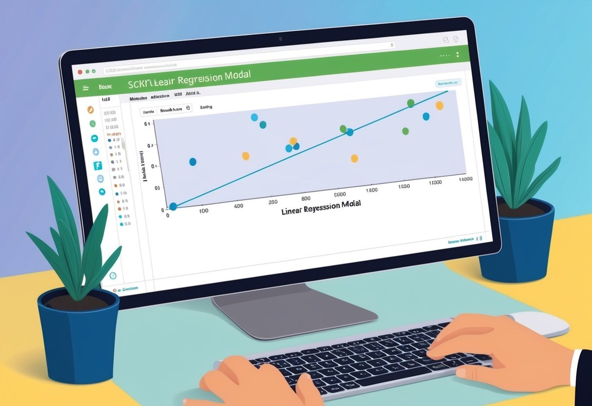
This approach involves plotting data points on a graph, drawing a line (the regression line) that best fits the points, and using this line to make predictions.
In the case of a simple linear regression, there is one independent variable, while multiple linear regression involves two or more. This method is based on the principle of minimizing the sum of the squared differences between observed and predicted values, known as the least squares method.
Techniques in linear regression can help in determining which features (or independent variables) significantly impact the dependent variable, thereby improving prediction accuracy.
Components of a Regression Equation
A regression equation is essential in representing the relationship between the independent and dependent variables.
In its simplest form, the equation is expressed as:
[ y = mx + c ]
Here, y represents the dependent variable or the predicted outcome, and x denotes the independent variable or the feature. The constant m is the slope of the line, showing how changes in the independent variable affect the dependent variable.
The intercept c is where the line crosses the y-axis, representing the value of y when x is zero.
In multiple linear regression, the equation becomes:
[ y = b_0 + b_1x_1 + b_2x_2 + ldots + b_nx_n ]
Where b_0 is the intercept, and each b_i represents the coefficient that measures the impact of each independent variable (x_i) on the dependent variable. Understanding these components is crucial for building effective regression models that can accurately predict outcomes.
Exploring the SciKit-Learn Library
SciKit-Learn is a popular Python library for machine learning. It is known for its easy-to-use tools, especially for supervised machine learning tasks like linear regression.
Installing SciKit-Learn
To get started with SciKit-Learn, Python must first be installed on the computer.
Use the Python package manager, pip, to install the library. Open the terminal or command prompt and enter:
pip install scikit-learn
This will download and install the latest version of SciKit-Learn.
The installation process is straightforward, making it accessible for beginners and experienced users.
It’s important to regularly update the library by using:
pip install --upgrade scikit-learn
This ensures access to the latest features and improvements.
Key Features of SciKit-Learn
SciKit-Learn offers a wide range of machine learning models, including linear regression, decision trees, and support vector machines. It is built on top of well-known Python libraries like NumPy and SciPy, ensuring swift numerical operations.
The library excels in providing tools for model selection and evaluation, such as cross-validation and grid search. These tools help refine and assess the performance of machine learning models.
Additionally, SciKit-Learn includes functions for data preprocessing, like feature scaling and normalization, which are crucial for effective model training.
It offers a consistent API, making it easier for users to switch between different models and tools within the library without much hassle.
Preparing the Dataset for Training
Preparing a dataset involves several important steps to ensure the model gets the best input for training. This process includes importing data using pandas and cleaning it for accurate analysis.
Importing Data with Pandas
Pandas is a powerful tool for data analysis in Python. It simplifies reading and manipulating datasets.
To start, datasets, often stored as CSV files, are loaded into a pandas DataFrame using the pd.read_csv() function.
For example, if the dataset is named data.csv, it can be imported with:
import pandas as pd

data = pd.read_csv('data.csv')
Once the data is in a DataFrame, it can be explored to understand its structure. Viewing the first few rows with data.head() gives insight into columns and their values. This step helps identify any issues in the data format, such as missing or incorrect entries, which are crucial for the next step.
Data Cleaning and Preprocessing
Data cleaning and preprocessing are essential to ensure the data quality before training.
Missing values can be handled by removing incomplete rows or filling them with mean or median values. For instance, data.dropna() removes rows with missing values, while data.fillna(data.mean()) fills them.
Standardizing data is also important, especially for numerical datasets. Applying techniques like normalization or scaling ensures that each feature contributes evenly to the model’s training.
Also, splitting the dataset into a training dataset and a testing dataset is crucial. Popular libraries like scikit-learn provide functions like train_test_split() to easily accomplish this task, ensuring the model’s performance is unbiased and accurate.
Visualizing Data to Gain Insights
Visualizing data helps in understanding patterns and relationships within datasets. Tools like Matplotlib and Seaborn provide powerful methods to create meaningful visualizations that aid in the analysis of data.
Creating Scatterplots with Matplotlib
Scatterplots are essential for visualizing the relationship between two variables. Matplotlib, a well-known library in Python, enables users to create these plots effortlessly.
It allows customization of markers, colors, and labels to highlight key points.
To create a scatterplot, one often starts with the pyplot module from Matplotlib. The basic function, plt.scatter(), plots the data points based on their x and y coordinates.
Users can further customize by adding titles using plt.title() and labels via plt.xlabel() and plt.ylabel(). These enhancements make the plot more informative.
Matplotlib also allows for adding grids, which can be toggled with plt.grid(). By using these features, users can create clear, informative scatterplots that reveal trends and correlations, making it easier to identify patterns in data.
Enhancing Visualization with Seaborn
Seaborn builds on Matplotlib by offering more sophisticated visualizations that are tailored for statistical data. It simplifies the process of creating attractive and informative graphics.
With functions like sns.scatterplot(), Seaborn can produce scatterplots with enhanced features. It supports additional styles and themes, making it easier to differentiate between groups in the data.
Users can also use hue to color-code different data points, which adds an extra layer of information to the visualization.
Seaborn’s integration with Pandas allows users to directly use DataFrame columns, making data visualization smoother. This ease of use helps in rapidly prototyping visualizations, allowing analysts to focus on insights rather than coding intricacies.
Splitting Data into Training and Test Sets
Dividing data into separate training and test sets is crucial in developing a machine learning model. It helps evaluate how well the model performs on unseen data. This process often involves the use of scikit-learn’s train_test_split function, with options to adjust random state and shuffle.
Using the train_test_split Function
The train_test_split function from scikit-learn is a straightforward way to divide datasets. This function helps split the data, typically with 70% for training and 30% for testing. Such a division allows the model to learn patterns from the training data and then test its accuracy on unseen data.
To use train_test_split, you need to import it from sklearn.model_selection. Here’s a basic example:
from sklearn.model_selection import train_test_split
X_train, X_test, y_train, y_test = train_test_split(data, target, test_size=0.3)
This code splits the features (data) and labels (target) into training and testing subsets. Adjust the test_size to change the split ratio.
Using this function helps ensure that the model evaluation is unbiased and reliable, as it allows the algorithm to work on data that it hasn’t been trained on.
Understanding the Importance of Random State and Shuffle
The random_state parameter in train_test_split ensures consistency in dataset splitting. Setting random_state to a fixed number, like 42, makes your results reproducible. This means every time you run the code, it will generate the same train-test split, making debugging and validation easier.
The shuffle parameter controls whether the data is shuffled before splitting. By default, shuffle is set to True.
Shuffling ensures that the data is mixed well, providing a more representative split of training and test data. When the data order affects the analysis, such as in time series, consider setting shuffle to False.
These options help control the randomness and reliability of the model evaluation process, contributing to more accurate machine learning results.
Building and Training the Linear Regression Model
Linear regression involves using a mathematical approach to model the relationship between a dependent variable and one or more independent variables. Understanding the LinearRegression class and knowing how to fit the model to a training set are key to implementing the model effectively.
Working with the LinearRegression Class
The LinearRegression class in SciKit Learn is vital for performing linear regression in Python. This class allows users to create a model that predicts a continuous outcome. It requires importing LinearRegression from sklearn.linear_model.
Core attributes of the class include coef_ and intercept_, which represent the slope and y-intercept of the line best fitting the data.
Users can also explore parameters like fit_intercept, which determines whether the intercept should be calculated. Setting this to True adjusts the model to fit data better by accounting for offsets along the y-axis.
Additionally, SciKit Learn features helpful methods such as fit(), predict(), and score().
The fit() method learns from the training data, while predict() enables future value predictions. Finally, score() measures how well the model performs using the R^2 metric.
Fitting the Model to the Training Data
Fitting the model involves splitting data into a training set and a test set using train_test_split from sklearn.model_selection. This split is crucial to ensure the model generalizes well to unseen data. Typically, 70-80% of data is used for training, while the rest is for testing.
The fit() method adjusts model parameters based on the training data by minimizing the error between predicted and actual values.
Once fitted, the model can predict outcomes using the predict() method. To evaluate, the score() method provides a performance measure, offering insights into prediction accuracy.
Adjustments to the model can be made through techniques like cross-validation for improved results.
Evaluating Model Performance
Evaluating the performance of a linear regression model is essential for understanding how well it can predict new data. Two key aspects to consider are interpreting the model’s coefficients and using various evaluation metrics.
Interpreting Coefficients and the Intercept
In a linear regression model, coefficients represent the relationship between each independent variable and the dependent variable. These values show how much the dependent variable changes with a one-unit change in the independent variable, keeping other variables constant.
The intercept is where the regression line crosses the y-axis.
For example, if a coefficient is 2.5, it means that for every one-unit increase in the predictor variable, the outcome variable increases by 2.5 units. Understanding these values can help explain how factors influence the outcome.
Utilizing Evaluation Metrics
Evaluation metrics are crucial for assessing prediction accuracy and error.
Common metrics include Mean Absolute Error (MAE), Mean Squared Error (MSE), and Root Mean Squared Error (RMSE).
MAE provides the average magnitude of errors in a set of predictions without considering their direction, making it easy to interpret.
MSE squares the errors before averaging, penalizing larger errors more than smaller ones.
RMSE takes the square root of MSE, bringing it back to the original unit of measurement, which can be more intuitive.
High precision and recall values indicate that the model accurately predicts both positive and negative outcomes, especially in binary classification tasks.
Accurate evaluation metrics offer a clearer picture of a model’s effectiveness.
Making Predictions with the Trained Model
Using a machine learning model to make predictions involves applying it to a set of data that wasn’t used during training. This helps in assessing how well the model performs on unseen data.
The focus here is on predicting values for the test set, which is a critical step for verifying model accuracy.
Predicting Values on Test Data
Once a model is trained using a training dataset, you can use it to predict outcomes on a separate test set.
For instance, if you are working with linear regression to predict housing prices, the model uses the test data to provide predicted prices based on given features like location or size.
This is crucial for evaluating the model’s performance.
The test set typically consists of about 20-30% of the overall dataset, ensuring it reflects real-world data scenarios.
In Python, the predict() method from libraries like Scikit-Learn facilitates this process. Input the test features to retrieve predictions, which should be checked against true values to measure accuracy.
Understanding the Output
The predictions generated are numerical estimates derived from the given features of the test data. For housing prices, this means the predicted values correspond to expected prices, which require validation against real prices from the test set.
Tools like Mean Squared Error (MSE) help in quantifying the accuracy of these predictions.
Understanding the output helps in identifying any patterns or significant deviations in the predicted values.
Evaluating these results could lead to refining models for better accuracy.
Moreover, visual aids like scatter plots of predicted versus actual values can provide a clearer picture of the model’s performance. This approach ensures thorough analysis and continuous learning.
Improving the Model with Hyperparameter Tuning
Hyperparameter tuning can significantly enhance the performance of a linear regression model by adjusting the parameters that influence learning. This approach helps in managing underfitting and overfitting and exploring alternative regression models for better accuracy.
Dealing with Underfitting and Overfitting
Underfitting occurs when a model is too simple, failing to capture the underlying trend of the data. This can be mitigated by adding more features or by choosing a more suitable model complexity.
Overfitting happens when a model learns the noise in the data as if it were true patterns, which can be controlled using regularization techniques like Lasso (L1) or Ridge (L2). Regularization helps to penalize large coefficients, thereby reducing model complexity.
Tuning the hyperparameters, such as the regularization strength in Lasso regression, is crucial.
Using methods like GridSearchCV, one can systematically test different parameters to find the best configuration. Cross-validation further aids in ensuring that the model works well on unseen data.
Exploring Alternative Regression Models
While linear regression is a fundamental tool for regression tasks, exploring alternatives like logistic regression or polynomial regression can sometimes yield better results.
These models can capture more complex relationships as compared to a simple regression line generated by ordinary least squares.
Logistic regression, though primarily used for classification tasks, can handle binary outcomes effectively in a regression context.
Boosting methods or support vector machines (SVMs) are advanced options that can also be explored if basic models do not suffice.
Different models have different sets of hyperparameters that can be tuned for improved performance. By carefully selecting models and adjusting their hyperparameters, one can enhance the predictive power and reliability of the regression analysis.
Integrating the Model into a Python Script

Integrating a machine learning model into a Python script involves creating functions for making predictions and handling model files. This process ensures that models can be reused and shared easily, especially in environments like Jupyter Notebooks or platforms like GitHub.
Writing a Python Function for Prediction
When integrating a model, writing a dedicated function for prediction is crucial. This function should take input features and return the predicted output.
Implementing it in a Python script makes the prediction process straightforward and accessible.
The function can be designed to accept input as a list or a NumPy array. Inside the function, necessary preprocessing of input data should be done to match the model’s requirements.
This may include scaling, encoding categorical variables, or handling missing values. Once preprocessing is complete, the model’s predict method can be called to generate predictions.
This setup allows seamless integration within a Jupyter Notebook, where users can input new data instances and instantly get predictions.
Keeping the prediction function modular helps maintain code clarity and makes collaborating on projects in environments like GitHub more efficient.
Saving and Loading Models with Joblib
Using Joblib to save and load machine learning models is essential for efficient workflows. Joblib is a Python library for efficient job management and provides utilities for saving complex data structures like trained models.
To save a model, the script uses joblib.dump(model, 'model_filename.pkl'). This saves the model to a file, capturing the model’s current state along with learned parameters.
Loading the model later is just as simple: model = joblib.load('model_filename.pkl').
This approach ensures models can be shared or deployed without retraining, saving time and computational resources.
This capability is particularly beneficial in collaborative projects stored on GitHub, where consistent access to the trained model is necessary for development and testing.
Hands-On Practice: Predicting Housing Prices
Predicting housing prices involves using real data and considering various challenges. Key points include using actual housing data and understanding the obstacles in predictive modeling.
Using Real Housing Data
Using actual housing data is crucial for accurate predictions. The data usually includes information such as house age, number of rooms, income levels, and population. These factors are key inputs for the model.
When using Scikit-learn, the data is split into training and testing sets. This helps in evaluating the model’s performance.
Train-test split function is a common method used in predictive modeling. The training set enables the model to learn, while the test set evaluates its predictive accuracy.
Linear regression is widely used for this task due to its simplicity and effectiveness. This method aims to fit a line that best describes the relationship between inputs and housing prices. Understanding these relationships helps in making informed predictions.
Challenges and Considerations
Working with housing data comes with challenges. One major challenge is handling missing or incomplete data, which can skew results. Data preprocessing is essential to clean and prepare data for analysis.
Data interpretation is another critical factor. Variable importance and their impact on prices need careful consideration.
Overfitting is a common issue, where the model works well on training data but poorly on unseen data. Techniques like Lasso regression can mitigate this by simplifying the model.
Choosing the right features for prediction is crucial. Including irrelevant features can reduce model accuracy.
Evaluating and fine-tuning the model regularly ensures robustness and improves its predictive power. These considerations are vital for accurate and reliable housing price predictions.
Appendix: Additional Resources and References
In learning about linear regression and splitting datasets, practical resources and community-driven examples are essential. This section introduces insightful materials for statistical learning and useful code repositories.
Further Reading on Statistical Learning
For those interested in a deeper dive into statistics and supervised learning, several resources stand out.
The scikit-learn documentation provides an extensive overview of linear models and how to implement them in data science projects. It covers concepts like regularization and different types of regression techniques.
Another useful resource is Linear Regressions and Split Datasets Using Sklearn. This article demonstrates how to use pandas dataframes and sklearn to handle data preparation. It is particularly helpful for beginners who need step-by-step guidance on dataset splitting.
Code Repositories and Datasets
GitHub is a valuable platform for accessing practical code examples and datasets.
The repository Train-Test Split and Cross-Validation in Python includes a Jupyter Notebook that guides users through implementing these essential techniques in data science. It contains explanations, code, and visualizations to support learning.
When working with pandas dataframes and sklearn, exploring datasets available via sklearn can be beneficial. These datasets are excellent for practicing and refining skills, offering opportunities to perform regression analysis and understand features in real-world data scenarios.
Frequently Asked Questions
Linear regression is a fundamental concept in machine learning. This section addresses common questions about using scikit-learn to perform a train/test split, the role of the ‘random_state’ parameter, and challenges in implementation.
How do you perform a train/test split for a linear regression model using scikit-learn?
Using scikit-learn to perform a train/test split involves importing the train_test_split function from sklearn.model_selection.
Data is divided into training and testing sets. This helps evaluate the linear regression model. For detailed instructions, check resources that explain how to split datasets.
What is the purpose of stratifying the train/test split in scikit-learn?
Stratifying during a train/test split ensures that each set maintains the same class distribution as the full dataset. This is crucial when dealing with imbalanced data, as it helps in achieving reliable performance metrics.
How does the ‘random_state’ parameter affect the train/test split in scikit-learn?
The ‘random_state’ parameter ensures that the train/test split is reproducible.
By setting a specific value, the same split will occur each time, allowing for consistent evaluation across different runs or experiments.
Is it necessary to split the dataset into training and testing sets when performing linear regression?
Splitting data into training and testing sets is critical for a valid performance assessment. It helps in understanding how well the linear regression model generalizes to unseen data.
Without this split, there’s a risk of overfitting the model to the training data.
Can you explain the process of linear regression within scikit-learn?
Linear regression in scikit-learn involves using the LinearRegression class.
The typical process includes fitting the model with data, predicting outcomes, and evaluating the model’s performance. More information on linear regression is available through tutorials.
What are the challenges one might face when implementing linear regression?
Implementing linear regression can present several challenges. These may include handling multicollinearity, ensuring data is clean and formatted correctly, and dealing with outliers.
Proper preprocessing and understanding data characteristics are essential to address these challenges effectively.