Categories
Uncategorized

Azure Data Studio Diagram: A Comprehensive Guide to Visual Database Design

Understanding Azure Data Studio

Azure Data Studio offers a range of features that make it a versatile tool for data professionals. It supports multiple operating systems, including Windows, Linux, and macOS.

Users can benefit from its capabilities in database development and management, with an emphasis on ease of use and integration with other tools.

Overview of Features

Azure Data Studio provides several key features tailored for database administrators and developers. It supports various SQL-based workloads while offering a modern and efficient coding environment.

The software comes equipped with IntelliSense, helping users write queries more effectively. Built-in features like dashboards and customizable extensions enhance productivity and user experience, making it a valuable asset for managing large volumes of data.

Users can benefit from its ability to support multiple database connections, facilitating the management of different databases simultaneously. Its cross-platform capability allows users to operate seamlessly on Windows, Linux, and macOS.

This flexibility makes Azure Data Studio a reliable choice for professionals looking to optimize their data management processes. Extensions further enhance functionality, with several available to add specific features or improve performance.

Navigating the Object Explorer

The Object Explorer in Azure Data Studio is a pivotal tool for managing database components. It provides a hierarchical view of database objects, allowing users to efficiently browse through tables, views, procedures, and more.

This feature simplifies database management tasks by providing a clear and organized view of the data structure.

Users can interact directly with database objects through the Object Explorer, enabling them to perform tasks such as editing tables or running queries with ease. The interface supports custom filtering, which helps in focusing on specific objects of interest.

Intuitive design ensures that users can quickly access necessary information without navigating through complex menus.

Code Snippets and Source Control Integration

Azure Data Studio enhances productivity with code snippets, which allow users to quickly insert frequently used code blocks. This feature reduces typing overhead and ensures consistency across different scripts.

Users can create custom snippets tailored to their specific coding patterns, further streamlining the development process.

Source control integration, such as with Git, provides robust version management for scripts and projects. This integration helps users track changes, maintain version history, and collaborate with team members effectively.

Source control tools are accessible within the interface, enabling easier management of repositories alongside database development work.

Integrated Terminal Usage

The integrated terminal in Azure Data Studio offers seamless command-line access. Users can switch between coding and executing terminal commands without leaving the application.

This integration supports various terminals, like Bash on Linux and macOS, and PowerShell on Windows, catering to diverse user preferences.

This terminal feature proves valuable for executing administrative tasks, such as database backups, directly from within Azure Data Studio.

Advanced users benefit from scripting capabilities within the integrated terminal, which enhances overall efficiency by reducing the need to switch between different applications while performing complex data operations.

Working with Database Diagrams in Azure Data Studio

Azure Data Studio provides tools to create and edit database diagrams effectively. Users can visualize relationships between tables, making database design more intuitive. The platform supports creating new diagrams and modifying existing databases to fit evolving needs.

Creating Database Diagrams

To start with Azure Data Studio, users can easily create database diagrams. After launching the application and connecting to a SQL Server instance, they should navigate to the Object Explorer pane, choose the desired database, and start a new query window.

While Azure Data Studio doesn’t inherently support schema diagramming, users can explore external tools like DBeaver, which offers a View Diagram feature for databases.

Creating these diagrams often involves understanding the entities and relationships within the database—commonly referred to as ER diagrams. These graphical representations help in ensuring that tables are linked correctly and that data constraints are maintained across tables.

Editing and Modifying Tables

Azure Data Studio allows modifications to existing tables to ensure the database scheme remains adaptable to changes. Users can edit tables directly within the SQL query editor to add, remove, or modify columns as necessary.

These updates facilitate the evolving data requirements and dynamics of modern applications.

The use of keyboard shortcuts such as Ctrl+N for new entities and Ctrl+Z to undo changes can streamline the editing process. This ease of use plays a crucial role in making sure that database modifications are executed smoothly without disrupting existing services.

Visualizing Table Relationships

Visualizing table relationships is crucial in database design to ensure integrity and functionality. While Azure Data Studio might not support advanced visualization natively, it provides foundational tools for basic insights.

Users can understand connections by analyzing foreign keys and dependencies between tables.

For comprehensive visualization, external plugins or tools like DBeaver can be integrated. These options allow users to view detailed relationship maps that depict the entire database structure, making it easier to optimize and maintain healthy database systems.

Such visual tools contribute significantly to clear data modeling and ER diagram refinement.

Managing SQL Schemas and Data

In Azure Data Studio, effective management of SQL schemas and data involves aspects like executing SQL queries, visualizing schema structures, and establishing best practices for handling sample data. These components are crucial for ensuring database integrity, performance, and ease of use.

Executing SQL Queries

Azure Data Studio provides a robust environment for executing SQL queries, which allows users to interact directly with their database. Users can write and run queries to retrieve or manipulate data using familiar T-SQL syntax. The query editor in Azure Data Studio supports key features such as syntax highlighting, smart IntelliSense, and code snippets, helping to streamline the process.

Save frequently used queries in the editor for quick access. It’s also possible to format queries for better readability and organize results into tables, making it easier to interpret the data.

Configurable connection options ensure secure and efficient execution of queries across different environments.

Schema Visualization and Management

Schema visualization is an essential feature that provides a graphical view of database structures. Using Azure Data Studio, users can visually represent tables, relationships, indexes, and constraints through schema diagrams. This capability enhances the understanding of complex database relationships.

To get started, create or open a database instance in Azure Data Studio. Use tools for designing and managing schemas effectively.

Schema changes can be made directly within the tool, including adding new tables, modifying columns, or updating relationships.

For more detailed guidance, users can explore resources on schema visualization in Azure Data Studio.

Sample Data and Best Practices

Working with sample data is critical when developing or testing database applications. Azure Data Studio allows you to manage sample data efficiently, helping to simulate real-world scenarios.

Incorporate best practices, such as backing up data before making changes and using transaction controls to maintain data integrity.

It’s important to validate changes with sample datasets before applying them to production environments. Incorporate various data types, constraints, and indexes when working with samples to reflect true operational scenarios.

Adopting these best practices ensures seamless transitions from development to production, minimizing errors and optimizing data management.

Database Objects and Design Concepts
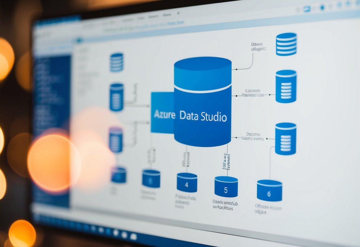
A diagram in Azure Data Studio depicting database objects and design concepts

Database design involves structuring databases efficiently. This requires careful consideration of keys and relationships, choosing appropriate data types for columns, and implementing indexes and constraints to optimize performance.

Understanding Keys and Relationships

Keys are fundamental to database design. They ensure data integrity and create links between tables. A primary key uniquely identifies each record within a table. Usually, it is a single column but can be a combination of columns.

Relationships establish how tables relate. These are often built using foreign keys, which reference a primary key in another table. This setup helps maintain consistent data and facilitates complex queries.

In Azure Data Studio, using the interface to visualize relationships can help users understand how different tables are interlinked.

Defining Columns and Data Types

Choosing the correct data types for columns is crucial. Data types determine what kind of data can be stored. Common types include integers, decimals, and strings such as nvarchar, which stores variable-length text.

The design of columns should reflect their purpose. For example, a date of birth column should use a date type, while a column for names might use nvarchar.

Properly defined columns not only enhance efficiency but also prevent potential errors during data entry.

Implementing Indexes and Constraints

Indexes are used to improve query speed. They allow quicker data retrieval by creating an ordered structure based on one or several columns. While powerful, too many indexes can lead to slower write operations.

Constraints enforce rules on data in tables. Examples include unique constraints that ensure all values in a column are different and check constraints that validate the data based on specific conditions.

These features help maintain data integrity by preventing invalid data entries.

Efficiently implementing indexes and constraints in Azure Data Studio requires understanding their impact on performance and storage. Adding the right constraints ensures data remains consistent and reliable without adverse effects on the overall system efficiency.

Generating Entity-Relationship Diagrams

An open laptop displaying an Entity-Relationship Diagram in Azure Data Studio, with various tables and connections

Creating Entity-Relationship (ER) Diagrams in Azure Data Studio helps visualize the structure of databases. These diagrams illustrate tables, columns, and relationships, making it easier to manage and document databases effectively.

Generate ER Diagrams from Existing Databases

To start generating ER diagrams in Azure Data Studio, users can connect to their existing databases. After connecting, they can select specific tables or entities they want to include. This helps in understanding how different database elements interconnect.

Tools like the Schema Visualization plugin assist in this process by providing visual insights into database structures.

Users can configure the plugin to highlight key relationships and attributes. This enables data analysts to detect potential design issues before implementing changes.

Users interested in learning more about using this plugin can find a detailed guide on how to generate an ER diagram in Azure Data Studio.

Documenting Database Structures

ER diagrams play a vital role in documenting relational databases. They graphically represent entities, attributes, and their interconnections, which aids in maintaining clear documentation.

This visual documentation is crucial for onboarding new team members and collaborating with others.

Creating these diagrams ensures that the database structure is well-documented, enhancing communication among team members. They serve as a reference point during database development, providing clarity on complex relationships.

Users can create and maintain these diagrams using tools available in Azure Data Studio, making them an integral part of database management practices. Learn more about the benefits of documenting databases with ER diagrams at Creating Schema Diagrams in Azure Data Studio.

Azure Data Studio and SQL Server Integration

An open laptop displaying Azure Data Studio with a connected SQL Server Integration Services diagram on the screen

Azure Data Studio offers seamless integration with SQL Server, making it a versatile tool for database management and development tasks. Users can efficiently connect to, manage, and migrate SQL Server databases, enhancing their workflow and productivity.

Connecting to Various SQL Server Types

Azure Data Studio supports a range of SQL Server types, providing flexibility for users. It connects to traditional SQL Server instances, Azure SQL Database, and Azure SQL Managed Instance. This allows users to manage on-premises and cloud-based databases with ease.

The integration includes features like a customizable dashboard and rich T-SQL editing capabilities.

Compatibility with the Analytics Platform System (APS) further enhances its utility in more complex environments. Users have the ability to connect and manage workloads across different platforms.

The tool is designed to support professionals in diverse database scenarios, making it an excellent choice for those using various SQL Server types in their operations.

Migrating from SSMS to Azure Data Studio

Transitioning from SQL Server Management Studio (SSMS) to Azure Data Studio can be a straightforward process for most users. Azure Data Studio’s interface is user-friendly and offers extensions that enhance functionality, like the SQL Server Import extension, allowing for smooth data migration.

Many features familiar to SSMS users are present, such as query editor tools and integrated terminal support.

The inclusion of SQL Server Migration Extensions simplifies moving databases from SSMS, easing the adaptation process.

By supporting core SQL Server functions, Azure Data Studio reduces the learning curve for users migrating from SSMS, making it a valuable tool for those looking to modernize their database management setup. With community support growing, users can find ample resources for troubleshooting and optimizing their workflows in this environment.

Frequently Asked Questions

A person using Azure Data Studio, surrounded by FAQ documents and diagrams

Azure Data Studio offers various tools for visualizing and managing database schemas.

Users can create ER diagrams, compare schemas, and manage databases with ease.

How can I generate an ER diagram using Azure Data Studio?

To generate an ER diagram, launch Azure Data Studio and open your database.

Use available tools and extensions, if any, to visualize the database structure.

Is there an extension for database diagram visualizations in Azure Data Studio?

Azure Data Studio supports extensions that may assist in database visualization.

Check the extensions marketplace for relevant tools that enhance diagram creation.

What are the steps to visualize a database schema in Azure Data Studio?

Begin by opening Azure Data Studio.

Navigate to your database, and use the schema diagram feature to view relationships between tables.

Specific steps vary based on the version and installed extensions.

Can Azure Data Studio be used for schema comparison, and how?

Azure Data Studio can be used for schema comparison with the right tools.

Look for extensions that allow this feature, enabling side-by-side schema analysis.

How to create and manage a new database within Azure Data Studio on a Mac?

On a Mac, open Azure Data Studio and use the built-in tools to create a new database.

Follow prompts to set up tables and schema as needed.

What methods are available for viewing a table diagram in Azure Data Studio similar to SQL Server Management Studio?

In contrast to SQL Server Management Studio, Azure Data Studio does not offer native support for table diagrams.

External tools such as DBeaver may be used for this purpose to visualize diagrams effectively.

Categories
Uncategorized

Learning T-SQL – Table Creation Simplified Guide

Understanding T-SQL and SQL Server Basics

Learning T-SQL and SQL Server basics lays the foundation for strong database management skills. Key elements include understanding the differences between SQL and T-SQL and how to use SQL Server Management Studio (SSMS) effectively.

Defining SQL and T-SQL

Structured Query Language (SQL) is the standard language for interacting with databases. It allows users to create, modify, and manage data easily. SQL is crucial for tasks like querying databases, inserting data, and updating records.

Transact-SQL (T-SQL) is an extension of SQL used by SQL Server. It includes additional features such as procedural programming, local variables, and support for functions like IF statements and loops. These enhancements make T-SQL powerful for complex database operations and efficient data management within SQL Server environments.

Understanding both languages is vital. SQL forms the backbone of database manipulation, while T-SQL provides advanced tools for more sophisticated tasks. Learning their differences ensures effective use of SQL Server capabilities.

Exploring SQL Server Management Studio (SSMS)

SQL Server Management Studio (SSMS) is an essential tool for managing SQL Server databases. It offers a user-friendly interface to interact with databases, run queries, and configure database settings.

In SSMS, users can create and modify database objects, execute T-SQL scripts, and perform administrative tasks like backups. Features such as the query editor and graphical tools enhance database management and provide a comprehensive view of SQL Server infrastructure.

SSMS supports T-SQL development and simplifies troubleshooting with debugging capabilities. Its visual designers help users navigate SQL Server environments, making it easier to handle the complexities of database operations. Being familiar with SSMS allows users to harness the full potential of SQL Server, improving productivity and efficiency in daily tasks.

Setting up Your SQL Server Environment

Setting up an SQL Server environment involves creating a new database and deciding on a default schema. These steps are crucial for organizing data and ensuring smooth operations in SQL Server.

Creating a New Database

When creating a new database, the SQL command CREATE DATABASE is used. This command requires a unique database_name as the primary argument. For instance, to create a database named “SalesData,” you would execute CREATE DATABASE SalesData. This command informs SQL Server to allocate space for the new database and establishes default settings.

Once the database is created, it’s important to configure settings such as file locations and sizes. This can be done by specifying options like FILENAME or MAXSIZE. These settings help in managing storage and performance. By organizing files properly, users can optimize database access and maintenance.

Understanding Default Schema

In SQL Server, the default schema is significant when users create new database objects like tables or views. By default, many objects are created within the dbo (database owner) schema if not specified otherwise. This is manageable for many applications, but selecting appropriate schemas is encouraged for complex environments.

Having a defined schema helps categorize objects based on their roles or applications. For example, organizing schema by department (sales, hr, finance) ensures clear data segregation. This approach minimizes conflicts and aids in maintaining a clean database structure, facilitating easier management and security configuration.

Using commands like ALTER USER or CREATE SCHEMA, users can specify or change the default schema, ensuring that new objects integrate appropriately into the existing structure.

Designing Robust Database Tables

Designing robust database tables requires careful planning to ensure data integrity and organizational efficiency. Key aspects of this process include determining the table structure and establishing effective naming conventions, as well as using schemas to efficiently organize data.

Planning Table Structure and Naming Conventions

The table structure is critical to how data is stored and accessed. When creating a database table, defining clear and logical columns is essential. Column names should accurately describe the data they hold, making it easier for others to understand their purpose. Choosing appropriate data types for each column helps maintain data integrity and optimize storage.

Naming conventions play a crucial role in database management. Consistency in naming conventions makes database tables more readable and maintainable. For example, using a standard prefix or suffix for all table names can quickly inform users about the content or nature of each table. Naming conventions should be agreed upon by the team and documented for future reference.

Leveraging Schemas for Organizational Efficiency

Schemas are powerful tools in database design for segmenting and organizing data logically. By using schemas, developers can group related tables together, improving both structure and retrieval times. This organization allows for more efficient data management and can help prevent naming conflicts.

Schemas also provide a means to enforce security and permissions by controlling who can access specific groups of tables. In many systems, schemas are used to separate different modules or features of an application, which simplifies development and maintenance. Designing a thoughtful schema structure from the beginning contributes to a scalable and manageable database architecture.

Fundamentals of Data Types and Columns in T-SQL

In T-SQL, choosing the right data types and defining columns properly ensures efficient database management. It affects how data is stored, accessed, and processed.

Choosing the Right Data Types

Selecting the correct data type is crucial for optimizing storage and performance. Common data types include integers (int), characters (char, varchar), datetime, decimal, and money.

For numeric data, use int for whole numbers or decimal for precise values. Text data can be stored as char for fixed length or varchar for variable length. Datetime is used for date and time values, while money handles financial data.

Consider storage size and application needs. A smaller data type reduces storage space, but ensure it meets data requirements.

Defining Columns and Nullability

Defining columns involves choosing their names and data types. It’s important to set whether a column can hold a null value or not.

A column with null allows missing or unknown data, providing flexibility. When a column is defined as not null, every entry must have a value, ensuring data completeness.

When designing a table, use not null for columns requiring mandatory data. For optional data, null can be used. Understanding column nullability affects data integrity and application logic.

Mastering the CREATE TABLE Statement

Creating tables in SQL involves understanding the syntax and applying constraints to ensure data integrity. It’s important to craft a functional table structure and incorporate necessary elements like constraints and indexes. This ensures the table’s seamless performance and reliability.

Crafting the Basic Create Table Syntax

To start with the SQL CREATE TABLE statement, one must know the essential components involved. A basic CREATE TABLE involves defining the table name, followed by specifying columns and their data types. For example:

CREATE TABLE Employees (
    EmployeeID INT,
    Name VARCHAR(50),
    HireDate DATE
);

This syntax sets up a table named “Employees” with three columns. Each column has a specific data type – INT for EmployeeID, VARCHAR for Name, and DATE for HireDate. By structuring columns correctly, users ensure that data is accurately stored and accessible.

Incorporating Table Constraints and Indexes

In an SQL CREATE TABLE statement, constraints such as PRIMARY KEY, FOREIGN KEY, UNIQUE, and NOT NULL maintain data accuracy and relationships. For example:

CREATE TABLE Employees (
    EmployeeID INT PRIMARY KEY,
    Name VARCHAR(50) NOT NULL,
    DepartmentID INT,
    FOREIGN KEY (DepartmentID) REFERENCES Departments(DepartmentID)
);

This example uses a PRIMARY KEY to uniquely identify each record. A FOREIGN KEY ensures that every DepartmentID matches a valid department entry. Constraints like NOT NULL prevent empty fields, adding data reliability.

Indexes enhance query performance. While they aren’t specified within the CREATE TABLE syntax, planning their inclusion is key. Indexing frequently queried columns decreases data retrieval time, optimizing table functionality.

Implementing Constraints and Keys

In T-SQL, implementing constraints and keys is essential for maintaining data accuracy and consistency within a database. This involves using primary keys to uniquely identify records, and foreign keys to uphold relationships between tables.

Working with Primary Keys

A primary key serves as a unique identifier for each record in a table, ensuring no duplicate rows exist. This key is crucial for database normalization and efficient data retrieval. A primary key constraint combines the NOT NULL and UNIQUE constraints, meaning every value must be unique and not missing.

Tables in T-SQL often utilize an integer datatype for primary keys due to its efficiency. Implementing primary keys not only helps with data integrity but also aids in referential integrity, which connects related tables. Without a unique primary key, maintaining a reliable database structure becomes challenging. Understanding primary keys is fundamental in learning T-SQL.

Ensuring Data Integrity with Foreign Keys and Checks

Foreign keys ensure referential integrity by linking tables and maintaining consistency across related data. When a table uses a foreign key, it references a primary key from another table, establishing a parent-child relationship. This means updates or deletions to the parent data will reflect in the child, maintaining consistent relationships.

The CHECK constraint is another tool used to define rules for the data in a column, such as ensuring a column only accepts positive numbers. Combining these constraints helps preserve data integrity and prevents invalid data from entering the system. They are crucial for anyone learning how to implement constraints and keys effectively in T-SQL.

Inserting and Managing Data

Inserting and managing data in T-SQL involves executing specific commands to handle entries in a database. Understanding how to use the INSERT INTO and UPDATE statements is crucial for effective data management.

Performing INSERT INTO Operations

The INSERT INTO command is essential for adding new records to a table. This statement ensures that data is input directly into specified columns. A typical INSERT INTO operation requires naming the table and listing columns where the data will exist.

Example:

INSERT INTO Employees (Name, Position, Salary) 
VALUES ('John Doe', 'Developer', 70000);

For multiple entries, the query can include several sets of values. Using the SELECT statement is an efficient way to insert data from one table into another. This method copies rows between tables, maintaining structure and relationships.

Example:

INSERT INTO NewEmployees (Name, Position, Salary) 
SELECT Name, Position, Salary FROM OldEmployees;
```### Updating Data with the UPDATE Statement

Updating existing entries in a table uses the `UPDATE` statement. This function changes data within the specified columns. 

It's important to use the `WHERE` clause to target specific records. Without it, all rows get updated, which might lead to errors. 

*Example:*

```sql
UPDATE Employees 
SET Salary = 75000
WHERE Name = 'John Doe';

This statement adjusts the salary only for John Doe’s entry.

To confirm updates, implementing a SELECT statement post-update helps verify that the right adjustments have occurred.

Efficient querying ensures that data integrity remains intact during these operations.

Utilizing SQL Functions and Expressions

T-SQL provides powerful tools for managing data. Key elements such as functions and expressions enhance data handling.

They allow for efficient data manipulation, column definition, and data entry, helping ensure attributes like data types and unique values are correctly implemented.

Leveraging Functions for Data Manipulation

SQL functions play a vital role in manipulating data efficiently. Functions like SYSDATETIME() and CURRENT_TIMESTAMP automatically generate date and time values when rows are inserted. This is helpful in maintaining accurate records without manual input.

Another important function is IDENTITY which generates unique numbers for each row in a table. This is especially useful for primary keys, ensuring that each row can be uniquely identified.

Data types and conversions are essential when working with functions.

Ensuring data is stored with the appropriate data type, SQL conversion functions like CAST or CONVERT can format data as needed. They ensure compatibility and accuracy across databases.

Using Expressions in Data Entry

Expressions in SQL allow for calculated data entry and default values.

For example, a DEFAULT expression can auto-fill a column with a specific value if none is provided. This ensures consistency and complete data sets.

Expressions can also enforce unique values by using unique constraints and conditional logic during data entry. This prevents duplicate data entries, maintaining data integrity across the database.

Column definitions also use expressions to specify data attributes, like NOT NULL to ensure necessary fields are never empty. This improves data completeness and reliability, essential for any robust database system.

Managing Database and Table Permissions

Managing permissions in a database involves determining who can access or modify data. This is important for maintaining security and data integrity.

Assigning roles and understanding who owns the database help in setting clear access controls.

Assigning Roles and Permissions

Assigning roles is crucial for defining access levels within a database. Each role can have specific permissions, such as the ability to read, write, or modify data tables.

Permissions are generally granted using T-SQL commands like GRANT and REVOKE.

Roles: Common roles include admin, user, and viewer. An admin can manage other roles and permissions, while a user might only add or modify existing data. A viewer could only read data without making changes.

Permissions: These must be tailored to each user’s needs. Access can be specified at multiple levels, such as at the database level or in relation to specific tables or schemas.

For example, giving a user permissions to SELECT from a table without allowing INSERT or DELETE.

Understanding Database Ownership

Database ownership determines who has ultimate control over all aspects of a database. The database owner typically has full permissions and usually manages user access and roles.

Ownership is often assigned at the database creation stage and involves responsibilities like maintaining database integrity and security.

Database Owner: An individual or role designated as the owner has unique rights. They can transfer ownership, alter database settings, and override permissions.

Schema Names and Permissions: Schemas group database objects such as tables, views, and functions under a distinct namespace.

By controlling schema permissions, one can organize who accesses specific parts of the database. Using schema names allows for easier management of tables with similar functions across databases, providing clear organization within the database_name and schema_name.

Advanced Table Options in T-SQL

T-SQL allows for advanced table management options that can significantly enhance database operations. In the following sections, you will learn about using temporary tables, transaction processing, and the importance of indexing.

Working with Temporary Tables

Temporary tables play a key role in T-SQL for managing large datasets or intermediate results without altering the original data. They are created in the system database tempdb, making them ideal for short-term operations.

Temporary tables can be defined with the CREATE TABLE statement. The table names typically start with a # to distinguish them.

When using temporary tables, data integrity and isolation must be maintained. They are automatically dropped when the user session ends, reducing the need for manual cleanup. This makes them efficient for testing and debugging.

Temporary tables provide flexibility, allowing changes and experiments without affecting the existing tables. Consider these when managing complex queries or when storing data temporarily is beneficial for the task.

Diving into Transaction Processing and Indexing

Transaction processing is essential in T-SQL for maintaining data consistency and integrity, especially during multiple data operations.

Transactions are initiated using BEGIN TRANSACTION. This ensures that a group of operations is completed successfully or not at all, thanks to COMMIT or ROLLBACK commands.

Indexing in T-SQL allows faster retrieval of rows in a table by creating a data structure that the database can search efficiently.

Choosing the right columns to index can dramatically improve query performance.

Indexes can be created using the CREATE INDEX command on existing tables. However, over-indexing may slow down write operations due to the additional maintenance required.

Balancing between transaction processing and indexing is crucial in optimizing database performance and reliability. Proper indexing strategies not only improve speed but also aid in maintaining a robust data management system.

Exploring Scalability and Performance

A computer screen displaying T-SQL code for creating tables, with a focus on scalability and performance

Understanding how to improve scalability and performance is essential when working with T-SQL. This involves optimizing query execution and maintaining consistent database performance, crucial for handling large data sets and complex operations efficiently.

Optimizing SQL Queries

Optimizing SQL queries is vital for efficient database management. Reducing query execution time can significantly enhance the user experience and resource utilization.

Techniques such as indexing and query refactoring play a crucial role in performance improvement.

Indexing helps in quickly locating data within tables, especially on large datasets. Refactoring involves rewriting queries for better execution plans.

Using execution plans to identify bottlenecks in queries allows for targeted optimizations.

In environments like the Azure SQL Database, monitoring query performance is straightforward due to built-in tools.

Query optimization can leverage SQL Server’s in-memory capabilities, reducing latency and improving throughput.

Maintaining Database Performance

Maintaining database performance involves regular monitoring and adjustments to settings and configurations.

It’s essential to manage resources effectively, especially when dealing with Azure SQL Managed Instance, which offers features for scalability.

Routine checks on disk usage, memory allocation, and CPU usage can prevent performance degradation.

Keeping an eye on workload patterns and adjusting resources accordingly help maintain optimal performance.

Utilizing features of the Analytics Platform System can enhance data processing capabilities, supporting scalability for large-scale operations.

Consistently updating and maintaining indexes, adjusting database settings, and performing database tuning tasks are key practices for maintaining a high-performance database environment.

Frequently Asked Questions

A person typing on a computer, creating a table in a database using T-SQL

This section addresses common questions about creating tables using T-SQL, including how to set up primary and foreign keys, the syntax for table creation, and best practices for naming. The examples provided will help in understanding and applying these concepts practically.

How do I create a table in T-SQL with a primary key?

To create a table with a primary key, use the CREATE TABLE statement and define the primary key with the PRIMARY KEY keyword. This ensures that the column specified uniquely identifies each record in the table.

What is the syntax for creating a new table using T-SQL?

The basic syntax for creating a table in T-SQL is:

CREATE TABLE table_name (
    column_name1 data_type1 constraints,
    column_name2 data_type2 constraints,
    ...
    PRIMARY KEY (column_name)
);

This statement outlines the table’s structure, including column names, data types, and any constraints.

Can you show an example of using CREATE TABLE AS SELECT in SQL Server?

In SQL Server, you can’t directly use CREATE TABLE AS SELECT like other SQL variants. Instead, you’d use SELECT INTO to create a new table from an existing table’s data:

SELECT *
INTO new_table_name
FROM existing_table_name
WHERE condition;

How to define foreign keys when creating a table in T-SQL?

To define a foreign key, include the FOREIGN KEY constraint in the CREATE TABLE statement:

FOREIGN KEY (column_name) REFERENCES parent_table(parent_column)

This links the table to another, enforcing referential integrity.

What are the best practices for naming columns and tables in T-SQL?

Names should be descriptive and follow a consistent format. Avoid using reserved SQL keywords.

Use underscores to separate words in names for readability, like user_id or order_number.

How do you add constraints during table creation in T-SQL?

Constraints like NOT NULL, UNIQUE, CHECK, PRIMARY KEY, and FOREIGN KEY are added directly in the CREATE TABLE statement.

For example:

CREATE TABLE example (
    id INT PRIMARY KEY,
    name VARCHAR(50) NOT NULL,
    age INT CHECK (age >= 0)
);

Constraints ensure data integrity and control what data can be entered into the table.

Categories
SQL

Filtering and Conditional Operations: Your Guide to Efficient Data Processing

Diving into the world of Filtering and Conditional Operations, you’ll soon discover that these concepts form the backbone of effective data management. Whether you’re dealing with an extensive sample database or a smaller set of structured information, understanding how to use select statements effectively can truly make all the difference. With logical operators at your disposal, you are empowered to filter rows based on single or complex conditions, thus making it easier to navigate through large datasets and pinpoint specific entries.

Incorporating additional filters and aggregate functions in your queries will permit you to streamline your operations even more. The power of filtering extends beyond just identifying rows that meet a particular condition; it also allows for precise manipulation of data based on different criteria like column names or distinct values in an array collection column.

But let’s not forget about conditional operations – they are equally as critical in this journey. When working with databases whether they be Oracle database or any other type, utilizing conditional expressions gives you the ability to control what actions are performed based on certain conditions being met. This could range from simple equality conditions to more intricate scenarios involving regular expressions and boolean operators.

Moreover, understanding how to craft well-structured queries is a fundamental skill for anyone working with databases. From crafting an aggregate query using built-in functions, through manipulating data in current tables such as employee table or allergies table with deleteand update statements, down to constructing filter syntaxes for complex filter conditions – all these become part of your arsenal when effectively operating within a database system.

Remember that while learning may seem daunting at times – especially when terms like “comparison operator”, “regexp operator” and “conditional column question” start floating around – there’s a whole community ready to lend a hand! Platforms like Collectives™ on Stack Overflow offer invaluable resources for resolving your queries swiftly. It’s only a matter of time before running queries becomes second nature!

Understanding Filtering and Conditional Operations

Diving into the world of databases, you’ll often find yourself sifting through a sea of data. It’s here where understanding filtering and conditional operations becomes crucial. You’re likely familiar with select statements, a staple in SQL that allows you to retrieve specific data from your sample database.

Let’s consider logical operators, being fundamental tools in crafting conditions for your database queries. Say, for instance, you need to extract information based only on a single condition – think of an employee table where you wish to see records only for those residing in ‘Hanover Sq’. Here, simple equals-to (=) operator does the job efficiently.

However, things get more intricate when additional conditions come into play. This is where advanced operators like AND and OR prove their worth – allowing multiple filter conditions to be applied simultaneously. Imagine needing to further narrow down your query results based on another column – maybe ‘Sales Agent’ from your sales pipeline sales agent Siyeh SQL CRM example data run query.

You might also want to gain insights about aggregate values such as count or sum of certain fields within filtered results. Aggregate functions like COUNTIF can be applied directly within your SELECT statement achieving just this aim.

As we delve deeper into this realm, it’s impossible not to mention regular expressions (REGEXP), which are great companions for complex filter conditions involving patterns within strings – perhaps finding employees whose names start or end with a specific set of characters.

But what if our needs go beyond these static filter clauses? That’s when conditional expressions become lifesavers! Consider having patient column values that need dynamic processing based on some logic before they are presented in the result set – say converting numeric allergy codes into human-readable form right within the allergies table itself!

What’s more intriguing is Stack Overflow users’ innovative term Collectives™ enabling us all an easier time dealing with complex scenarios associated with building condition-based queries by leveraging shared wisdom and experience!

Remember though that while it may seem daunting at first glance, each type of condition or function serves its purpose towards providing you precise control over how and what data should be retrieved from your Oracle Database or any other database system!

Types of Filtering Operations in Programming

Diving into the world of programming, you’ll find that filtering operations play a key role in managing and manipulating data. In essence, they are tools that let you sift through a sea of information to pinpoint exactly what you’re looking for.

Take the select statement, for example. This is a staple in any programmer’s toolkit, used widely to fetch specific data from a sample database. By using logical operators such as AND or OR, it allows you to specify not just a single condition, but an array of conditions – think of it as your very own search engine within the code.

As an instance:

SELECT * FROM Employee_Table WHERE City = 'Hanover Sq' AND Salary > 50000;

This SQL command retrieves all employees living in Hanover Square with salaries higher than $50k from the Employee_Table.

Working further with conditions and filters, there’s also room for conditional expressions. These are akin to “if-then” statements; if one condition is met (or not), then another action takes place. A common use case would be distinguishing values based on certain criteria.

Imagine applying this concept on an Allergies Table within a healthcare database:

SELECT Patient_Name,
CASE WHEN Allergy_Severity > 7 THEN 'High Risk'
ELSE 'Normal Risk' END AS Allergy_Risk
FROM Allergies_Table;

Here, each patient is classified as either “High Risk” or “Normal Risk” depending on their allergy severity score.

Let’s not forget about aggregate functions like COUNT(), AVG(), SUM() which provide statistical insights into your data. For instance,

SELECT Sales_Agent, COUNT(Deal_ID) AS Total_Deals 
FROM Sales_Pipeline 
GROUP BY Sales_Agent;

The above query aggregates sales data by agent providing count of deals made by each one.

However complex your filter or condition may be – whether it involves regular expressions or multiple boolean operators – remember that patience and practice are paramount when navigating these waters. As you continue honing your skills over time, parsing through even giant strings or large databases will become second nature.

Finally yet importantly: don’t hesitate to turn to online resources like Stack Overflow when stuck! The programming community can often offer fresh perspectives and solutions to tricky problems.

How to Implement Conditional Operations

Diving into the realm of conditional operations, it’s crucial to grasp the fundamentals before we move forward. You’ll be dealing with select statements, logical operators, and conditions – both single and additional. These operations are your toolkit when interacting with a sample database, filtering data based on various parameters.

To start off, consider a simple scenario where you are using a single condition in your select statement. Let’s use an employee table from our database for processing. In this case, you might want to filter employees based on their location or job title. The logical operator comes into play here as it helps to determine which rows satisfy the condition you’ve specified.

But what happens when there’s more than one filter condition? That’s where additional conditions come in handy. Think of them as building blocks that help tailor the query according to your needs, making it more complex but also more precise.

When dealing with aggregate functions such as countif or sumif in a database system like Oracle Database, conditional operations become even more essential. They allow us to perform calculations only on those rows that meet certain criteria (condition type), enhancing the efficiency of our queries.

Now let’s delve into some specifics:

  • Columns: Each column name represents a different attribute of the entity modeled by our table; think ‘Patient Column’ for allergies table or ‘Sales Agent’ for sales pipeline data.
  • Operators: From comparison operators like = and <> to regexp operators used in regular expressions, each serves its function within conditional expressions.
  • Syntax: The syntax is key when creating conditional statements – whether it’s determining equality conditions or disabling certain conditions.

Remember how I mentioned ‘complexity’? Well, here’s another layer – using built-in functions can help manage complex filter conditions better. These could range from window functions that operate over sets of rows close by (in terms of values in column histogram) to string manipulation functions dealing with character strings (like 11-character string).

And finally: practice! There are collectives™ on Stack Overflow providing numerous examples for every type of query copy code imaginable — not just previous queries but ways to optimize entire queries too! So don’t hesitate — dive right in!

In conclusion – implementing conditional operations may seem daunting at first but armed with understanding about select statements and logical operators along with plenty of practice time on Trujillo Emparedados — er… I mean StackOverflow will make things much easier!

Real World Application of Filtering Operations

Diving into the world of data, understanding filtering operations can be your lifeboat in a sea of information. With their help, you’re empowered to extract meaningful insights from raw data. Let’s look at how these operations have real-world applications.

For instance, consider a sample database in an Oracle system that stores patient information. It consists of several columns like name, age, allergies and more. Suppose you need to retrieve records where the patient’s age is above 50 and has an allergy to penicillin – a clear case for using filtering operations.

In this scenario, you’d use a SELECT statement with a filter condition based on logical operators. The single condition would involve the ‘age’ column while the additional condition might target the ‘allergies’ table:

SELECT * FROM Patients 
WHERE Age > 50 AND Allergies LIKE '%Penicillin%';

This query demonstrates how simple it can be to implement complex conditions using SQL’s built-in functions.

Another intriguing application is analyzing sales data in CRM systems. Imagine working with an employee table containing fields such as ‘Sales Agent’, ‘Sales Pipeline’, and ‘Revenue’. If your goal is to identify agents who exceeded $15K time in revenue within one quarter, again conditional expressions come into play:

SELECT Sales_Agent FROM Employees 
WHERE Quarter_Revenue > 15000;

But what if there are numerous conditions? Here’s where things get interesting! You could employ aggregate functions like COUNTIF or SUM along with REGEXP (Regular Expression) Operators for pattern matching and make sense even out of giant strings of data!

Filtering isn’t limited solely to databases; it also extends its usefulness towards processing large datasets during Data Analysis or Machine Learning tasks – skills highly sought after today on platforms like Collectives™ on Stack Overflow.

To illustrate further, suppose you’ve got sensor data from various devices located around Hanover Sq., which stream temperature every second. Your task is to identify sensors which reported temperatures above 32K time only during peak hours (9 AM – 5 PM). This type of condition filtering requires both regular expressions and window functions:

SELECT Sensor_ID FROM Sensor_data 
WHERE Time BETWEEN ’09:00:00’ AND ’17:00:00’ AND Temperature > 32000;

Whether it’s about selecting specific rows from Trujillo Emparedados’ customer reviews or extracting useful patterns from blogs posts over years in a content management system – mastering filter syntax opens up avenues for efficient data handling!

Remember that understanding filtering and conditional operations isn’t just about knowing when to use EQUALITY CONDITION or BOOLEAN OPERATOR – it’s about knowing how to ask right questions through your queries!

Comparison Between Various Conditional Operators

Diving into the realm of databases, it’s imperative to understand conditional operators. They form the backbone of your SELECT statements and are crucial in filtering data from your sample database.

Let’s first explore a logical operator, one that evaluates a single condition. Let’s say you’re working with an EMPLOYEE table and you want to filter out those who have a salary greater than $50,000. You might use the ‘>’ operator in this context. Your SQL statement would look something like this:

SELECT * FROM EMPLOYEE WHERE Salary > 50000;

This is what we call a ‘single condition’. But oftentimes, there’s more than just one additional condition you need to consider. In such situations, you’d make use of AND or OR operators – these allow for more complex filter conditions.

Now suppose you’re interested not only in employees earning over $50,000 but also those working in the “Sales” department. This is where AND comes into play:

SELECT * FROM EMPLOYEE WHERE Salary > 50000 AND Department = 'Sales';

Switching gears to aggregate functions – these are built-in functions that perform calculations on set of values and return a single value. COUNTIF is one such function which counts cells that meet a criterion; for example:

SELECT COUNT(*) 
FROM EMPLOYEE 
WHERE Salary > 50000 AND Department = 'Sales';

In addition to logical operators and aggregate functions, there’s another type – REGEXP (regular expression). It offers an easier time handling complex string patterns within queries; perfect when dealing with giant strings.

To demonstrate REGEXP’s capabilities: imagine you have an ALLERGIES table where each row contains an up-to-15k-character-long string about patient allergies. You could use REGEXP to find patients allergic to peanuts like so:

SELECT * 
FROM ALLERGIES 
WHERE Allergy_Details REGEXP 'peanuts';

Summing up this discussion without diving too deep into boolean or comparative operators due to impending complexity – remember they offer different ways of comparing column values within your query copy code.

As seen from above examples: conditional operators help tailor queries according your needs; whether it’s extracting specific entries from tables based on certain criteria or performing operations across entire datasets.

Effectiveness of Combining Filtering and Conditional Operations

You’ve probably come across the SELECT statement while navigating through a sample database. It’s an essential tool in your SQL toolbox, used to extract specific data from a database. But did you know that when paired with logical operators, it can filter out unnecessary information? Let’s delve into this.

In most cases, using a single condition might suffice. For instance, on Stack Overflow collectives™, you may want to retrieve all posts from Hanover Sq. A simple query would do the trick. However, what if you need additional conditions? That’s where combining filtering and conditional operations comes into play.

Consider this scenario: You’re tasked with analyzing customer preferences for Trujillo Emparedados based on location and purchase history. Using conditional expressions alone may not provide the nuanced insights needed for such intricate analysis. Yet by adding filter conditions — like REGEXP operator for regular expression or aggregate functions like COUNTIF — you can identify patterns more accurately.

The power of combining these two methods is evident in more complex situations too. Suppose your task involves comparing sales performance among agents from Siyeh SQL CRM example data (run query). By applying comparison operators and built-in functions within the same query copy code, it’s possible to draw comparisons between multiple variables at once.

Here’s how it works: The boolean operator filters results based on whether they meet certain criteria (e.g., Sales > 15K times), while window functions enable computations over a set of rows (like calculating running totals). Now imagine coupling these capabilities with conditional columns questions about distribution of column value or flag column statuses in your database system – wouldn’t that save considerable time?

In essence, merging filtering clauses with conditional operations isn’t merely an alternate case syntax; it’s an efficient strategy for mining valuable insights from large datasets – think Oracle databases or arrays collections columns! It makes processing intricate queries involving complex conditions manageable and faster than handling each condition type separately.

So next time you’re faced with extensive data sets requiring detailed analysis – remember to make use of both filtering syntaxes and conditional expressions together for optimal results!

Challenges with Filtering and Conditional Operations

Stepping into the world of databases, you’ll often find yourself faced with the task of manipulating data using filtering and conditional operations. These critical tools in your SQL arsenal allow you to sift through mountains of information, making it easier to pinpoint exact strings or specific data types. However, as essential as they are, working with these operations is not without its challenges.

When dealing with a sample database for instance, crafting a select statement that employs just a single condition might be straightforward. But what happens when an additional condition needs to be added? Suddenly you’re dealing with logical operators and complex filter conditions that can make your entire query seem like a tangled mess. The complexity escalates even further when aggregate functions come into play.

Let’s say you’ve been asked to examine the distribution of column value in an employee table on Stack Overflow Collectives™ at Hanover Sq. You’ll need to wrestle not only with conditional expressions but also boolean operators and comparative operators built into functions like COUNTIF – no easy feat for even seasoned developers.

And speaking of columns – let’s not forget about their inherent complexities. Whether it’s determining the patient column from an array collection column or deciphering between equality conditions based on different database data types – each comes with its own set of problems.

Now imagine trying to decipher a regular expression embedded within one such condition type while simultaneously trying to maintain optimal performance time (like 15k or 32k). It’s enough to give anyone pause!

Another challenge arises in keeping up-to-date documentation for processing complex conditions – whether it’s related to Trujillo Emparedados’ sales pipeline sales agent Siyeh SQL CRM example or Oracle’s alternate case syntax guidelines for DELETE and UPDATE statements.

In conclusion, filtering clauses and conditional operations are undoubtedly powerful tools when it comes down to managing databases; however, they come packed with their unique challenges that require patience, practice, and precision.

Conclusion: The Future of Filtering and Conditional Operations

As the digital landscape continues to evolve, so too will the role of filtering and conditional operations. You’ll see them becoming increasingly embedded in various database systems – from Oracle Database to simpler ones used for processing.

Indeed, your select statement skills today may need to handle a complex filter condition tomorrow. Depending on the situation, you might have to work with a sample database or dive into an extensive patient column in an intricate healthcare system.

Logical operators are also set for a transformation. They’ll not just be about handling a single condition anymore; they could be dealing with additional conditions that involve more sophisticated aggregate functions.

Consider as well how ‘Filter Condition’ collectives™ on Stack Overflow may grow over time at locations like Hanover Sq. Such forums can provide enriching insights into new advancements in regular expression practices and conditional expressions related queries.

Moreover, building conditions using query copy code might become prevalent as it allows reuse of previously successful queries like “sales pipeline sales agent siyeh SQL CRM example data run query”. This practice can potentially save thousands of man-hours when working with large databases.

In terms of operators, expect an increase in usage of comparison operator alongside regexp operator in conditional columns questions. Boolean operators won’t be left behind; instead, they’ll find themselves paired more frequently with comparative ones.

The future will also likely witness an expanded use of built-in functions such as window function or aggregate function countif across different databases. With continuous advancements in technology, we’ll probably even see the emergence of new types which can handle complex tasks efficiently.

Tables are bound to change too – earlier table formats might give way to more dynamic structures like employee tables that accommodate diverse types and volumes of data effortlessly.

Time-wise, tasks that take 15k time or even 32k time now could become much faster due to optimized filter clauses within select statements and improved alternate case syntaxes.

Blog posts around these topics are also expected to surge as professionals share their experiences dealing with complex condition filtering challenges or tips on executing deleteand update statements effectively.

So grasp this opportunity! Be part of this exciting journey by honing your skills around logical condition management and understanding different types like equality condition or disable condition better. And remember – every step you take is another move towards shaping the future trajectory of filtering and conditional operations!

Categories
Uncategorized

Learning Pandas for Data Science – Merging Data Mastery Revealed

Understanding Pandas and DataFrames

Pandas is a powerful library in Python for data manipulation and analysis. With its DataFrame structure, it makes handling tabular data efficient and user-friendly.

This section explores the basics of the Pandas library and the core attributes of DataFrames.

Introduction to Pandas Library

Pandas is an open-source Python library designed for data analysis and manipulation. It offers data structures like Series and DataFrames, aiming to provide fast data manipulation and aggregation.

Pandas is highly valued for its ability to manage complex data operations with minimal code.

The library is especially useful for handling tabular data, which refers to data organized in a table format. It integrates well with other libraries in the Python ecosystem, making it ideal for data science workflows.

With features like data alignment, reshaping, and data cleaning, Pandas is a favorite tool for anyone working with structured data.

Core Concepts of DataFrames

DataFrames are a central feature of the Pandas library, designed to work with two-dimensional labeled data. They resemble spreadsheets or SQL tables, consisting of rows and columns.

This makes them intuitive for those familiar with tabular data formats.

A DataFrame allows for easy data manipulation tasks such as joining datasets, filtering data, and performing calculations across rows or columns. Users can efficiently handle large datasets thanks to its optimized performance.

DataFrames also provide numerous methods for data aggregation and transformation, making them flexible for different data tasks. The ability to handle missing data gracefully is one of the standout features of DataFrames within Pandas.

Preparing Data for Merging

Properly preparing data is crucial for effective data merging. Two important tasks in this process are dealing with missing values and setting up keys for joins.

Dealing with Missing Values

Before merging datasets, missing values need to be addressed. Pandas offers several strategies for handling these, such as filling missing values with a specific number or using statistical methods like mean or median.

NaN values are common in datasets. They can cause complications if not properly managed.

One method involves using fillna() to replace these with a relevant value or dropna() to remove them entirely.

Depending on the context, it’s important to decide whether to impute or remove missing values with care. Consider the impact on data analysis when choosing the appropriate method.

Setting Up Keys for Joins

Setting up the correct keys is essential for successful data merging. Keys are columns that datasets share and use to align the records correctly.

Each dataset should have a unique identifier or a set of identifiers that form a composite key. These keys should be identical in format and data type across all datasets involved in the join.

When using Pandas, the merge() function relies on these keys. It uses them to combine data frames accurately.

Ensuring consistency in these keys is critical to avoid joining errors. A useful technique is to use properties like .astype() to convert data types for uniformity if needed.

Merging DataFrames with merge()

Merging DataFrames is a key capability in data science using Pandas. The merge() function allows the combination of data based on common fields, enabling users to integrate datasets efficiently.

Syntax and Parameters of merge()

The merge() function in Pandas combines two DataFrames based on specified columns or indexes. The basic syntax is:

pd.merge(left, right, how='inner', on=None, left_on=None, right_on=None, left_index=False, right_index=False, suffixes=('_x', '_y'), copy=True, indicator=False, validate=None)

Key parameters include:

  • left and right: DataFrames to be merged.
  • how: Type of join to be performed. Options are inner, outer, left, and right.
  • on, left_on, right_on: Columns or indexes on which to join.
  • suffixes: Suffixes for overlapping column names.
  • ignore_index: Decides if the index should be ignored.

The axis parameter isn’t used directly in merge(). Understanding parameters helps effectively control the merging process.

Types of DataFrame Joins

Various types of joins can be performed using merge(). The most common ones include:

  • Inner Join: Returns rows with matching values in both DataFrames. This is the default join type for pd.merge().

  • Left Join: Returns all rows from the left DataFrame and matches rows from the right DataFrame. Unmatched rows are filled with NaN.

  • Right Join: Returns all rows from the right DataFrame and matches rows from the left DataFrame, filling unmatched rows with NaN.

  • Outer Join: Combines all rows from both DataFrames, filling unmatched rows with NaN.

Choosing the right join type is crucial for obtaining meaningful datasets. Each join type serves different purposes and is useful in various scenarios.

Advanced DataFrame Merging Techniques

Advanced DataFrame merging techniques in pandas help combine and analyze complex datasets with precision. Key methods include using the join() method and merging time-series data with merge_asof(), both essential for handling large and varied data.

Using the join() Method

The join() method in pandas is crucial for merging datasets based on indexes, which is particularly helpful in dealing with relational databases. This method allows DataFrames to be combined in different ways, such as inner, outer, left, or right join types.

join() simplifies combining data by aligning the indexes, enhancing efficiency when working with large datasets. It is especially useful when the merging columns are not explicitly available and indexing is preferred.

For instance, joining monthly sales data with customer details can be done effortlessly using this method.

Understanding the differences between join() and other merging methods like merge() or concat() helps in choosing the right approach. A primary advantage is handling well-structured data where relationships or key references are important.

Mastering join() enables seamless data integration, saving time and reducing errors.

Time Series Data with merge_asof()

For time-series data, merge_asof() is an advanced pandas function designed to merge data based on the nearest key rather than exact matches. This is particularly useful when timestamps in datasets are not perfectly aligned, such as in financial data, where trades and quotes might need synchronization.

The merge_asof() method prioritizes proximity, making it ideal for continuous datasets and providing a clearer understanding of trends over time.

It handles NaNs gracefully by allowing gaps without causing data loss, keeping the sequence of events intact.

When working with time-series data, merge_asof() enhances the ability to analyze changes and patterns fluidly. This becomes critical in domains like finance or IoT, where aligning near-time events can unveil crucial insights.

Understanding this method provides a robust tool for managing temporal data efficiently.

Understanding Different Types of Joins

Data joining is a crucial skill in data science, especially when working with datasets that need to be merged. There are different types of joins used to combine data effectively based on relationships between tables.

Inner and Outer Joins Explained

An inner join finds records that have matching values in both tables. This join type is useful when one needs to see only the rows with a common key.

For instance, if a business wants to find customers who have placed orders, the inner join will provide this list by matching customer IDs with order records.

Outer joins, on the other hand, include the records that do not match. A full outer join returns all records from both tables, filling in NULL for missing matches.

Outer joins are important when it’s necessary to see which entries lack a corresponding match in another dataset.

For instance, when checking which inventory items have not been ordered recently, this join becomes useful by listing items regardless of their sales record.

Left and Right Joins and their Purposes

Left joins include all records from the left table and matched records from the right. If there is no match, the result is NULL for the right side.

This join type is beneficial when the primary focus is on the left table’s data. For example, a company might use a left join to list all employees and their departments, filling NULL where there is no department assigned.

Right joins are similar but focus on all records from the right table. They can be useful when analyzing data from the perspective of secondary data, ensuring no data is left out in analysis.

For instance, this join can help identify departments that lack assigned employees, thereby showing all department data with NULL for missing links.

These join types enhance data analysis by allowing different perspectives in dataset relationships.

Concatenating Data: Using concat()

Concatenating data is an essential task in data science, often performed using the concat() function in pandas. It allows for the combination of datasets either vertically or horizontally, enabling the seamless merging of DataFrames by selecting the appropriate axis.

Combining DataFrames Vertically and Horizontally

When combining DataFrames, it’s important to decide how the data should be arranged.

Vertical combination stacks DataFrames on top of each other, similar to appending rows. This is done by setting axis=0, which is the default setting for concat(). It is useful when datasets share the same columns.

For horizontal combination, set axis=1. This aligns DataFrames side-by-side, joining them based on index values.

This is particularly helpful when you want to merge additional attributes or features into a DataFrame that already shares a common index.

Using concat() gives flexibility in handling mismatched columns. Users can specify whether to keep only the common columns or include all by setting the join parameter to ‘inner’ or ‘outer’.

This ensures that the resulting DataFrame meets specific data structure needs.

Understanding the concat() Function

The concat() function is a powerful tool in pandas for merging datasets. It can concatenate any number of pandas objects along a particular axis. The primary axes (axis=0 for rows, axis=1 for columns) determine the direction of concatenation.

In addition to basic concatenation, concat() supports several options like adding hierarchical index levels or ignoring existing indices. The parameter keys can be used to create a new multi-level index, which helps differentiate between data from different DataFrames.

Unlike pd.merge(), which often requires a common key to join datasets, concat() focuses more on stacking and aligning data. This simplicity makes it ideal for scenarios where a full outer join is unnecessary.

It’s important for users to ensure the index alignment is correct to prevent losing data points during concatenation.

Working with SQL-Like Operations

When using Pandas for data analysis, it’s often helpful to perform database-like operations, especially when working with large datasets. These include SQL commands such as joins, which are applicable to Pandas through its versatile functions and methods.

Pandas and SQL: Comparisons and Contrasts

Pandas and SQL both excel in data manipulation but differ fundamentally in usage.

SQL is used primarily for database management. It focuses on structured query language commands to interact with relational databases. Data scientists often use SQL for its powerful querying capabilities.

Pandas, on the other hand, is a Python library designed for data analysis. It provides an extensive range of data manipulation tools within Python’s programming environment.

While SQL uses database tables, Pandas uses DataFrames. DataFrames are more flexible and allow easy manipulation of datasets.

Despite differences, both have functionalities for managing data operations.

For instance, the merge method in Pandas is similar to SQL joins. This makes it easy for users familiar with relational databases to perform SQL-like operations in Pandas.

Implementing SQL Joins with Pandas

Pandas provides ample support for implementing SQL-like joins using DataFrames. The primary function for this is merge(), which combines DataFrames in different ways, akin to SQL joins.

  • Inner Merge: Like an SQL inner join, it returns rows with matching values in both DataFrames.
  • Left Merge: Similar to a left join in SQL, it keeps all rows from the left DataFrame and adds matching data from the right one.

Understanding these operations is crucial in data analysis as they allow data scientists to seamlessly transition between SQL databases and Python’s Pandas library for data processing and analysis.

These functionalities demonstrate the flexibility and power of Pandas in handling complex data operations efficiently, emulating many processes familiar to SQL users.

Effective Data Manipulation Practices

Data manipulation in Pandas is crucial for organizing and analyzing datasets efficiently.

When managing datasets, it’s often important to adjust column names and manage indices properly. This ensures that dataframes remain clear and easy to work with.

Renaming Columns and Handling Suffixes

Renaming columns in a dataframe helps maintain clarity, especially when merging data from different sources.

Using the rename() function in Pandas allows for precise changes to column names. This ensures data is easily readable and reduces errors in analysis.

When dealing with multiple datasets, column names might clash.

Suffixes are useful in resolving these conflicts. By using the merge() or join() functions, users can apply suffixes to duplicate column names. This keeps track of data origins without confusion.

This practice prevents overwriting and retains data integrity across different dataframes.

Index Management with ignore_index

Efficient index management is vital in maintaining the structure of dataframes during various operations.

The ignore_index parameter is useful when concatenating or combining dataframes. By setting ignore_index=True, users can reset and manage indexes seamlessly.

This is particularly beneficial when the original indexes are not needed or are not in the desired order.

When merging data, a well-managed index helps in maintaining consistency and readability. Ignoring the index can simplify workflows that involve appending or merging large datasets. It reduces complexity and makes the final dataset cleaner and more straightforward to navigate.

Ordering Data with merge_ordered()

When working with data, organizing it efficiently is crucial.

The merge_ordered() function in Pandas is particularly useful for merging datasets while keeping them ordered, making it ideal for handling time-series data.

Sorted Merging for Time Series

Time-series data requires special attention because it is sequential.

The merge_ordered() function allows for merging such datasets while maintaining their order. This is especially important when working with financial or scientific data, where the timeline must remain intact.

One key feature is its ability to perform a forward fill, filling in missing values in a logical manner.

This is useful when data points are missing for certain time intervals. In contrast, a simple merge might distort the sequence, potentially leading to inaccurate analysis.

Another advantage is its similarity to the merge_asof function, which also merges based on order but is more suited for nearest-value matches rather than strict order.

Using these functions helps to ensure that datasets are combined accurately and effectively. Leveraging these tools can greatly improve the reliability of data-driven insights.

Real-World Applications of Data Merging

Data merging in pandas is a crucial technique in data science, enabling the combination of information from different sources to gain deeper insights. This practice is significant in fields like finance, healthcare, and marketing, where integrating datasets can unveil valuable patterns and trends.

Case Studies and Examples

In healthcare, merging patient data from different hospitals helps in creating comprehensive profiles for medical research. This approach can identify patterns in treatment outcomes.

For instance, combining data from electronic health records and insurance claims can lead to improved patient care by highlighting important trends.

Marketing analysts often merge sales data with customer feedback to enhance product offerings. By compiling transaction details and ratings, companies can craft strategies that cater to customer preferences.

Such insights support targeted advertising campaigns and improve customer satisfaction effectively.

Data Merging in Different Domains

In the finance sector, data merging facilitates risk assessment and investment decisions.

Analysts can integrate stock prices, economic indicators, and news articles to predict market trends. This process ensures a well-rounded understanding of potential financial risks and returns.

In education, merging student performance data with demographic information helps educators understand achievement gaps.

Teachers can adjust teaching methods or resources by analyzing this combined data. Valuable insights, such as the correlation between attendance and grades, guide data-driven interventions to support student success.

The Role of Merging in Data Analysis

Merging is a key operation in data analysis, especially in the field of data science. By combining different datasets, analysts can gain deeper insights and uncover patterns that may not be visible in isolated data. This process is essential for constructing a comprehensive view of the data landscape.

Dataframes in the Python library Pandas make merging data efficient and straightforward.

These data structures allow data analysts to merge datasets based on common columns, streamlining the integration of multiple sources. By using Pandas, data scientists can effectively match rows from different tables.

Consider a scenario where a data analyst works with two datasets: one containing customer information and another with purchase details.

By merging these datasets on a common column like customer ID, one can easily evaluate spending patterns and customer behavior, creating valuable insights.

Lists of key merging techniques include:

  • Inner Join: Returns rows with matching values in both datasets.
  • Outer Join: Includes all rows, matching when possible.
  • Left Join: All rows from the left dataset, matching with the right.
  • Right Join: All rows from the right, matching with the left.

Understanding these methods helps analysts choose the right approach to uncover insightful data relationships. Using these strategic techniques, data specialists can transform raw data into actionable insights. These methods are discussed in further detail in the book “Python for Data Analysis” found here.

Frequently Asked Questions

When working with data in Pandas, merging dataframes is a common task. These questions cover the basics of how to merge, join, and concatenate dataframes using Pandas.

What is the difference between merge and join in Pandas?

In Pandas, merge and join are used to combine dataframes but have different focuses.

merge is highly flexible and requires specifying keys. It resembles SQL joins.

join combines dataframes using their index by default, emerging as simpler when dealing with index-aligned data.

How do you merge two dataframes in Pandas using a specific column as the key?

To merge two dataframes using a specific column as the key, use the merge function.

Syntax: df1.merge(df2, on='key_column'). This combines rows with matching key column values in both dataframes.

Can you merge multiple dataframes at once in Pandas, and if so, how?

Yes, merging multiple dataframes can be done using Python’s reduce function along with Pandas merge. This chains merges across dataframes.

Example: from functools import reduce; result = reduce(lambda left, right: pd.merge(left, right, on='key'), [df1, df2, df3]).

What are the different types of joins available when merging dataframes in Pandas?

Pandas supports various join types: inner, outer, left, and right.

  • Inner keeps intersecting data
  • Outer includes all data with NaNs for mismatches
  • Left retains all data from the left dataframe
  • Right keeps data from the right dataframe.

How can you concatenate dataframes in Pandas and what are the typical use cases?

Concatenating dataframes in Pandas is done using the concat function. It’s useful for appending rows or columns.

Example: combining annual datasets or stacking vertically.

Syntax: pd.concat([df1, df2]). Adjust axis for column-wise concatenation.

Is it possible to merge dataframes on an index, and what is the syntax for doing it in Pandas?

Yes, merging on an index is possible using the merge function. Use left_index=True and right_index=True.

Syntax: df1.merge(df2, left_index=True, right_index=True). This combines dataframes based on matching index values.

Categories
Uncategorized

Learning SVM Classification with Scikit-learn and Python: A Hands-On Guide

Understanding SVM

Support Vector Machines (SVM) are powerful tools used in machine learning for classification tasks. They work by identifying the best boundaries, or hyperplanes, to separate different classes of data.

Definition and Basics of SVM

Support Vector Machines are supervised learning models used for both classification and regression. The primary goal of an SVM is to find a hyperplane that best separates the data into different classes.

This separation is achieved by maximizing the distance, known as the margin, between data points of different classes.

SVMs are effective because they focus on the critical boundary points, which are known as support vectors. These vectors are the key to defining the hyperplane, making the model robust and reliable, particularly in high-dimensional spaces.

This approach helps in creating classifiers that offer high accuracy even when the data points are not linearly separable.

Binary and Multi-Class Classification

SVMs are adept at binary classification, which involves distinguishing between two classes. Binary classifiers are straightforward and involve a single decision boundary.

In cases where multi-class classification is needed, SVMs use strategies like “one-vs-one” or “one-vs-all” to handle multiple classes. Each class comparison can be broken down into a series of binary classification problems, allowing SVMs to effectively manage multiple classes.

This versatility makes SVMs suitable for a range of classification tasks, from simple binary problems to more complex scenarios involving numerous categories.

The Role of Hyperplanes in SVM

A hyperplane is a decision boundary in the SVM model that separates the data into different classes. In simpler terms, if the data is two-dimensional, the hyperplane is a line. In three dimensions, it’s a plane, and so on.

The aim is to select a hyperplane with the maximum distance to the nearest data points of any class, known as the margin. This maximization ensures that the classifier has the best chance of accurately classifying new data points.

The optimal hyperplane is directly influenced by the support vectors, which lie closest to the hyperplane itself. This makes the hyperplane and the associated rules crucial elements in the SVM.

Margins and Support Vectors

The margin in SVM is the gap between the two lines formed by support vectors on either side of the hyperplane. A larger margin is preferable as it represents a robust classifier with better generalization capabilities.

The support vectors themselves are the data points that are closest to the hyperplane. Unlike other points, these directly affect the margin’s size because if they change, the margin and hyperplane will also adjust.

The use of support vectors allows SVMs to be less susceptible to noise and outliers in the dataset, which enhances the model’s predictive accuracy and reliability.

Working with Python and scikit-learn

Implementing Support Vector Machine (SVM) classification is easier with tools like Python and scikit-learn. This section guides on setting up the Python environment, utilizing scikit-learn, and demystifying the SVC object.

Setting Up the Python Environment

To begin working with scikit-learn, it’s essential to have a proper Python environment in place.

Python 3.6 or later is recommended. Using a tool like Anaconda can help streamline this process, as it simplifies package management and deployment.

Users should install the necessary libraries, such as NumPy and scikit-learn, through pip:

pip install numpy scikit-learn

These libraries enable efficient handling of data and provide essential tools for machine learning tasks, such as SVM classification.

Introduction to scikit-learn

Scikit-learn is a powerful library in Python that supports numerous supervised and unsupervised machine learning algorithms. It’s particularly useful for building SVM models.

Scikit-learn offers various classes and methods that streamline model building and evaluation. It has a straightforward API, making it easy for beginners to integrate machine learning techniques into their projects.

The library’s versatility is notable. It includes tools for model selection, preprocessing, and evaluation, which are vital for developing robust machine learning models.

Understanding the SVC Object

The SVC object in scikit-learn is central to implementing SVMs. It stands for Support Vector Classifier and provides a range of functionalities to perform classification tasks.

SVC can handle both binary and multi-class classification. It supports different kernel functions such as linear, polynomial, and RBF, each suitable for various types of data patterns.

When using SVC, the model can be easily trained on a dataset using a simple fit method. After training, predictions can be made with the predict method, allowing the user to apply the SVM model to new data.

Scikit-learn’s documentation on SVMs provides further details on these functionalities.

Kernels in SVM

Support Vector Machines (SVM) use kernels to handle complex data. Kernels help transform data into a higher-dimensional space. Choosing the right kernel impacts the performance of the SVM model.

Understanding the Kernel Trick

The kernel trick is a method used in SVM to enable the algorithm to learn from data that is not linearly separable. Instead of transforming the input data explicitly, the kernel trick uses functions to compute the dot product of the data in a transformed space directly.

This avoids the computational cost of working with high-dimensional data.

Common kernels like the linear and polynomial kernels make use of this trick. The benefit is efficiency and the ability to work with complex datasets without detailed transformations.

Types of Kernel Functions

Kernel functions play a crucial role in SVM performance.

The linear kernel is often used when data is linearly separable, providing simplicity and efficiency. For data with polynomial trends, the polynomial kernel is suitable. This kernel increases complexity by adding polynomial terms.

The radial basis function (RBF) kernel is another popular choice, ideal for non-linear data. It uses a parameter, gamma, to control the influence range of each training point, making it highly flexible for different types of datasets.

Understanding these functions helps in choosing the right one for the problem at hand.

Selecting the Right Kernel

Selecting an appropriate kernel involves understanding the nature of the dataset.

For linearly separable data, the linear kernel is ideal due to its simplicity. For datasets that require more complex decision boundaries, alternatives like the polynomial kernel or RBF kernel might be preferable.

Consider the computational efficiency and the ability to effectively classify the data to ensure the best model performance. Adjusting parameters such as the degree in polynomial kernels or gamma for RBF can further refine the model’s accuracy.

Data Preparation and Preprocessing

Preparing data efficiently is crucial for training accurate machine learning models. Scikit-learn provides several tools to handle missing data, scale features, and encode categorical variables, ensuring that datasets are well-configured for analysis.

Handling Missing Data

Missing data can distort analysis and reduce model performance. Using Python libraries like numpy and pandas, one can easily manage missing entries.

The pandas DataFrame method fillna() allows for replacing missing values with the mean, median, or a specified value. Dropping rows or columns with too many missing values is another option.

It’s vital to decide based on the impact that missing data may have on the dataset’s context and downstream tasks.

Feature Scaling with StandardScaler

Feature scaling is essential for algorithms sensitive to data ranges, such as Support Vector Machines (SVMs). Scikit-learn offers the StandardScaler for this purpose.

It scales features to have a mean of zero and a standard deviation of one, ensuring that each feature contributes equally to the distance computations.

Implementing StandardScaler can be done in two steps: first, fitting the transformer to the data, and second, applying the transformation. This process harmonizes the data scale, leading to more stable and efficient model training.

Categorical Data and One-Hot Encoding

Categorical data must be converted into a numerical format for most machine learning algorithms.

One-hot encoding is an effective way to handle categorical variables, allowing the model to process them by creating binary columns for each category.

Scikit-learn’s OneHotEncoder transforms categorical data within a pandas DataFrame into a numeric array suited for training. This approach avoids assigning numerical order to categories, which might mislead the model. Each category is represented discretely, preserving the integrity of categorical information.

Implementing SVM with scikit-learn

Support vector machines (SVM) are crucial in creating classification models with high accuracy. This involves building and training the model, carefully tuning hyperparameters, and evaluating how well the model performs using techniques like cross-validation.

Building and Training the SVM Model

To build an SVM model in Python, the scikit-learn library provides a straightforward process.

The SVC class in scikit-learn is commonly used for creating SVM classifiers. Users start by importing the necessary modules and then load the dataset for training and testing.

The dataset is divided into features (X) and labels (y). After splitting the data into training and testing sets using train_test_split, the classifier is initialized and trained using the fit method.

This process maps data points to the model’s feature space, drawing the optimal hyperplane for classification. A well-trained SVM model is the foundation for accurate predictions.

Tuning Hyperparameters

Improving the performance of an SVM classifier often involves hyperparameter tuning.

Key hyperparameters include C, which controls the trade-off between achieving a low training error and a low testing error, and the kernel type, which defines the decision function’s shape.

Choosing the right kernel—linear, polynomial, or radial basis function (RBF)—is essential for capturing the complexity of the data.

Grid search methods and cross-validation can be employed to find the optimal parameters. By iterating over various combinations, users can pinpoint settings that yield the best results for the specific dataset.

Evaluating Model Performance

Evaluating the effectiveness of an SVM model ensures its reliability in practical applications.

Accuracy is a common metric, but other evaluation methods like precision, recall, and the F1 score provide deeper insights.

Cross-validation is a robust approach to assess how the model generalizes to new data. It involves partitioning the data into subsets, training the model multiple times, and testing it on different portions each time.

This method tests the model’s level of consistency in predictions, offering a comprehensive picture of its performance across various scenarios.

Advanced SVM Topics

Support Vector Machines (SVM) are powerful tools for classification tasks, especially when it comes to complex scenarios like non-linear classification, calculating probability estimates, and handling high-dimensional spaces. Understanding these advanced aspects can significantly enhance the performance and applicability of SVM in various real-world problems.

Non-Linear Classification

For data that is not linearly separable, SVM can incorporate kernel functions to transform the input data into a higher-dimensional space where a linear separator can be found.

Common kernels include the radial basis function (RBF), polynomial, and sigmoid. By using these kernels, SVM can handle complex datasets and find boundaries that are not obvious in the original space. A popular tutorial on implementing SVM with kernels can be found on GeeksforGeeks.

Probability Estimates in SVM

SVMs can also estimate probabilities by employing methods like Platt scaling. This involves fitting a sigmoid function to the decision values of the SVM.

By doing so, the model produces a probability for each class, offering insights beyond mere classification. While SVMs are inherently margin-based and not probabilistic, these methods enable SVMs to serve in scenarios where probability estimates are crucial, such as when models need to offer prediction confidence levels.

Dealing with High-Dimensional Space

SVMs excel in high-dimensional data scenarios due to their ability to deal with datasets where the number of features exceeds the number of samples. They focus on the points that are hardest to classify, called support vectors, which helps in managing complexity.

When working with these datasets, it’s important to use algorithms that can efficiently process data, such as algorithms implemented in scikit-learn.

High-dimensional spaces often lead to overfitting; however, SVM’s capacity to generalize well helps mitigate this risk.

These advanced topics, when understood and applied, can significantly improve the capabilities and results of SVM models in various applications.

SVM Applications in Various Domains

Support Vector Machines (SVM) are powerful tools in machine learning for tackling classification problems. They excel in areas such as cancer detection, handwriting recognition, and financial market prediction, offering precise solutions that can separate complex datasets.

Cancer Detection Using SVM

Support Vector Machines are used effectively in cancer detection. They can differentiate between malignant and benign tumors by analyzing the cancer dataset. This model helps significantly in providing accurate diagnoses.

SVMs process large amounts of data and identify patterns that indicate tumor types. The ability to handle high-dimensional spaces makes SVMs ideal for medical data analysis, ensuring early detection and treatment planning. Their implementation using scikit-learn provides a robust framework for developing these critical applications in healthcare.

Handwriting Recognition and SVM

In handwriting recognition, SVMs play a crucial role by converting handwritten characters into digital text. They classify various styles and penmanship effectively, making them vital in digitizing handwritten documents.

The model’s ability to draw clear boundaries between different classes enables precise character recognition. This approach is widely used in converting vast amounts of handwritten data into a machine-readable format, improving the accuracy of text recognition systems. The use of SVMs in handwriting recognition demonstrates their versatility in solving practical classification problems.

SVM in Financial Market Prediction

SVMs are utilized in predicting financial markets by analyzing historical data patterns. They help forecast future market trends, aiding investors in making informed decisions.

The model’s capability to process complex datasets makes it suitable for the dynamic nature of financial markets. By classifying different market conditions, like upward or downward trends, SVMs provide insights that are critical for financial analysts.

The application of SVMs in this domain showcases their robustness in tackling real-world problems, enhancing decision-making processes in finance.

Overcoming Challenges in SVM

A computer screen displaying code for SVM classification with python, surrounded by reference books and notes

Understanding and addressing challenges in Support Vector Machines (SVM) can significantly enhance performance, especially when dealing with complex datasets. Key areas to focus on include managing imbalanced data, preventing over-fitting, and detecting outliers.

Handling Imbalanced Data

Imbalanced data is a common issue in classification problems where some classes have more samples than others. This can lead SVM to favor the majority class. To counter this, the class_weight parameter can be adjusted. This parameter helps assign more importance to the minority class, balancing the influence of all classes.

Another approach is using SMOTE, which synthesizes new data points for minority classes.

Employing different kernel functions can also be beneficial. Kernels like the radial basis function (RBF) can capture complex patterns, helping the model to differentiate between classes more effectively even with imbalanced data. Conducting cross-validation further aids in fine-tuning these parameters.

Avoiding Over-fitting in SVM

Over-fitting occurs when a model learns noise instead of the actual patterns in the training data. In SVM, this can be mitigated by selecting the right complexity for the model.

Choosing a simpler kernel function, such as a linear kernel, may prevent the model from becoming overly complex. Additionally, the C parameter can be adjusted. Lowering the C value encourages a simpler decision boundary, reducing over-fitting risk.

Regularization techniques, like adjusting the C and using cross-validation, support the model in generalizing well to unseen data. Ensuring adequate data preprocessing and selecting relevant features can also help in managing over-fitting effectively.

Outlier Detection with SVM

Outliers can skew the results of SVM classifiers. Therefore, detecting and managing them is crucial.

One approach is using algorithms like One-Class SVM specifically designed for outlier detection. This method models the majority class and identifies anomalies as deviations from this pattern.

Additionally, pre-processing data to detect and remove outliers before training can be effective. Employing robust kernel functions and adjusting the C parameter for a less sensitive decision boundary can further aid in minimizing the impact of outliers. Testing various kernels and parameters helps achieve a balance between sensitivity to outliers and maintaining classification accuracy.

Practical Tips for SVM Classification

Understanding key strategies can enhance the effectiveness of SVM classifiers in supervised learning. Learn about feature selection, accuracy improvement, and performance boosting to optimize your SVM models.

Feature Selection for SVM

Feature selection is crucial for building a robust SVM classifier. It involves choosing the most impactful features to improve model performance and reduce complexity. Common methods include filter methods (like chi-square tests), wrapper methods (such as recursive feature elimination), and embedded methods (like Lasso regression).

By selecting relevant features, the SVM model can focus only on the variables that contribute significantly to accurate predictions. This process not only speeds up the training time but also helps in avoiding overfitting, which occurs when a model learns noise rather than the actual pattern.

Improving SVM Classification Accuracy

Improving accuracy in SVM classification often involves experimenting with different kernel functions. SVMs are sensitive to the choice of kernel, which defines the decision boundary. Popular kernels include linear, polynomial, and radial basis function (RBF).

Tuning hyperparameters like the regularization parameter (C) and kernel parameters also plays a significant role. Grid search and cross-validation are effective methods for finding the optimal values for these parameters, leading to better classification accuracy.

Boosting SVM Performance

Boosting SVM performance often requires techniques to address computational challenges, especially for large datasets.

Using C-ordered numpy.ndarray or sparse matrices can improve computation speed with dtype=float64. Among other considerations, implementing dimensionality reduction techniques, such as Principal Component Analysis (PCA), can reduce data size without sacrificing important information.

Utilizing efficient data formats and parallel processing can also significantly enhance the processing speed of the SVM classifier, making it more practical for larger tasks.

Understanding SVM Decision Functions

In Support Vector Machine (SVM) classification, decision functions play a crucial role in making predictions. This section explores how SVMs determine decision boundaries, utilize strategies like one-vs-rest to handle multi-class classification, and allow customization of decision function shapes to suit specific needs.

Decision Boundary and Decision Function

The decision boundary in an SVM separates different classes in a dataset. It’s where the decision function equals zero. This boundary helps in predicting the class of new data points.

SVM aims to find the optimum hyperplane that maximizes the margin between classes. The position of the boundary depends on the support vectors, which are data points closest to the hyperplane. By using scikit-learn’s SVC, users can access the decision function to understand how SVM makes its predictions.

One-vs-Rest Strategy

In multi-class classification, SVMs often use the one-vs-rest strategy. This method involves training one classifier per class. Each classifier distinguishes one class from all the others. The class with the highest confidence score is selected as the prediction.

Scikit-learn simplifies this by automatically applying the strategy when fitting an SVC model. This approach is effective because it allows SVMs to handle problems beyond binary classification. Additionally, exploring the support vector machine strategy sheds light on its application across various datasets.

Customizing Decision Function Shape

Customizing the decision function shape allows flexibility in model predictions. In scikit-learn, users can adjust the decision_function_shape parameter in SVC to change how probabilities are transformed.

Options like ‘ovr’ for one-vs-rest or ‘ovo’ for one-vs-one offer different approaches for handling multi-class tasks. Each approach changes the construction of the final decision function and can impact accuracy and prediction speed. The ability to customize these settings helps in optimizing SVM models to better fit specific datasets and problem requirements. For further insight into this customization, one can explore how different settings influence SVM’s decision boundaries.

Real-world Datasets for SVM

Support Vector Machines (SVM) are widely used in various supervised machine learning tasks. They efficiently handle different datasets, like the Iris dataset for classification, the Cancer dataset for medical predictions, and data for handwriting recognition.

Working with the Iris Dataset

The Iris dataset is often used for testing classification models. It includes 150 samples from three species of Iris flowers: Setosa, Versicolor, and Virginica. Each sample has four features: sepal length, sepal width, petal length, and petal width.

With SVM, users can classify these species by mapping the features into a high-dimensional space. The aim is to find the optimal hyperplane that best separates the species. Due to its balanced data and straightforward features, the Iris dataset is ideal for beginners learning SVM techniques.

Predicting with the Cancer Dataset

The Cancer dataset, notably the breast cancer dataset from the UCI Machine Learning Repository, helps demonstrate SVM in medical diagnosis. It includes features gathered from digitized images of fine needle aspirate (FNA) of breast masses. These features are numeric and describe characteristics of the cell nuclei.

SVM models can be trained to classify the masses as either benign or malignant. The dataset provides a real-world scenario where accurate classification is crucial, showcasing the importance of SVM’s ability to manage complex, high-dimensional data for prediction tasks.

Benchmarking on Handwriting Recognition Data

Handwriting recognition is another practical application of SVM. The popular dataset used for this task is the MNIST dataset, containing thousands of handwritten digit images. Each image is a 28×28 pixel grayscale image of a single digit from 0 to 9.

SVM is used to classify these handwritten digits by using the pixel intensity values as features. This task demonstrates SVM’s ability to handle sparse data efficiently, which is crucial in translating handwritten input into digital text. Accurate recognition is key in applications like postal mail sorting and digitizing written documents.

Frequently Asked Questions

Implementing an SVM classifier in Python with scikit-learn involves several steps. It starts with data preparation and ends with interpreting the results. This section addresses common questions about using SVM for classification tasks.

How can I implement an SVM classifier using Python’s scikit-learn library?

To implement an SVM classifier, you first need to import the library. You can import SVC from sklearn.svm. This class is used for building the model, which is essential for both binary and multi-class classifications.

What are the steps to train an SVM classifier with a given dataset in Python?

Begin by loading your dataset and splitting it into training and test sets using train_test_split from sklearn.model_selection. Fit the model with SVC().fit(), passing the training data. It’s crucial to evaluate the model performance using the test set to ensure accuracy.

Where can I find example Python code for SVM classification using scikit-learn?

Comprehensive tutorials and examples are available online. Websites like Coursera offer courses that guide learners step-by-step through the implementation process. They provide hands-on examples that can be very useful.

How can I load and use a CSV dataset for classification with an SVM in scikit-learn?

Utilize the pandas library to read a CSV file into a DataFrame.

After that, extract features and labels needed for the SVM classifier.

Make sure your data is normalized for better performance of the model.

What are some best practices for parameter tuning of an SVM model in scikit-learn?

Parameter tuning is key for optimizing the SVM model.

Use techniques like grid search with GridSearchCV to find the best parameters such as C, gamma, and the kernel type.

This approach efficiently explores a range of parameter combinations.

How do I interpret the results of an SVM classification model in Python?

Once you’ve trained your model, use metrics like accuracy, precision, and recall to evaluate its performance.

The classification_report function in scikit-learn helps provide a detailed look at how well the model performs on your test data.

Categories
Uncategorized

Learning the Difference Between Data Analysts, Data Engineers, and Data Scientists: A Clear Guide

Defining Roles: Data Analysts, Engineers, and Scientists

Data Analysts, Data Engineers, and Data Scientists each play unique roles in the field of data, focusing on analysis, management, and science respectively. These professionals work together to transform raw data into actionable insights and efficient systems.

Core Responsibilities of Data Analysts

Data Analysts focus on interpreting data to help organizations make informed decisions. They collect and analyze data sets to identify trends, patterns, and insights.

Their work often involves creating reports and visualizations that highlight key findings.

Using tools like SQL and Excel, Data Analysts structure data to make it more accessible. They ensure data integrity by cleaning and validating data sets.

Analysts also collaborate with other teams to understand data needs and provide insights that drive business strategy. The ability to communicate findings effectively is crucial in their role.

Key Functions of Data Engineers

Data Engineers are responsible for designing, building, and maintaining the architecture that allows data to be stored and processed efficiently. They create systems that enable other data roles to access data smoothly.

Their work involves building data pipelines and optimizing platforms for speed and reliability. They use programming languages like Python or Java to process large data sets and ensure seamless data flow across systems.

Data Engineers work to manage and organize large volumes of data, ensuring that systems are scalable and secure. They focus on technical solutions to handle data at scale.

Data Scientists and Their Domain

Data Scientists inhabit a role that combines expertise in programming, data analysis, and domain knowledge to create predictive models. They use statistical methods and machine learning to interpret data for complex problem-solving.

Data Scientists often engage in experiments and hypotheses testing to innovate and optimize processes. They utilize tools like Python, R, and machine learning frameworks to understand and predict trends.

Their role often extends to working with unstructured data, requiring an understanding of both the data and the business context. The ability to communicate complex ideas clearly is essential for them to convey insights to stakeholders.

Educational Pathways

Becoming a data professional involves understanding different educational paths. These paths can vary for Data Analysts, Data Engineers, and Data Scientists, including degrees and certifications.

Academic Requirements for Data Professionals

A bachelor’s degree is often the starting point for many data roles. Common fields of study include computer science, mathematics, or statistics. Many Data Analysts and Data Engineers begin their careers with such degrees.

For more specialized roles like Data Scientists, a master’s degree can be beneficial. Programs in data science or related fields provide advanced training in machine learning and data analysis.

Moreover, professional certificates like the Google Data Analytics Professional Certificate offer focused training on specific skills. These certificates can complement formal education and are often pursued by those looking to hone their practical skills.

Skill Sets for Data Careers

A group of three individuals engaged in discussion, each one holding a different tool representative of their respective data career: a magnifying glass for the analyst, a wrench for the engineer, and a telescope for the scientist

Data professionals need a wide array of skills to succeed. These include programming expertise, statistical analysis capabilities, and an understanding of machine learning.

Mastery of these areas helps them analyze complex data sets, create reliable models, and derive meaningful insights.

Programming Proficiency for Data Roles

Programming is crucial for data careers. Data Analysts, Engineers, and Scientists often use languages like Python and R.

Python is popular for its readability and rich libraries such as Pandas and NumPy. R is favored for statistical analysis. SQL is essential for database management roles.

Understanding these languages allows professionals to manipulate data effectively, automate tasks, and develop data pipelines.

Python and R enable professionals to write scripts for data cleaning and visualization. Python’s versatility supports a range of applications from simple analysis to complex machine learning models. Familiarity with these programming languages is fundamental, as they are tools for designing algorithms and managing data infrastructure.

Statistical and Analytical Skills

Proficiency in statistics is vital for transforming data into actionable insights. Data roles require a strong foundation in statistical concepts like probability, regression analysis, and hypothesis testing.

This knowledge helps them assess trends and patterns within datasets.

Data Analysts and Scientists leverage statistical analysis to interpret data, while Engineers may employ statistics to ensure data quality and accuracy.

Developing problem-solving skills alongside statistical knowledge enables professionals to identify anomalies and optimize processes.

Tools such as Excel and SPSS, alongside R and Python, aid in analyzing and interpreting complex datasets effectively.

Understanding of Machine Learning

Machine learning is increasingly pivotal in data careers. Understanding machine learning involves knowing various algorithms like decision trees, neural networks, and clustering techniques.

These are essential for predictive modeling and uncovering deeper patterns in data.

Data Scientists, in particular, apply machine learning algorithms to create models that predict future trends from current data.

Knowledge of frameworks such as TensorFlow and scikit-learn enhances their ability to implement machine learning solutions.

For Data Engineers, integrating machine learning capabilities into data pipelines is part of optimizing data processing workflows. This expertise is crucial for advancing in data-focused roles.

Tools of the Trade

A busy office with three distinct workstations: one with spreadsheets and graphs, another with coding and data infrastructure, and a third with complex algorithms and statistical models

Professionals working with data rely on a variety of tools to perform their tasks efficiently. Data Analysts often focus on software for creating visual representations and performing statistical analysis. Data Engineers, on the other hand, utilize technologies that manage and process large datasets effectively.

Data Visualization and Analysis Tools

Data Analysts frequently use Excel for basic data manipulation and analysis. It is a go-to tool for many due to its user-friendly interface and powerful functions.

For more advanced visualization, tools like Tableau and Power BI are popular choices. These platforms allow users to create interactive and shareable dashboards.

Additional tools like Pandas and Seaborn, both part of the Python ecosystem, are also widely used.

Pandas is excellent for handling and analyzing structured data, while Seaborn provides enhanced visualization capabilities, particularly for statistical graphs. These tools assist analysts in interpreting data through meaningful visuals.

Technologies for Large-Scale Data Engineering

Data Engineers deal with Big Data technologies to process vast amounts of data.

Hadoop is a framework that allows for distributed storage and processing of large datasets. It is a critical tool for handling big data operations efficiently.

Another essential technology is Apache Spark, which provides fast cluster computing capabilities.

Many engineers also work with NoSQL databases like Apache Cassandra or MongoDB. These databases are designed for flexible schema storage, making them suitable for handling unstructured data.

Additionally, machine learning algorithms are integrated with data engineering processes to build predictive models, enhancing data-driven decision-making. These technologies form the backbone of data infrastructure in many organizations.

Understanding Data Types and Structures

A data analyst, engineer, and scientist each surrounded by different types of data structures and tools, studying and comparing them

Data types and structures are essential in handling diverse information formats. Each format requires different processing techniques to extract and utilize data effectively. Grasping these differences helps in choosing the right approach and tools for analyzing and interpreting data.

Working With Structured and Unstructured Data

Structured Data is often found in databases and spreadsheets. It is neatly organized into tables with rows and columns. This type is easy to process and analyze using SQL and other database management systems. Fields like customer information and transaction records are typical examples.

Unstructured Data includes text, audio, and video files. It lacks a predefined format, making it more challenging to analyze. Techniques like natural language processing and machine learning are used to process and extract insights. Emails, social media posts, and multimedia content are common examples of unstructured data.

Data Sources for both types are numerous and varied. They range from transactional systems and data streams to social media and IoT devices. Understanding the origin and nature of data sources is crucial for effective data modeling and analysis.

By handling structured and unstructured data effectively, organizations can gain comprehensive insights and make informed decisions.

Data Management and Quality

A scientist, engineer, and analyst each work with data in their respective ways, symbolized by graphs, code, and reports

Data management ensures that data remains accurate and accessible. It involves maintaining data integrity and implementing effective storage solutions to support quality analysis.

Ensuring Data Integrity and Governance

Data integrity is crucial in maintaining trust in any data-driven process. Ensuring data integrity involves consistent monitoring and updating of data to prevent errors and inaccuracies.

Data governance is the framework through which data policies, roles, and responsibilities are established, ensuring compliance and security. It includes defining access controls and criteria for data usage across the organization.

Data cleaning, an essential part of this process, involves identifying and correcting errors from datasets to enhance accuracy.

Data governance structures must be designed to align with business objectives. Cloud computing technologies, with their scalable and flexible infrastructure, have become vital in supporting these frameworks.

Best Practices in Data Storage and Quality

Efficient data storage practices contribute to maintaining high data quality. Using data warehouses offers a centralized platform for storing large volumes of structured data, which aids in efficient retrieval and analysis.

Implementing cloud computing solutions enhances scalability and provides cost-effective storage options. These solutions enable real-time access to data, supporting dynamic business needs.

Adopting best practices like regular data audits, employing standardized formats, and implementing redundancy measures ensures data accuracy and reduces the risk of loss.

Leveraging powerful tools for data integration and synchronization across systems also supports consistency. By prioritizing quality, businesses can ensure that their analyses are based on reliable data, leading to better insights and informed decisions.

Application of Data Science in AI

A group of three individuals with distinct tools and equipment, collaborating on a complex data analysis project

Data science plays a crucial role in enhancing artificial intelligence. By processing and analyzing vast amounts of data, data science enables AI to perform complex tasks, improve algorithms, and accurately predict outcomes.

Leveraging AI for Advanced Data Analysis

Data science enhances AI through machine learning and predictive modeling. These techniques are vital for identifying patterns and trends in data.

Machine learning algorithms learn from past data to make predictions or decisions, which is essential for the functioning of AI systems.

Another key aspect is feature engineering, where data scientists create meaningful features from raw data to improve model accuracy. This process is integral for developing effective machine learning models.

Data science also utilizes predictive analytics to forecast future trends. By employing these techniques, AI systems can make informed decisions. These advancements contribute to more efficient processes in various fields, including healthcare and finance. AI in Data Science highlights these applications, showing the integration of modern tools to automate data management and analytics tasks.

Career Development and Industry Demand

A group of professionals discussing and comparing the roles of data analysts, data engineers, and data scientists in a modern office setting

The fields of data analysis, engineering, and science are rapidly evolving. Each role offers unique opportunities and challenges for job seekers. Understanding the current job market and anticipating future trends can enhance career planning for data professionals.

Navigating the Job Market

Data analysts, engineers, and scientists each have distinct paths. Data engineers focus on constructing the frameworks for data use. In contrast, data analysts interpret the data for insights, while data scientists dig deeper into data to predict and model future outcomes.

Entry-level roles for data analysts often involve positions like junior analyst or business analyst. Data engineers may start as data architects, and data scientists often begin as junior data scientists or machine learning engineers.

The average salary varies, with data engineers earning between $90,000 and $120,000, often higher in cloud roles.

Navigating the job market involves understanding which skills are in demand, such as programming for data scientists and analysts, or database management for engineers. Certifications and a strong portfolio can also boost job prospects.

Anticipated Trends in Data Careers

Data-driven roles continue to expand. The demand for skilled professionals is increasing due to the rise in data volume and its importance in decision-making.

Data scientists will see growing roles in fields like machine learning and artificial intelligence. More industries are expected to adopt these technologies.

Emerging trends include a greater focus on data ethics and privacy, impacting all roles.

There is also a growing need for data engineers to manage increasingly complex data environments.

Tools and platforms for big data and cloud-based services remain crucial. This shift may lead to higher salaries and more opportunities for those with specialized expertise in these areas.

Data Engineering Infrastructure

A group of three interconnected gears representing the relationship between Data Analysts, Data Engineers, and Data Scientists

In data engineering, creating a solid infrastructure is essential for handling large amounts of data efficiently.

This involves setting up data architecture and building robust pipelines to support seamless data flow and integration.

Key considerations include ensuring reliable data access and supporting API development.

Building Robust Data Pipelines and Architecture

Building strong data pipelines is crucial for efficient data flow. These pipelines extract, transform, and load (ETL) data from various sources into a central repository.

A well-designed data architecture manages the storage, processing, and retrieval of data, ensuring scalability and reliability.

Data integration plays a vital role. Engineers focus on combining data from different sources, making it accessible and usable for analysis.

Using APIs, data can be shared and integrated across platforms, enhancing data accessibility for both data scientists and analysts.

A continuous monitoring process ensures the reliability and performance of these pipelines, addressing issues as they arise.

From Data to Decisions

A group of three figures, each with their own unique tools and equipment, collaborating around a large, complex data set

Data plays a crucial role in transforming raw information into actionable insights that drive strategic decisions in organizations. Professionals use various methods to extract value from data and guide business choices.

Business Intelligence and Decision Making

Business intelligence tools help companies turn data into meaningful insights, supporting strategic decisions. Data Analysts focus on interpreting data, creating visualizations, and generating reports that clarify trends and patterns. This aids leaders in understanding complex datasets.

Data exploration is another critical step, allowing them to identify key metrics and areas for improvement. By doing so, analysts lay a foundation for informed decision-making.

Model development also plays a part. Data Scientists often build predictive models, which provide forecasts or risk assessments. These models help businesses anticipate future trends and prepare accordingly, enhancing the decision-making process.

Collaborative Aspects of Data Roles

A group of three figures discussing and pointing at various data charts and graphs, each figure representing a different data role - Data Analyst, Data Engineer, and Data Scientist

In the realm of data, collaboration is key. Data analysts, data engineers, and data scientists often work together in teams, leveraging each other’s strengths to achieve common goals. These roles require clear communication and a shared understanding of objectives to drive successful projects.

Team Dynamics and Cross-Disciplinary Work

Data teams consist of various data professionals, each specializing in different areas. Data engineers are responsible for building and maintaining the infrastructure.

Data analysts focus on interpreting and visualizing data.

Data scientists develop predictive models.

Effective collaboration requires understanding each role’s strengths and contributions.

For instance, data engineers ensure data integrity and availability, which is crucial for analysts and scientists to perform their tasks accurately.

Teams often hold regular meetings to align on project goals and discuss any roadblocks.

Cross-disciplinary work is essential for innovation. When data professionals collaborate effectively, they can create robust solutions that improve decision-making processes.

By combining skills and perspectives from different fields, data teams can tackle complex challenges that might be impossible to solve individually. This synergy is where data teams truly excel.

Data Science Contributions to Society

A group of three figures collaborate on a complex data project, each specializing in their own area of expertise. They work together to analyze, engineer, and interpret data for societal benefit

Data science plays a crucial role in various aspects of everyday life, from healthcare to social justice. It harnesses AI and big data technologies to address complex societal challenges. Exploring these contributions reveals the broad impact and ethical considerations inherent in data usage.

Ethical Considerations in Data Usage

When using data science techniques, especially with AI and big data, ethical concerns arise.

Privacy is a key issue, as data processing and data wrangling often involve personal information. There’s a need for transparency in how data is collected and used, and ensuring that biases don’t influence outcomes.

Social impact is another crucial area. Data science can address inequalities or inadvertently reinforce them.

Ethical guidelines help anticipate these outcomes and guide responsible use of data in decision-making processes.

It’s essential to balance innovation with ethical considerations to benefit society equitably and fairly.

Frequently Asked Questions

This section covers the differences in roles, responsibilities, and required skills for data analysts, data engineers, and data scientists. It also examines salary comparisons and educational expectations within these careers.

What are the key differences in roles and responsibilities among data analysts, data engineers, and data scientists?

Data analysts primarily focus on interpreting data to provide actionable insights. They build reports and dashboards to help businesses make decisions.

Data engineers are responsible for building and maintaining data pipelines, ensuring that data is clean, reliable, and stored efficiently for analysis.

Data scientists use advanced statistical methods and machine learning to extract deeper insights from data, often creating predictive models to forecast trends.

How do the salaries for data analysts, data engineers, and data scientists compare in various regions like India?

In India, data scientists generally earn higher salaries compared to data analysts and data engineers. This is due to the advanced skills required for data science roles.

For example, salaries for data scientists are often higher due to the demand for their skills in machine learning and predictive analysis.

Which career path between data analyst, data engineer, and data scientist typically requires more advanced analytical skills?

Data scientists typically require the most advanced analytical skills among these roles.

This includes expertise in statistical modeling, machine learning, and programming languages.

Data analysts need strong skills in data visualization and basic statistics. Data engineers focus on data architecture and must understand databases and data processing frameworks.

What educational backgrounds are commonly expected for data analysts, data engineers, and data scientists?

Data analysts often hold degrees in fields like statistics, mathematics, or business.

Data engineers usually have backgrounds in computer science or engineering.

Data scientists often possess advanced degrees in data science, computer science, or statistics, reflecting the complexity and specialization of the role.

In the data field, what distinguishes a data architect from data analysts, data engineers, and data scientists?

A data architect is responsible for the overall design and structure of data systems. They determine how data will be collected, stored, and accessed.

This role differs from data analysts, engineers, and scientists, as it focuses more on high-level system architecture and ensuring that data processes align with organizational objectives.

How do the tools and technologies used by data analysts, data engineers, and data scientists differ?

Data analysts typically use tools like Excel, Tableau, and SQL for data visualization and querying.

Data engineers frequently work with tools like Apache Hadoop, ETL frameworks, and database technologies to process and store data.

Data scientists often use programming languages like Python and R for statistical analysis and machine learning, along with libraries and frameworks like TensorFlow and PyTorch.

Categories
Uncategorized

Learning Power BI – Sharing and Collaboration for Effective Data Management

Understanding Power BI Workspaces

Power BI Workspaces are essential for organizing, sharing, and managing content within Power BI. They help users collaborate effectively while maintaining control over reports and datasets.

Workspaces can be customized to suit different levels of access and project needs.

Types of Workspaces

In Power BI, there are two primary types of workspaces: My Workspace and App Workspaces.

My Workspace is a personal area for individuals to create and store their content. It is best suited for initial development and testing. Here, users have full control over their reports and datasets but cannot share them with others directly.

In contrast, App Workspaces support collaboration and sharing within a team. These workspaces allow multiple users to collaborate, publish, and distribute reports. They are ideal for projects requiring teamwork and wider distribution of Power BI content.

App Workspaces integrate with the Power BI Service for seamless sharing and collaboration, making them a versatile option for team settings.

Workspace Roles and Permissions

Understanding roles and permissions in Power BI Workspaces is crucial for effective management and collaboration. Each workspace can have different roles, each with specific permissions.

Admin: This role has full control over the workspace. Admins can add or remove members, change permissions, and manage all content within the workspace.

Member: Members can create, edit, and publish content but can’t manage user access settings.

Contributor: Contributors can view and interact with content but are restricted from making significant changes.

Viewer: Viewers have the most limited access. They can only view reports and dashboards without making any edits.

Each role supports specific actions, helping maintain data security and proper workflow. Managing these roles effectively ensures the integrity and security of the data within the workspace.

Creating Reports With Power BI

Creating reports in Power BI involves using various tools and techniques to transform raw data into insightful visualizations. Key elements include developing reports and utilizing semantic models, which help streamline the process and enhance data analysis.

Developing Reports

In Power BI, developing reports begins with importing data from various sources like Excel, databases, or cloud services. Users can drag and drop data fields onto the workspace to create visualizations such as charts, tables, or maps.

Each visualization can be customized for appearance and function. Filters and slicers help users focus on specific data segments.

Power BI Desktop offers a user-friendly interface, making it easy for users to build visually appealing and interactive Power BI Reports. These reports are then published to the Power BI Service for collaboration and sharing.

Utilizing Semantic Models

Semantic models in Power BI help structure data, providing a logical framework that simplifies data interactions. These models are built by defining relationships between tables, creating hierarchies, and setting up calculated measures.

This setup ensures that users can easily slice and dice data across different dimensions without needing complex queries.

Semantic models enhance performance and accuracy when generating Power BI Reports. By abstracting data complexity, they allow for more intuitive report creation and data exploration.

Users can ensure consistency and clarity across reports, making them a powerful tool for conveying insights efficiently in Power BI.

Enhancing Collaboration Within Power BI

Power BI offers robust features for collaboration, allowing team members to work together more effectively. By integrating Power BI with Microsoft Teams, users can enhance project communication and data sharing.

Integration With Microsoft Teams

Power BI seamlessly integrates with Microsoft Teams, making it easier for team members to access reports and dashboards directly within their communication platform. This integration facilitates real-time discussions and decision-making based on live data.

Users can share specific dashboards or reports in a Teams channel, allowing team members to view and collaborate without needing to leave the conversation. This feature streamlines workflows and ensures everyone has the most up-to-date information.

Additionally, integrating with Teams supports features like mentioning colleagues or scheduling meetings to discuss specific data points.

Facilitating Collaboration

Power BI’s functionality extends to various collaboration tools, such as shared workspaces and comment features.

Shared workspaces enable multiple users to develop and refine data models and reports concurrently. This collaborative environment enhances the quality and speed of data projects.

Comments can be added directly to reports or visualizations, enabling team members to discuss insights within the context of specific data points. This feature provides a clear communication trail that helps teams track issues and suggestions.

By leveraging these tools, organizations can improve collaboration, making data-driven decisions more effectively and efficiently.

Data Security and Governance

In Power BI, managing data security and governance is crucial to protect sensitive information and ensure compliance. This involves implementing security measures like row-level security and applying data sensitivity labels to manage how data is accessed and shared.

Row-Level Security

Row-Level Security (RLS) allows organizations to set data access permissions at a more granular level. By using RLS, data can be restricted to specific users within Power BI, ensuring that individuals only see the data relevant to their roles.

This is especially important for businesses with confidential information, such as financial data or client records.

Implementing RLS requires defining roles in Power BI and using DAX filters to specify which data users can view. For example, a sales manager may only access sales data for their region, preventing them from viewing information from other regions.

This structured approach helps maintain control over sensitive data and reduces the risk of exposure.

Data Sensitivity Labels

Data Sensitivity Labels in Power BI are used to classify and protect data based on its importance and sensitivity. By tagging data with labels, businesses can enforce rules on how data is shared and processed, aligning with compliance requirements.

These labels help in identifying sensitive data quickly and controlling its distribution.

For instance, data labeled as “Confidential” might have strict sharing restrictions, while “Public” data might be freely accessible to all employees.

Labels are integrated into Power BI, allowing for seamless management of security policies.

By doing so, organizations can ensure that sensitive data is handled appropriately, reducing the risk of data breaches and enhancing overall security measures in their BI environments.

Sharing Power BI Content

Sharing Power BI content involves distributing reports and dashboards efficiently within an organization. This includes both internal collaboration and controlling how content is shared externally.

Sharing Reports and Dashboards

Power BI allows users to share reports and dashboards easily with others. Via the Power BI Service, individuals can upload their work to a cloud platform.

This cloud service facilitates seamless sharing across teams, enhancing collaboration. They can choose specific colleagues to view or edit the reports, ensuring that sensitive data remains protected.

Sharing can also be done through Microsoft’s Teams, where links to Power BI workspaces can be shared in specific channels. This integration allows for real-time communication and discussion about the data insights provided by the reports and dashboards.

Control External Sharing

Control over external sharing is crucial for maintaining data security within Power BI. Users must determine who outside the organization can gain access to specific content.

Power BI Pro subscriptions offer more advanced options for managing these permissions.

Administrators can set policies to restrict sharing outside the organization or require additional authentication for external users.

By configuring these settings carefully, organizations can ensure that their data remains secure while still allowing partners and stakeholders outside the company access when necessary.

Power BI Mobile Accessibility

Power BI Mobile enhances a user’s ability to access data on the go. It allows individuals to interact with their reports and dashboards through mobile devices with ease.

Using Power BI Mobile Apps

The Power BI Mobile Apps are designed to provide users with access to their data anytime and anywhere. These apps are available both on iOS and Android platforms.

Users can easily view reports, dashboards, and KPIs directly from their mobile devices.

One important feature is the ability to create data alerts. This helps keep track of any changes or specific thresholds in real-time.

The mobile apps also support natural language queries, enabling users to ask questions about their data in simple terms.

Navigation and interactions are designed to be intuitive. Users can zoom into data visualizations and even share insights with team members through the app. This makes collaborating and staying informed more straightforward.

Direct Access on Mobile Devices

Power BI offers direct access to data through mobile devices without needing a desktop environment. This means users can log in to the Power BI Service directly from their mobile browsers.

This access ensures that users are not limited by location or device form factor.

With direct access, real-time collaboration is possible, permitting users to edit and update dashboards and reports while on the move.

Data security remains a priority. Power BI uses encryption and other security measures to ensure that data accessed on mobile devices is protected. This allows organizations to confidently share critical business information without compromising security standards.

Power BI Apps and App Workspaces

Power BI Apps and App Workspaces are essential components for organizing and distributing content efficiently. They enable streamlined sharing among users and make collaboration simpler by grouping related reports and dashboards.

Developing Power BI Apps

Developing Power BI Apps involves creating packages of related dashboards and reports. These apps simplify sharing and ensure that team members have access to consistent datasets.

Users can bring all content together under one interface, making it easier to manage and understand the data.

Developers can customize apps with specific branding, adjust navigation, and control user permissions for better data security. They can also integrate data from various sources, enhancing the app’s versatility.

Using Power BI Premium, apps can handle larger datasets, making them ideal for organizations that require advanced analytics capabilities.

Managing App Workspaces

Managing App Workspaces is crucial for effective collaboration. Workspaces provide a shared environment where team members can contribute to and refine data sources and reports.

Users can create, edit, and manage reports in these dedicated spaces before publishing them as part of Power BI Apps.

Admins control access and assign roles within workspaces, ensuring sensitive information is protected. This is especially important when handling high-volume data and analysis through Power BI Pro or Premium subscriptions.

Organizing content in workspaces helps teams stay focused and coordinated, making it easier to track project progress and make data-driven decisions.

Administration and Sharing Settings

In Power BI, managing how data is shared and who has access requires careful configuration. Administrative functions ensure the right users get access, while maintaining data security and integrity.

Important administrative tasks include setting up correct access levels and understanding how to share content effectively within the organization.

Sharing as a Power BI Admin

As a Power BI admin, sharing involves granting permissions to users within an organization. Admins can manage these settings through the Power BI Admin Portal.

It is essential to understand the limits of different license types. While Power BI Pro users can share reports and dashboards, those using free versions might face restrictions.

Admins must ensure appropriate licenses are in place to facilitate smooth collaboration.

Access can be configured through security groups or individual user permissions. Setting up sharing permissions ensures that only authorized users can view or edit shared content.

Admins should regularly review these settings to prevent unauthorized access and keep sensitive information secure.

Access Settings and Build Permissions

Access settings determine who can view, edit, or build reports in Power BI. Admins utilize these settings to maintain control over data distribution.

Build permissions allow users to interact with datasets, create new reports, and develop dashboards based on shared data, enabling collaboration in data-driven projects.

Admins need to clearly define who receives these permissions. Incorrect settings may lead to unwanted changes or data exposure.

Leveraging groups for permissions can simplify management and enhance security.

Careful planning ensures that users have the right level of access, promoting seamless collaboration while safeguarding data integrity.

Regular audits help ensure these configurations stay aligned with organizational needs.

Power BI Premium and Premium Per User

Power BI offers flexible solutions for organizations that need advanced data capacities. Premium Capacity provides enterprise-level capabilities, while Premium Per User offers individual users advanced tools at a lower cost.

Understanding Premium Capacity

Premium Capacity is designed for larger organizations needing extensive data processing. It allows enhanced performance, larger data models, and greater storage.

With Premium Capacity, data refreshes can be more frequent, supporting real-time analytics.

This option facilitates collaboration, enabling large groups to access reports and dashboards without individual licenses. It also supports advanced AI features, automates tasks, and allows paginated reports to be published across the organization.

Key features include:

  • Increased processing power: Better performance for large-scale reports.
  • Dedicated capacity: Resources are not shared with others outside the organization.

Features of Premium Per User

Premium Per User offers advanced features at a user level. It’s suitable for individuals needing powerful analytics tools without the cost of a full Premium subscription.

Users benefit from features like larger data capacity, AI-driven insights, and dataflows. Premium Per User also offers paginated reports and enhanced sharing capabilities with others on the same plan.

Among its features, users find:

  • Dataflows and AI insights: Automated processes for deeper insights.
  • Higher data limits: More extensive datasets compared to Power BI Pro.
  • Collaborative tools: Allows better sharing with security across teams.

Using either Premium Capacity or Premium Per User depends on the organization’s size and needs. Both options ensure efficient and effective handling of complex data operations.

Report Sharing and Distribution

Report sharing and distribution in Power BI are essential for efficient collaboration within an organization. Users can share reports directly, allowing others to access and view insights without needing to recreate the analysis from scratch.

Direct Sharing Options

Power BI provides several options for direct sharing of reports, making collaboration seamless.

Users can share reports with specific individuals or groups using email invitations. This allows recipients to access the report directly from their Power BI account.

Another method is through shareable links that provide access to anyone with the link, although this might require adjusting permissions for security.

Embedding reports into apps or websites is another feature that facilitates sharing with a broader audience while maintaining strict access controls.

Each option allows different levels of access, ensuring that sensitive data remains protected. Organizations should evaluate the best direct sharing method based on their security needs and the audience’s requirements.

Report Sharing Best Practices

For effective report sharing practices, choosing the right sharing options is crucial.

Users should always consider data privacy and sensitivity before sharing.

Setting up proper access controls ensures that only authorized individuals view the reports. This might involve using role-based access controls or restricting sharing to specific groups within the organization.

Regularly reviewing access permissions helps prevent outdated roles or unauthorized users from accessing reports.

Another best practice is training stakeholders on how to use shared reports effectively. By familiarizing them with navigation and usage, you can enhance the usability and impact of shared insights.

Implementing these best practices can significantly improve collaboration and decision-making processes in a business intelligence environment.

Developer Resources in Power BI

Power BI offers a robust set of tools for developers looking to enhance business intelligence solutions. Whether creating custom visuals or embedding Power BI features, developers can utilize a variety of resources to tailor data analytics experiences.

Power BI for Developers

Power BI provides developers with several integration capabilities.

The Power BI REST API allows developers to automate tasks and manage Power BI features programmatically. This is crucial for embedding reports and dashboards into web or mobile applications, enhancing user interaction with data.

Developers can also use Power BI Embedded to integrate analytics without requiring users to sign up for Power BI. This is beneficial for businesses that want to provide seamless data insights to customers.

Moreover, SDKs and development tools, such as Power BI Developer Tools, help streamline the integration process. They enable developers to customize reports and dashboards effectively.

With easy access to these tools, developers can focus on creating innovative solutions that boost business intelligence capabilities.

Custom Development Options

Custom development in Power BI includes building unique visuals and tailoring reports to meet specific business needs.

Developers have the flexibility to create visuals using the Power BI Visuals SDK. This tool allows for personalization and innovation in presenting data.

Using R and Python scripts, developers can also embed advanced analytics and machine learning models into Power BI reports. This enriches the analytical capacity of the reports dramatically.

Additionally, developers can deploy Power BI solutions in various environments, supporting both cloud-based and on-premises data sources.

Such custom options not only enable targeted business intelligence strategies but also ensure that unique organizational goals are met effectively.

These capabilities make Power BI a versatile and essential tool for developers working on business intelligence projects.

Engaging Stakeholders with Power BI

Engaging stakeholders effectively with Power BI involves strategic sharing and collaboration. By tailoring the way reports and dashboards are shared, businesses can boost engagement with both internal and external users, facilitating better decision-making and communication.

Sharing With Internal Users

Internal users need seamless access to Power BI reports and dashboards for efficient operation.

Companies can integrate Power BI within their existing systems, allowing departments like finance and marketing to access real-time data. This can enhance processes and aid quicker decision-making.

Power BI’s collaboration features can promote teamwork by enabling users to comment on reports and share insights within teams.

Security settings allow controlling who sees sensitive information, maintaining confidentiality while sharing useful data widely across an organization.

Understanding these tools empowers users to take full advantage of Power BI features.

Access can be customized with different levels of permissions. Users might have viewing rights, or more advanced roles such as editing or creating content. This flexibility makes Power BI valuable for fostering collaboration and engagement internally.

Sharing With External Users

Sharing Power BI content with external users can help improve relationships with partners and stakeholders.

By enabling external access to reports, businesses can ensure everyone is aligned with key metrics and insights. This is important during external meetings or events involving collaborations.

Power BI allows sharing with users outside an organization, while still securing sensitive information.

Features like data visualization make it easier for external users to grasp important information quickly. This kind of transparency helps build trust and ensures partners are well-informed.

When sharing with external users, businesses can use options such as exporting Power BI reports or setting up dashboards that can be accessed via links. This approach ensures that relevant parties have up-to-date data they can easily use, facilitating smoother collaborations.

Frequently Asked Questions

Sharing and collaboration in Power BI help optimize data reporting and analysis within organizations. Some common questions focus on sharing permissions, access for external users, and managing dashboards.

How can I share a Power BI report with users who do not have a Power BI Pro license?

Users need a Power BI Pro license to fully access shared reports. To share with those who do not have a license, they must be added to a workspace on a Power BI Premium capacity. The Premium capacity allows users to view and interact with reports without needing a Pro license.

What are the steps to share a Power BI dashboard with others within my organization?

To share a dashboard, navigate to the dashboard you want to share in the Power BI service. Click on the “Share” option to enter email addresses of the users within your organization.

Set the permissions to allow view or edit access as needed. This helps facilitate internal collaboration.

How can external users access shared Power BI content without their own license?

For external users to access shared content, use Azure B2B collaboration.

Invite them as guest users in a Power BI workspace hosted on a Premium capacity. This enables access without the need for each external user to have a Power BI license.

In what ways can Power BI support collaboration on data analysis projects?

Power BI supports collaboration through features like shared workspaces, where multiple users can access, view, and edit reports.

Additionally, dashboards can be linked to Microsoft Teams channels for integrated communication, allowing team discussions directly within the data context.

What permissions are required to allow for sharing and collaborative work in Power BI?

To enable sharing, users must have build permissions within Power BI workspaces. These permissions allow users to access and share reports and dashboards.

Administrators can also set role-based access controls to define specific permissions for different users, promoting secure collaboration.

Can you explain the process for managing access to Power BI reports?

Managing access involves setting user roles and permissions in the Power BI service. Admins can assign roles such as viewer, contributor, member, or admin to control what each user can do. Regular reviews and updates to these roles ensure that only authorized users have the necessary access to reports and data.

Categories
Uncategorized

Learning T-SQL – Primary and Composite Keys for Efficient Database Design

Understanding Primary Keys

Primary keys are a vital part of organizing data in a database, ensuring the uniqueness and integrity of the information stored. They act as unique identifiers for each record and help maintain order by preventing duplicate entries.

Defining a Primary Key

A primary key is defined as a unique field in a database table that identifies each record. It ensures that no two rows have the same value in this field. The primary key can consist of one or more columns, and the combination of these columns is unique for each row.

They are essential because they uphold the integrity of the database. Typically, a primary key cannot be null. This means that every record must have a value for this column. This helps in maintaining the uniqueness aspect, as null values cannot be used to identify entries.

Primary Key Attributes:

  • Unique: Prevents duplicate values.
  • Not Null: Always requires a value.
  • Constraint: Enforces rules.

Characteristics of Primary Keys

Primary keys have specific characteristics that make them distinct. They come with a primary key constraint that ensures their properties are enforced correctly. This constraint not only makes the values unique but also requires that the fields are defined as not null.

The data type for a primary key must be chosen appropriately, as it impacts the efficiency and performance of the database. For example, integer data types are often used due to their simplicity and quick processing times.

A primary key should be stable, meaning its value rarely changes. This is crucial for maintaining consistency in the database. An unstable key can affect everything from queries to relationships, making it essential to carefully select the right field(s) to serve as the primary key.

Establishing Composite Primary Keys

Composite primary keys are essential when a single column is not enough to ensure the uniqueness of each row in a table. These keys help maintain data integrity by combining two or more columns to create a unique identifier for database operations.

Concept of Composite Keys

A composite key consists of two or more columns that, when combined, uniquely identify a record in a table. Each column within the composite key may not individually be unique, but their combination is.

For example, in a table tracking student enrollments, both StudentID and CourseID can form a composite key. This ensures that each row is unique by representing a specific instance of a student enrolled in a course. Without this combination, duplicates could exist, compromising data integrity.

Composite keys are also recognized as candidate keys because they serve as potential candidates for primary keys. Unlike simple primary keys, composite keys manage scenarios where no single attribute can guarantee uniqueness. This approach is beneficial for complex datasets and relational database designs that require precise identification of records.

Designing Composite Primary Keys

When designing composite primary keys, careful selection of columns is necessary to ensure they collectively offer a unique constraint. This process starts by identifying the logical entities within the table that, when combined, could serve as a composite key.

The columns forming a composite key should be consistently unique together. Consider relationships in data. In many-to-many relationships, composite keys effectively map entities with shared attributes. For instance, a table named Emp_Project may use EmployeeID and ProjectID as a composite primary key, capturing unique entries for each employee-project combination.

Using composite keys also helps ensure each entry is distinct, covering scenarios where multiple columns together define uniqueness within a record set. The design phase usually involves practical examples to see how these combinations operate within the full context of a database schema.

Creating Tables with Keys

Creating tables with keys in T-SQL involves defining structures using SQL syntax, incorporating primary and composite keys to maintain data integrity. Understanding these elements ensures efficient database design.

SQL Table Creation Syntax

Creating a table in SQL begins with the CREATE TABLE statement. This defines the table’s name and the fields it contains. Each field is specified with a data type, such as INT, VARCHAR, or DATE, indicating the kind of data it can store. After defining columns, constraints like NOT NULL ensure data validity.

Here’s an example of a basic table creation:

CREATE TABLE Employees (
    EmployeeID INT NOT NULL,
    FirstName VARCHAR(50),
    LastName VARCHAR(50),
    HireDate DATE
);

Table creation syntax can also include constraints that are associated with the columns, like UNIQUE or CHECK, to enforce specific rules on data entry.

Incorporating Keys during Table Creation

Keys play a crucial role in table creation. A primary key is a column, or combination of columns, that uniquely identifies each row. For example, EmployeeID in an Employees table can be the primary key.

CREATE TABLE Employees (
    EmployeeID INT PRIMARY KEY,
    FirstName VARCHAR(50),
    LastName VARCHAR(50)
);

Composite primary keys involve more than one column, often used when a single column isn’t unique. An example is a table Emp_Project with both EmployeeID and ProjectID as a composite primary key.

Foreign keys establish relationships between tables, ensuring referential integrity. They link a column in one table to the primary key in another, maintaining consistent data across tables. Defining these keys during table creation is vital for efficient database management.

Data Integrity and Constraints

Data integrity and constraints help ensure that databases store accurate and reliable data. They define rules and guidelines for input data, aiming to maintain the quality of information within a database system.

Enforcing Data Accuracy

Ensuring accurate data is crucial for any database system. One key aspect of this is the use of constraints. Constraints are rules applied to columns in a database table to maintain data accuracy and consistency. A common constraint is the NOT NULL constraint, which ensures that a column cannot have a null value, thereby requiring every row to have a value in that column.

Other constraints include the UNIQUE constraint, which ensures all values in a column are different, and CHECK constraints, which require that a value meets a specific condition before it can be entered into a table. These tools are essential in maintaining dependable and accurate databases, preventing invalid data entry.

Constraints and Keys

The use of keys and constraints supports the integrity of a database. A primary key uniquely identifies each record in a table, ensuring that no two rows are identical. It often combines with other constraints like UNIQUE and NOT NULL to enforce data integrity.

Another crucial element is the foreign key, which links tables together. This enforces referential integrity by ensuring that every value in a foreign key column corresponds to a value in another table’s primary key. This relationship prevents orphan records and maintains the logical consistency across tables. Using these constraints wisely fortifies a database against inaccuracies and loss of data integrity.

Manipulating Data with Keys

Manipulating data in T-SQL involves using primary and composite keys effectively. These keys play a crucial role in ensuring data integrity and managing how records are inserted, updated, or maintained within a database.

Utilizing INSERT INTO with Keys

Utilizing the INSERT INTO statement with primary and composite keys ensures that new records adhere to defined constraints. When inserting records, the database checks that primary keys are unique. This prevents duplicate values, which can corrupt data integrity. If key constraints are violated during an insert, T-SQL returns an error.

Handling null values is also essential. If a primary key contains NULL, the insert will fail because primary keys must have unique, non-null values. By correctly defining keys, users can confidently insert data without worrying about duplication or integrity issues.

Updating Records with Constraints

When updating records involving primary or composite keys, constraints ensure consistency and accuracy. Using the UPDATE statement, one must be cautious not to alter primary key values arbitrarily. Changing a key can affect relationships and integrity.

Constraints also help manage invalid data updates. If an update violates any key constraints, the operation fails. By respecting these rules, data accuracy is maintained. Additionally, updating records with constraints avoids potential errors linked to broken references or misalignment within tables.

Managing Indexes

Indexes are vital for improving database query performance and efficiency. They allow for quick data retrieval, enhancing operations on large datasets. Understanding the types and functions of indexes can significantly optimize database management.

Index Fundamentals

Indexes act like pointers that help find data quickly without scanning entire tables. There are two main types of indexes—clustered and nonclustered. A clustered index sorts and stores data rows in the table based on the key used in the index. Only one clustered index can exist per table, as it changes the physical order of data.

Nonclustered indexes, on the other hand, have a separate structure from the data rows. They are useful for performing searches on data columns that aren’t in a clustered index. By creating these indexes, database administrators can enhance query performance significantly. To create an index, the SQL statement typically involves specifying the type and columns involved, optimizing how databases handle queries and data retrieval.

Unique Indexes and Performance

A unique index ensures that no two rows have the same values in specific columns, thus enforcing data integrity and uniqueness. This type of index is often used when primary keys are defined. Including unique indexes can significantly enhance performance by preventing duplicate entries and speeding up data retrieval.

Performance benefits are seen when an index is well-chosen for frequent queries. For complex queries involving joins, it’s crucial to understand how composite and individual indexes affect performance. The decision to employ unique indexes should be informed by how the data is likely to be queried and how often updates occur. Properly managed indexes can transform a sluggish database into a well-optimized system.

Working with Foreign Keys

Foreign keys are essential for maintaining relationships between tables in a database. They enforce referential integrity, ensuring data consistency across tables. This section delves into the nature of foreign key relationships and the process of creating and maintaining them.

Understanding Foreign Key Relationships

A foreign key is a field or set of fields in one table that uniquely identifies a row of another table. It establishes a link between data in two tables, maintaining the logical relationship. This relationship ensures that data in one table corresponds accurately to data in another, preventing orphaned records.

When a foreign key references a composite key, this is known as a composite foreign key. It involves multiple columns and makes complex relationships possible, especially in large and intricate databases. These keys play a crucial role in database normalization by minimizing redundancy and ensuring data integrity.

Creating and Maintaining Foreign Keys

Creating a foreign key involves specifying the column in the child table that references the primary key column in the parent table. In SQL, the syntax often includes a FOREIGN KEY constraint, identifying the relationship and ensuring data integrity. This step is critical when designing tables, ensuring efficient data management.

Maintenance of foreign keys includes updating the database as it evolves. This may involve altering foreign key constraints to accommodate changes in table structure. Regular checks are necessary to ensure that the referential integrity is not compromised, particularly when performing operations like data deletion or updates.

Throughout, foreign keys ensure that data remains accurate and consistent, supporting efficient database operations. By implementing these keys with precision and care, database administrators promote a robust system that reliably supports complex data relationships.

Modifying Table Structures

Modifying table structures is an essential skill when working with T-SQL. It allows users to update table definitions without losing data.

Key commands like ALTER TABLE help in adding or removing keys. They also help in changing data types to suit the evolving requirements of a database.

Using ALTER TABLE Command

The ALTER TABLE command is crucial for modifying existing tables in a database. It allows changes such as adding or deleting columns, altering data types, and setting default values.

For instance, to add a new column with a specific datatype, one might use:

ALTER TABLE Students 
ADD Birthdate DATE;

This command adds a new column named Birthdate to the existing Students table. The flexibility of ALTER TABLE enables users to align table structures with changing data needs efficiently.

Additionally, ALTER TABLE can be used to define or modify constraints like primary and composite keys. These keys are vital for maintaining data integrity.

For example, to add a composite key:

ALTER TABLE Emp_Project 
ADD PRIMARY KEY (EmpID, ProjectID);

Dropping and Changing Keys

Dropping or changing keys is sometimes necessary to adapt to new data requirements. This involves altering primary or composite keys, which can impact database relationships and data validation.

To remove a primary key from a table, the following command is used:

ALTER TABLE Employees 
DROP PRIMARY KEY;

Care should be taken as dropping a primary key affects how data integrity is maintained across tables. Changing a composite key may require dropping the existing key and adding a new one with the desired structure. This process is facilitated by using ALTER TABLE to ensure precise modifications without disrupting existing data or relationships.

Transact-SQL Specifics

Transact-SQL (T-SQL) is a powerful language used to interact with SQL Server databases. It is essential for managing key constraints and ensuring data consistency during transactions.

T-SQL and Key Constraints

T-SQL is crucial for defining key constraints in SQL Server, such as primary keys and composite keys.

A primary key is a unique identifier for each record in a table and ensures that no duplicate values exist in that column. It is vital for maintaining data integrity.

A composite key involves two or more columns that uniquely identify a row. This is important when a single column is insufficient to uniquely identify all records in the table.

Specifying these keys properly helps maintain efficient database design and supports fast query processing.

T-SQL commands are used to define these keys during table creation or alteration. For example, when creating a table, the syntax might include PRIMARY KEY or UNIQUE constraints. These constraints ensure that the data adheres to the rules set, preventing duplicates or null values where they are not allowed.

Transactions and Data Consistency

Transactions in T-SQL are used to carry out sequences of operations as a single unit of work. They ensure that the database’s state remains consistent, even when multiple operations are performed.

This is achieved by using commands like BEGIN TRANSACTION, COMMIT, and ROLLBACK.

Data consistency is crucial in databases where numerous changes may occur. If a transaction fails, ROLLBACK can reverse all operations to prevent partial updates that might leave the database in an inconsistent state.

T-SQL transactions are essential in multi-user environments. They avoid concurrent access issues by locking resources during the transaction. Locking ensures that data integrity is maintained, preventing other users from accessing or modifying the data until the transaction is complete. This leads to reliable and predictable data handling within SQL Server databases.

SQL Server Tools and Features

There are many tools and features available in SQL Server to help manage databases and optimize query performance. Understanding these can greatly enhance the capabilities of working with T-SQL, especially in managing primary and composite keys.

Utilizing SQL Server Management Studio

SQL Server Management Studio (SSMS) is a key tool for managing SQL Server. It offers a comprehensive interface to interact with databases. Users can create and modify database objects such as tables, views, and stored procedures.

SSMS provides a query editor, enabling users to write and execute T-SQL queries efficiently. Features like syntax highlighting and code completion help enhance productivity.

The tool’s interface also allows for easy navigation between database objects and supports attached features, such as the ability to view execution plans.

It is well-integrated with Azure SQL Database and SQL Managed Instance, allowing seamless database management in cloud environments. With a focus on accessibility, SSMS helps both beginners and experienced developers manage complex database systems effectively.

Advanced Features for Keys in SQL Server

In SQL Server, primary and composite keys play a crucial role in ensuring data integrity. The server provides advanced features to manage these keys effectively.

With the use of T-SQL, developers can define primary keys that enforce the uniqueness of data in a column.

Composite keys, which are made from multiple columns, allow for complex data structures. These keys can be defined during table creation or altered later.

SQL Server’s features like data encryption and indexing are also applicable to keys, improving data protection and query speed.

For cloud-based databases, SQL Managed Instance and Azure SQL Database support these features, ensuring robust identity management. Users can benefit from efficient data organization and secure storage practices.

SQL Implementation in Diverse Systems

SQL plays a crucial role in managing data across various platforms. Each system, such as MySQL, SQL Server, and Azure SQL Database, offers unique features and adaptations, impacting how developers and database administrators work with them.

Differences in MySQL and SQL Server

MySQL and SQL Server are two widely used relational database management systems. MySQL is renowned for its open-source nature, making it a favorite in web-based applications. It is also community-driven, which means updates and features are often user-influenced. MySQL supports various storage engines, allowing flexibility in performance tuning.

SQL Server, developed by Microsoft, is typically used in enterprise environments and integrates seamlessly with other Microsoft products. It offers advanced features like Data Mirroring and Always On Availability Groups. SQL Server also provides strong security protocols, making it ideal for businesses needing robust data protection.

Both systems support primary and composite keys, but the syntax and options for implementing these features can vary.

SQL Adaptations in Azure SQL Database

Azure SQL Database is a cloud-based service that offers managed database functionalities, integrating easily with Microsoft’s cloud ecosystem. It automatically scales resources according to workload demands, ideal for dynamic applications.

Its SQL implementation supports traditional SQL Server features but with the flexibility of cloud adaptability.

Azure SQL Database includes automatic patching and backups, minimizing the need for manual maintenance. It also integrates native security features like Threat Detection and Advanced Threat Protection for enhanced data security.

Developers appreciate its compatibility with other Azure services, providing a seamless workflow for applications migrating to the cloud.

Frequently Asked Questions

Understanding primary and composite keys in T-SQL requires knowing how they function, when they are used, and their impacts on databases. This section addresses common questions about the definitions, implementations, and scenarios for using primary and composite keys.

What is the definition of a primary key in T-SQL?

A primary key in T-SQL uniquely identifies each record in a table. It cannot contain null values and must contain unique values. Each table can have only one primary key, which can consist of one or more columns.

How can you define a composite primary key in a SQL Server table?

A composite primary key consists of two or more columns used together to create a unique identifier for each record.

In SQL Server, define it by specifying multiple columns in the primary key constraint statement when creating or altering a table.

In what scenarios should you use a composite key over a primary key?

Use a composite key when a single column is insufficient to uniquely identify a record.

Complex relational database models often require multiple columns working together to maintain uniqueness, which is essential in certain scenarios like many-to-many relationships.

What are the differences between a primary key and a unique key in T-SQL?

Both primary and unique keys ensure data uniqueness in a table. However, a primary key does not allow null values and is used to uniquely identify each table row.

In contrast, a unique key can accept one null value and serves to prevent duplicate entries in a non-primary column.

How does one implement a composite key in T-SQL?

To implement a composite key, use the CREATE TABLE or ALTER TABLE statement. Include the PRIMARY KEY constraint followed by the column names enclosed in parentheses, separating each with a comma. This links the columns to form the composite key.

What are the implications of using a composite key as a primary key in terms of performance and design?

Using a composite key may impact performance. This is because database engines must evaluate multiple columns for uniqueness. As a result, this can lead to increased storage requirements and slower query processing.

Design-wise, it can complicate foreign key relationships. Therefore, you should only use it when necessary to ensure data integrity.

Categories
Uncategorized

Learning about Cross Validation and How to Implement in Python: A Comprehensive Guide

Understanding Cross Validation

Cross validation is a technique used in machine learning to assess how well a model will perform on an independent dataset. By dividing the data into multiple parts, this method helps evaluate and improve model performance.

The Basics of Cross Validation

Cross validation involves splitting data into subsets so models can be tested and validated effectively. One common approach is the K-Fold Cross Validation.

In this method, the dataset is divided into k parts, or “folds.” The model is trained on k-1 folds and validated on the remaining fold.

This process repeats k times, each time using a different fold as the validation set. This ensures every data point has been used for both training and validation.

This method offers a more reliable measure of a model’s performance compared to a single train-test split. It reduces the risk of overfitting by using various portions of the data for model evaluation.

More information on how K-Fold works is available in this GeeksforGeeks article.

Importance of Using Cross Validation

Using cross validation in model evaluation is crucial for building robust predictive models. It ensures that the model generalizes well to new data. By examining different segments of the data, the method highlights potential weaknesses and strengths in the model.

Moreover, it provides insights into the model’s variance and bias. High variance can mean the model is too complex, while high bias might suggest it’s too simple. Detecting these issues early can guide necessary adjustments.

Cross validation helps choose the best model parameters, enhancing accuracy and reliability. It plays a vital role in fine-tuning machine learning models, helping developers achieve better predictive performance.

For implementation tips in Python, you can explore resources like this Medium guide.

Types of Cross Validation

Cross validation is essential in machine learning to assess how well a model will perform on unseen data. Different methods help in examining different data scenarios, ensuring robust model evaluations.

K-Fold Cross Validation

K-Fold Cross Validation involves splitting the dataset into k equally sized subsets or folds. Each fold is used once as a test set, while the remaining folds form the training set.

This is repeated k times, allowing each fold to be used as the test set. This not only helps in reducing variance but also ensures that the model’s performance is stable across different data samples.

To implement K-Fold Cross Validation in Python, the KFold feature from scikit-learn is commonly employed. To learn more about this technique, GeeksforGeeks provides a detailed explanation on K-Fold Cross Validation.

Stratified K-Fold Cross Validation

Stratified K-Fold Cross Validation aims to maintain the relative class frequencies across each fold, which is crucial when dealing with imbalanced datasets. This method ensures that each fold is a good representative of the whole dataset, maintaining the same percentage of each target class as the complete set.

It helps in eliminating bias that may occur due to class imbalance.

Like K-Fold, this can be implemented in Python using the StratifiedKFold function from scikit-learn. Scikit-learn’s official page provides useful insights on the method for Stratified K-Fold Cross Validation.

Leave-One-Out Cross Validation

In Leave-One-Out Cross Validation, each observation is used as a test set once, while the remaining observations make up the training set. This means that if there are n data points, the procedure will run n times.

It is useful for very small datasets but can be computationally expensive for large ones.

This method gives a high-variance estimate because each training set is so similar to the dataset as a whole. To implement this in Python, the LeaveOneOut function from scikit-learn is used. Check the comprehensive guide by Just into Data on Cross-validation for more details.

Time Series Cross Validation

Time Series Cross Validation is designed for data where temporal order is important. Traditional techniques like K-Fold are not suitable because they can shuffle data points, ignoring future predictions’ temporal dependencies.

Instead, time series data are split sequentially. The model is trained on past data and validated on future data.

Commonly known as TimeSeriesSplit, this method accommodates the sequential nature of time series and ensures that validation sets include only data that appear after the training set data. Here is an example of time series cross-validation in Python from Analytics Vidhya.

Key Concepts in Cross Validation

A laptop displaying Python code for cross validation, surrounded by data sets and statistical charts

Cross validation is crucial in machine learning for assessing how a model will perform on new, unseen data. It involves dividing data into different sets, which helps in balancing the trade-off between bias and variance while preventing problems like overfitting and underfitting.

Training Set Vs. Validation Set

The training set is used to fit the model. Here, the model learns patterns and relationships within the data.

In contrast, the validation set is crucial for tuning model parameters and determining when training should stop. This helps in avoiding overfitting, where the model becomes too complex and performs well on training data but poorly on unseen data.

By using these sets effectively, a balance is maintained, ensuring the model doesn’t suffer from underfitting, where it’s too simple and misses important data patterns.

The Role of the Test Set

The test set acts as a final check to evaluate the true performance of a model. Unlike the training and validation sets, the test set is never used during the model training process.

This ensures that the model’s performance metrics are unbiased and reflect its ability to generalize to new data.

It’s crucial to keep the test set separate and untouched until the model has been fully trained and validated. This process confirms that the model hasn’t memorized the data and can genuinely perform well on any new input it encounters.

Balancing Bias and Variance

In machine learning, bias refers to errors due to overly simplistic models, leading to underfitting. Variance involves errors from models that are too complex, resulting in overfitting.

Cross validation helps in managing this trade-off by providing a framework to test different model complexities.

Techniques like K-Fold Cross Validation allow trial and error without compromising the model’s integrity.

By evaluating different data subsets, the model can achieve a harmonious balance between bias and variance, optimizing performance on both the validation and test sets. This ensures the model is robust, adaptable, and capable of making accurate predictions when deployed.

Preparing Data for Cross Validation

Cross-validation requires a well-prepared dataset to ensure reliable and accurate results. This involves addressing any data imbalances and carefully selecting and engineering features to enhance the model’s performance.

Handling Imbalanced Data

Imbalanced data can lead to biased models, where predictions favor the dominant class. Techniques like resampling can help.

Resampling involves either oversampling the minority class or undersampling the majority class. For example, using the SMOTE technique can generate synthetic data to balance the classes.

It’s also useful to employ stratified sampling, which ensures that each fold of cross-validation has the same proportion of classes. This approach helps in scenarios such as the classic Iris dataset where class distribution is crucial for balanced model evaluation.

Feature Selection and Engineering

Choosing effective features is crucial. Feature selection involves picking relevant features that contribute the most to the prediction variable. Techniques like recursive feature elimination can help rank feature importance. Using tools like Scikit-Learn, practitioners can automate this process.

Feature engineering involves creating new features that may improve model performance.

This could mean transforming data, such as converting a feature to a logarithmic scale, or creating interaction terms. Such steps can enhance model accuracy by allowing it to better capture relationships within the data.

Both feature selection and engineering are critical in preparing datasets, like the well-known Iris dataset, to maximize model learning potential through cross-validation.

Implementing Cross Validation in Python

Cross validation is essential for evaluating machine learning models. It helps in optimizing performance by using different subsets of data for training and testing. Implementing cross-validation in Python often involves using libraries like Scikit-learn, but custom functions can also be created to tailor the process.

Using the Scikit-Learn Library

Scikit-learn is a popular library for implementing cross-validation in Python. This library provides a powerful tool called cross_val_score which simplifies the process.

To perform cross-validation, users can define their model and dataset, then specify the number of folds, like k-fold cross-validation. The cross_val_score function evaluates the model by splitting the data into training and testing sets multiple times.

Additionally, using Scikit-learn’s predefined functions ensures that data integrity is maintained.

The library supports various types of cross-validation, including stratified or time-series splits, allowing users to select the best approach for their data. This flexibility makes Scikit-learn a go-to choice for implementing cross-validation efficiently in most machine learning workflows.

Custom Cross Validation Functions

While using libraries like Scikit-learn is convenient, sometimes custom cross-validation functions are necessary. Custom functions can be created to handle unique data requirements or intricate validation schemes.

Writing a custom function involves manually splitting data into k subsets and iterating through each subset for training and testing.

For instance, custom functions allow for more granular control over how data folds are created. Programmers can modify loop structures or apply specific filters, ensuring each fold meets particular conditions.

This approach might be beneficial in scenarios where data has non-standard characteristics.

Utilizing custom cross-validation provides a deeper understanding and control of model validation, necessary for complex machine learning projects.

Evaluating Model Performance

Understanding how to evaluate model performance is crucial in machine learning. This process involves assessing how well a model predicts on new, unseen data. Accurate evaluation ensures the reliability and effectiveness of the model.

Metrics for Model Accuracy

Evaluating model accuracy requires choosing the right metrics. Mean accuracy is commonly used and refers to the average prediction accuracy when a model is tested across different data portions. Accuracy measures how often the model’s predictions match the true outcomes.

Other metrics like Root Mean Squared Error (RMSE) offer insights into the model’s prediction error magnitude.

The RMSE is particularly useful when dealing with regression problems. It measures the square root of the average squared differences between predicted and observed values.

You might also encounter the Mean Squared Error (MSE), which describes the average squared difference itself. In libraries like scikit-learn, metrics such as neg_mean_squared_error might be used to optimize models by minimizing prediction errors.

Analyzing Error Rates

Analyzing error rates can uncover areas where a model might need improvement. A low error rate indicates that the model is performing well, while a high error rate might suggest overfitting or underfitting.

RMSE and MSE are used to quantify errors in predictions.

Mean Squared Error (MSE) is a significant metric, highlighting the average squared difference between predicted and actual values. Lower MSE values signify better model performance.

The Root Mean Squared Error (RMSE) offers a more interpretable scale as it is in the same units as the response variable.

These metrics are essential in determining the practical efficacy of any predictive model. By regularly analyzing these errors, adjustments can be made for improving model accuracy and overall performance.

Cross Validation in Different Machine Learning Paradigms

Cross validation is important in machine learning to ensure that models are evaluated accurately. It helps in understanding how a model will perform on unseen data.

This process varies in different paradigms, from handling labeled datasets to working with sequential data.

Supervised vs. Unsupervised Learning

In supervised machine learning, cross validation is used to assess model performance. It involves splitting data with known labels into training and validation sets.

Methods like k-fold cross-validation give insights into model accuracy and generalization. This approach helps in tuning hyperparameters efficiently.

In unsupervised learning, such as clustering, cross validation is less straightforward. Lacking explicit labels, it focuses on evaluating the stability and consistency of clusters.

Techniques may involve assessing cluster compactness or silhouette scores across different data splits to ensure meaningful groupings.

Cross Validation in Time Series Analysis

Time series data introduce unique challenges for cross validation because of data dependencies over time. Traditional methods like k-fold cross-validation might disrupt temporal order, leading to biased evaluations.

Instead, methods like time-series split are used.

This approach preserves the sequence of data, using past data for training and subsequent data for validation. It allows for incremental model testing, ensuring reliable performance evaluation in forecasting tasks.

Adapting cross validation to suit time series data is crucial for maintaining model integrity in data science projects involving sequential information.

Working with Different Types of Data

When implementing cross-validation in machine learning, handling different types of data is crucial. Addressing both categorical and continuous features is important for effective model training, and cross-validation techniques can be adapted to accommodate multi-class datasets.

Handling Categorical and Continuous Features

Machine learning models often work with both categorical and continuous data.

Categorical features need to be encoded numerically for models to process them. Common techniques include one-hot encoding and label encoding.

One-hot encoding creates binary variables for each category, while label encoding assigns a unique number to each category.

On the other hand, continuous features require scaling to ensure that no feature dominates due to its range. Methods like min-max scaling and standardization are often used.

Min-max scaling transforms features to a specific range, often [0,1], while standardization rescales features to have a mean of 0 and a standard deviation of 1.

When dealing with mixed data, it is essential to preprocess each feature type appropriately.

Using tools from libraries like Scikit-learn’s preprocessing can streamline this task and ensure that both categorical and continuous features are treated correctly.

Cross Validation with Multi-class Data Sets

Cross-validation is particularly useful with multi-class datasets, such as the Iris dataset, which contains three classes of flower species.

Techniques like stratified k-fold cross-validation ensure that each fold maintains the same class distribution as the original dataset. This method helps in creating balanced training and validation datasets.

For multi-class problems, metrics like accuracy, precision, and recall should be evaluated per class.

This detailed analysis helps gauge model performance across different categories.

Models used in multi-class datasets need to predict an output variable that belongs to one out of several classes; hence, thorough testing with cross-validation techniques ensures robustness and accuracy across all classes.

Strategies to Improve Cross Validation Results

Optimizing cross-validation outcomes involves refining techniques such as hyperparameter tuning and feature scaling. Each strategy plays a crucial role in enhancing model accuracy and stability.

Hyperparameter Tuning and Its Impact

Hyperparameter tuning is essential for improving model performance during cross-validation. It involves setting hyperparameters that control the learning process and influence how well the model performs. Unlike regular parameters, hyperparameters are not directly learned from the data.

Grid search and random search are common techniques used in this process.

  • Grid Search: Defines a set of hyperparameters and systematically evaluates model performance on all combinations.
  • Random Search: Investigates a random subset of the hyperparameter space. It can often be faster and requires less computation than grid search.

Tuning can significantly impact model selection by finding the best hyperparameters that yield optimal performance.

This process requires balanced selection criteria to avoid overfitting while maximizing model accuracy.

Feature Scaling and Normalization

Feature scaling and normalization are critical in preparing data for cross-validation. These techniques adjust the range of features so that models treat them equally.

Normalization scales the features to a range between 0 and 1, while standardization centers the data to mean zero with unit variance.

These methods are vital, especially when algorithms are sensitive to feature magnitudes, such as support vector machines and k-nearest neighbors.

Inconsistent feature scales can mislead models, resulting in less effective predictions. Normalizing or standardizing features ensures that no individual feature dominates the learning process due to scale alone.

As a result, models can yield more reliable outcomes during cross-validation.

Common Pitfalls and Best Practices

When implementing cross-validation in Python, it’s crucial to address common pitfalls such as data leakage and the need for reproducibility. Ensuring these aspects helps maintain the integrity and consistency of model evaluations.

Avoiding Data Leakage

Data leakage happens when the model gains access to parts of the test data during training, leading to overly optimistic performance estimates.

It’s important to separate training and testing processes properly. Using techniques like train_test_split from Scikit-learn helps ensure a clear division between training and testing datasets.

An example of data leakage is when scaling data on the entire dataset before splitting it.

Instead, scale the data within each fold of cross-validation.

When using K-Fold Cross-Validation, apply transformations only to the training set and then apply them to the test set.

Handling categorical data should also be done carefully to avoid leakage. Encoding categories should be based only on training data and applied consistently across validation folds. This prevents information from leaking into the testing phase, providing a more accurate measure of model performance.

Ensuring Reproducibility

Reproducibility is essential for validating results and comparing model performances over time.

Setting a random seed ensures consistent results across runs. In Scikit-learn, many functions like ShuffleSplit allow specifying a random_state to achieve this. This is crucial when working with shufflesplit methods.

Documenting the code and making use of version control systems help track changes, making it easier to reproduce results.

Package management tools can restore the same environment used during initial training and testing phases, contributing to consistent model evaluation.

When using cross-validation, maintaining consistent data partitions across different experiments helps in directly comparing results.

By ensuring the same train-test splits, the models can be fairly compared, leading to reliable assessments.

Advanced Cross Validation Techniques

Advanced cross-validation techniques help improve model evaluation by addressing issues like bias and variance. These methods, such as nested and grouped cross-validation, provide more reliable cross-validation scores and reduce the test error rate.

Nested Cross Validation

Nested cross-validation is used to evaluate models while tuning hyperparameters. It involves two loops, the inner loop for hyperparameter tuning and the outer loop for model evaluation.

This technique helps prevent information leakage, which occurs when the test data is inadvertently used to optimize the hyperparameters.

By separating the process of tuning from evaluation, nested cross-validation gives a more unbiased estimate of model performance.

When implementing nested cross-validation in Python, the GridSearchCV function from scikit-learn can be useful. It can be used within an outer cross-validation loop.

This arrangement allows for assessing how well the chosen hyperparameters perform on unseen data. The result is a more accurate test error rate, reflecting the model’s true ability.

Grouped Cross Validation

Grouped cross-validation is essential when data includes groups that should stay within either the training or test set during splitting.

An example might be multiple observations from the same subject or measurements taken from the same device.

That ensures that similar data points do not leak into both training and validation sets.

Using the GroupKFold function from scikit-learn, this method assigns data to groups, ensuring each group is fully in a single fold.

This technique helps maintain the integrity of cross-validation scores, leading to more trustworthy generalization performance.

Case Studies and Practical Examples

Cross-validation plays a critical role in evaluating machine learning models by validating performance on different data subsets. This approach is widely used for its ability to prevent overfitting and ensure that models generalize well.

Cross Validation with Iris Dataset

The Iris dataset is a classic example used to demonstrate cross-validation techniques. This dataset contains 150 observations of iris flowers with measurements for each flower’s features.

By applying k-fold cross-validation, the data is split into k equal parts. For each iteration, a different fold is used as the test set while the remaining ones train the model.

Common machine learning models, such as the logistic regression model, support vector machine (SVM), and linear regression, are great fits for this process.

The evaluation provides insight into how these models perform across different subsets, ensuring that no single test portion skews results.

This method is particularly useful for identifying potential overfitting issues, which occur when a model is too closely aligned to its training data, and validating the model’s ability to generalize data.

Cross Validation in Industry-Specific Applications

In industry-specific applications, cross-validation often finds its use in sectors like healthcare and finance.

For instance, in the healthcare industry, cross-validation is crucial for validating models predicting patient outcomes. Applying it to a logistic regression model can help determine whether the model’s predictions hold up across different patient groups.

In finance, models predicting stock trends or credit scores benefit from cross-validation by confirming that predictions remain valid over different time periods.

Cross-validation techniques like leave-one-out and k-fold are employed to ensure the robustness of these models.

These applications underscore the significance of cross-validation in ensuring the reliability and accuracy of machine learning predictions across various fields.

Frequently Asked Questions

This section explores various cross-validation techniques in Python, including k-fold and leave-one-out cross-validation, and provides insight into best practices for implementation.

What is k-fold cross-validation and how can it be implemented from scratch in Python?

K-fold cross-validation divides the dataset into k subsets, or “folds.” The model is trained using k-1 folds, while the remaining fold is used for testing. This process repeats k times, with each fold used once as the test set.

Implementing this from scratch in Python involves using loops to split the data and evaluate model performance iteratively.

How can you perform leave-one-out cross-validation in Python?

Leave-one-out cross-validation (LOOCV) is a special case of k-fold where k equals the number of samples in the dataset. Each sample is treated as a test set individually, and the model is trained on the rest.

In Python, this can be done using libraries like scikit-learn, where the LeaveOneOut function simplifies the process significantly.

What are the steps to execute k-fold cross-validation using scikit-learn?

Scikit-learn provides an easy-to-use implementation for k-fold cross-validation.

First, import the KFold class from sklearn.model_selection. Then, create a KFold object with the desired number of splits.

Apply this to the dataset using the split method, and iterate over the training and testing data to evaluate the model.

How can you calculate the cross-validation score using scikit-learn in Python?

Scikit-learn offers the cross_val_score function, which calculates the cross-validation score efficiently.

After setting up the k-fold object, pass the model, data, and number of folds to the cross_val_score function.

This will return an array of scores, representing the model’s performance across different splits.

What are some best practices for using cross-validation to evaluate machine learning models?

To get the most accurate results, ensure the data is shuffled before splitting to avoid biased results.

Choose an appropriate number of folds to balance the trade-off between bias and variance.

Consider the time complexity when dealing with large datasets, as more folds require increased computational resources.

In Python programming, what are the advantages of using cross-validation for model assessment?

Cross-validation provides more reliable estimates of model performance by evaluating it on different subsets of data.

It helps detect overfitting by ensuring the model’s robustness on unseen data.

Utilizing Python, with libraries like scikit-learn, makes implementing cross-validation straightforward, enhancing the model development process.

Categories
Uncategorized

Machine Learning – Classification: Logistic Regression Techniques Explained

Understanding Logistic Regression

Logistic regression is a powerful tool in machine learning, used primarily for classification tasks. It leverages the logistic function to estimate probabilities and allows classification into distinct categories.

This section explores its essentials, comparing it to linear regression, and discusses different types like binary and multinomial logistic regression.

Logistic Regression Essentials

Logistic regression is a method used in machine learning for classification tasks. While linear regression predicts continuous outcomes, logistic regression deals with probability estimation. For instance, it determines the probability that a given instance falls into a specific category. The key mathematical element here is the logistic function. It outputs values between 0 and 1, which can be interpreted as probabilities.

This technique is particularly useful in binary classification, where there are two outcomes, like “yes” or “no.” A logistic regression model uses these probabilities to make decisions about class membership. For instance, it might predict whether an email is spam or not. This approach can be extended to more complex scenarios, such as multinomial and ordinal logistic regression, where there are more than two categories.

Comparing Logistic and Linear Regression

While both logistic and linear regression are predictive models, they serve different purposes. Linear regression predicts continuous data, finding the best-fit line through data points, while logistic regression handles classification tasks, predicting categorical outcomes using probabilities. The goal of logistic regression is to find a function that assesses the likelihood of the outcome being a particular class.

In a linear regression model, errors are measured in terms of the distance from the line of best fit. In a logistic regression model, the likelihood of correctness based on the logistic function is the measure. This difference in target outcomes makes logistic regression more suited for tasks where the end goal is to classify data into categories rather than predict numerical values.

Types of Logistic Regression

Logistic regression can take various forms to handle different classification scenarios. Binary classification is the simplest form, addressing problems with two possible outcomes. For more complex cases, such as classifying multiple categories, multinomial logistic regression is applied. It allows a comprehensive probability estimation across several categories instead of just two.

Another type is ordinal logistic regression, which deals with ordered categories. It is handy when dealing with ranked data, such as levels of satisfaction from surveys. This type helps maintain the order among choices, providing a significant advantage when the hierarchy in the outcome categories matters. These variations enable logistic regression to adapt to a broad range of classification problems.

Building Blocks of Logistic Regression

Logistic regression is a fundamental technique in machine learning, often used for binary classification. This method relies heavily on the sigmoid function, coefficients, and an intercept to map inputs to predicted outcomes, which are interpreted as probabilities. Understanding these elements is crucial for grasping how logistic regression works.

Understanding the Sigmoid Function

The sigmoid function is a mathematical tool that transforms input values, mapping them to outputs between 0 and 1. This transformation is essential for logistic regression as it converts linear predictions into probabilities. The formula used is:

[ text{Sigmoid}(z) = frac{1}{1 + e^{-z}} ]

where ( z ) represents a linear combination of input features. The sigmoid curve is S-shaped, smoothly transitioning probabilities as input values change. It ensures predictions can easily be interpreted as probabilities, with values near 0 or 1 indicating strong class membership.

The Role of Coefficients and Intercept

Coefficients in logistic regression represent the importance of each feature in predicting the outcome. These are weights assigned to each input variable, determining their influence on the model’s predictions. The model also includes an intercept, a constant term that shifts the decision boundary.

Together, coefficients and the intercept form a linear equation:

[ z = b_0 + b_1x_1 + b_2x_2 + ldots + b_nx_n ]

where ( b_0 ) is the intercept, and ( b_1, b_2, ldots, b_n ) are the coefficients for each feature ( x_1, x_2, ldots, x_n ). Adjusting these values during model training helps in fitting the model to the data.

Interpreting Log-Odds and Odds

Logistic regression outputs are often expressed in terms of log-odds, which reflect the natural logarithm of the odds of an outcome. The odds represent the ratio of the probability of the event to the probability of non-event. The logit function converts probabilities into log-odds:

[ text{Logit}(p) = log left(frac{p}{1-p}right) ]

Understanding log-odds helps in interpreting the output in a linear manner, making it easier to assess how each variable influences the likelihood of an event. Odds greater than 1 suggest a higher likelihood of the event occurring, providing insights into feature impact.

Machine Learning Foundations

Understanding the basics of machine learning is essential for grasping its complexities. Here, the focus is on the differences between supervised and unsupervised learning, preparing data, and key concepts in machine learning.

Supervised vs. Unsupervised Learning

Supervised learning uses labeled datasets to train algorithms, ensuring the model can predict outputs with correct input data. Common in classification algorithms, it develops models that learn from data with known answers. This includes applications like spam detection and image recognition.

Unsupervised learning, on the other hand, works with unlabeled data. It identifies patterns and structures without explicit instructions, commonly used in clustering and association tasks. These methods are useful for exploratory data analysis, discovering hidden patterns or groups in data.

Data Preparation and Feature Engineering

Data preparation involves cleaning and organizing a dataset to ensure it is accurate and complete. Missing values are handled, and outliers are addressed to improve model performance.

Feature engineering is the process of transforming raw data into meaningful features that enhance the predictive power of machine learning algorithms.

This step is crucial for distinguishing independent variables, which provide essential insights for models. Engineers may encode categorical variables or normalize data to ensure all features contribute effectively.

Proper data preparation and feature engineering can significantly boost the accuracy of predictive modeling.

Key Concepts in Machine Learning

Several key concepts underpin machine learning, including the learning rate, which affects how quickly a model learns. Choosing the right learning rate is vital for efficient training. If set too high, the model may overshoot optimal solutions; if too low, it may learn too slowly.

Understanding the dataset and selecting appropriate machine learning algorithms are critical. Algorithms like logistic regression are popular choices for classification tasks, where predicting categorical outcomes is necessary. Proper training data is essential for building models that generalize well to new data and perform accurately on unseen examples.

Mathematical Framework

The mathematical framework of logistic regression involves key concepts and techniques. These include probability and prediction, maximum likelihood estimation, and the logistic function. Each aspect is crucial to understanding how logistic regression operates as a statistical method to classify data based on a dependent variable’s predicted probability.

Probability and Prediction

In logistic regression, probability and prediction work hand in hand to classify outcomes. The model determines the predicted probability that a given input falls into a specific category. Unlike linear regression, which predicts continuous output values, logistic regression predicts categorical outcomes, typically binary.

The model uses a sigmoid function to map predictions to a range between 0 and 1, representing probabilities. For example, if predicting whether a student will pass or fail an exam, the output value indicates the probability of passing. A cutoff, often 0.5, determines classification: above the threshold predicts one category, while below predicts another.

Maximum Likelihood Estimation

Maximum likelihood estimation (MLE) is a statistical method crucial in logistic regression for parameter estimation. The goal is to find parameters that maximize the likelihood function, reflecting how probable the observed data is given model parameters.

Iterative optimization algorithms, such as gradient descent, are often used to adjust parameters, seeking to maximize the log-likelihood because of its computational efficiency. This adjustment improves the model’s accuracy in predicting categorical outcomes by ensuring the estimated probabilities align closely with observed data. MLE helps refine the model’s coefficients, enhancing prediction reliability.

Understanding the Logistic Function

The logistic function is central to logistic regression, converting a linear combination of inputs into a probability. It maps input values to a range between 0 and 1, making it suitable for classification tasks. The function, also known as a sigmoid curve, is defined as:

[
P(y=1|X) = frac{1}{1 + e^{-(beta_0 + beta_1X)}}
]

Here, ( beta_0 ) and ( beta_1 ) are coefficients, and ( e ) is the base of the natural logarithm. This function’s S-shape ensures that extreme input values still produce valid probabilities. By understanding how this function operates, one can appreciate logistic regression’s capability to model complex relationships in classification tasks.

Model Training Process

The training process of logistic regression involves optimizing model parameters using gradient descent. Key factors include minimizing the cost function to achieve an effective model and using regularization to prevent overfitting. These elements work together to enhance the performance and predictive power of the logistic regression model.

Utilizing Gradient Descent

Gradient descent is crucial for training a logistic regression model. This optimization algorithm iteratively adjusts model parameters to minimize errors in predictions. It uses the gradient, or slope, of the cost function to decide how much to change the parameters in each step.

By moving in the opposite direction of the gradient, the algorithm reduces the cost and brings the model closer to the optimal state.

Choosing a suitable learning rate is vital. A high learning rate might cause the model to miss the optimal solution, while a low rate can slow down the process.

Different types of gradient descent, like batch, stochastic, and mini-batch, offer variations that influence efficiency and convergence speed.

Cost Function and Model Optimization

The cost function in logistic regression is often log loss, which measures how well the model predicts the training data. It calculates the difference between predicted probabilities and actual class labels, aiming to minimize this value. The smaller the log loss, the better the model predicts outcomes.

Model optimization involves solving this optimization problem by finding the parameter values that minimize the cost function.

Using methods like gradient descent, the algorithm repeatedly updates parameters to find the best-fit line or decision boundary for data classification. Effective model optimization ensures the logistic regression algorithm performs accurately.

Handling Overfitting with Regularization

Overfitting occurs when a logistic regression model learns noise in the training data, leading to poor generalization to new data.

Regularization techniques help manage this by adding a penalty term to the cost function. This term discourages overly complex models by keeping the parameter values smaller.

Two common types of regularization are L1 (Lasso) and L2 (Ridge). L1 regularization can shrink some coefficients to zero, effectively selecting features. Meanwhile, L2 regularization distributes the penalty across all coefficients, reducing their magnitude without setting them to zero. Both methods help in maintaining a balance between fitting the training data and achieving generalization.

Accuracy and Performance Metrics

Accuracy is a fundamental metric in classification problems. It reflects the percentage of correct predictions made by the model over total predictions. However, accuracy alone can be misleading, especially in datasets with class imbalance.

For example, if 90% of the data belongs to one class, a model that always predicts that class will have 90% accuracy.

To overcome this limitation, precision, recall, and F1 score are also used. These metrics provide a clearer picture of model performance.

Precision measures the accuracy of positive predictions, while recall, also known as sensitivity, measures the model’s ability to capture all positive instances. The F1 score combines precision and recall into a single value, making it useful when dealing with uneven classes.

Applying the Threshold Value

The threshold value in logistic regression determines the point at which the model classifies an instance as positive. This threshold impacts sensitivity and specificity.

Setting a low threshold can lead to more positive predictions, increasing recall but possibly decreasing precision. Conversely, a high threshold might improve precision but reduce recall.

A common approach involves using cross-entropy to estimate the optimal threshold.

Cross-entropy measures the difference between true values and predicted probabilities, providing insight into finding the best balance between precision and recall. This balancing act is critical in predictive modeling, where both false positives and false negatives have different costs.

ROC Curve and AUC

The ROC curve is a graphical representation that illustrates the performance of a classification model at various threshold values. It plots the true positive rate against the false positive rate.

The goal is to have the curve as close to the top-left corner as possible, indicating high sensitivity and specificity.

A key component is the Area Under the Curve (AUC), which summarizes the ROC curve into a single value.

An AUC near 1 suggests excellent model performance, while an AUC near 0.5 indicates a model with no predictive ability. Evaluating the AUC helps in comparing different models or assessing the same model under various conditions.

Real-World Applications of Logistic Regression

Logistic regression is a crucial tool in various fields due to its effectiveness in predicting binary outcomes and tackling classification problems. It is widely applied in healthcare, especially for cancer diagnosis, and aids in business decision making.

Predicting Binary Outcomes

Logistic regression excels in predicting binary outcomes, such as yes/no or success/failure decisions. It models the probability of a certain class or event existing, which makes it suitable for tasks involving classification problems.

The algorithm uses a logistic function to compress output values between 0 and 1, enabling clear distinctions between the two possible categories.

In fields like marketing, logistic regression helps in predicting the likelihood of a customer purchasing a product based on various attributes. This ability to predict can guide companies in making informed strategic decisions.

Application in Healthcare: Cancer Diagnosis

In healthcare, logistic regression is often used for cancer diagnosis. Its role involves discerning whether a condition like gastric cancer is present, based on real-world clinical data.

By analyzing various predictors, such as patient history and test results, logistic regression models help estimate the probability of cancer.

This data-driven approach allows healthcare professionals to prioritize patient care effectively and facilitates early detection strategies. Such applications are crucial in improving treatment outcomes and resource management in medical settings.

Business Decision Making

Within the business realm, logistic regression informs decision making by handling classification tasks like credit scoring and customer churn prediction.

By classifying potential defaulters, financial institutions can mitigate risks. The model predicts whether a customer will default, using historical data to assign probabilities to different outcomes.

In retail, logistic regression analyzes customer attributes to predict behavior, aiding in retention strategies.

Companies can focus on customers likely to leave, implementing targeted interventions to reduce churn, thus optimizing customer relationship management strategies. This capability empowers businesses to act proactively, enhancing competitive advantage.

Using Logistic Regression with Python

Logistic regression is a popular method for classification tasks in machine learning. This section focuses on implementing logistic regression using Python’s scikit-learn library. It covers the basics of scikit-learn, coding the logistic regression model, and interpreting the results.

Introduction to Scikit-Learn

Scikit-learn is a powerful Python library used for data mining and machine learning. It is user-friendly and supports various algorithms, including classification methods like logistic regression.

One key feature is its ability to handle large datasets efficiently.

With scikit-learn, users can easily split datasets into training and testing sets, apply different models, and evaluate their performance. Scikit-learn’s consistency in syntax across functions and models makes it accessible for beginners and experts alike.

Coding Logistic Regression with sklearn.linear_model

To start coding a logistic regression model, the sklearn.linear_model module provides a straightforward implementation. Begin by importing the module and loading your dataset. Preprocessing the data, such as scaling, often improves model performance.

from sklearn.linear_model import LogisticRegression
from sklearn.model_selection import train_test_split

# Example dataset split
X_train, X_test, y_train, y_test = train_test_split(X, y, test_size=0.2, random_state=42)

# Initialize and train the model
model = LogisticRegression()
model.fit(X_train, y_train)

Regularization can be applied to prevent overfitting. Options such as L1 or L2 regularization are available by setting the penalty parameter. The model then generates predictions based on the test data.

Interpreting Model Output

Interpreting logistic regression output involves analyzing various metrics. Accuracy, precision, recall, and the confusion matrix are frequently used to assess model performance. These metrics offer insights into how well the predictions align with the actual classes.

The coefficients of the logistic regression model indicate the strength and direction of the relationship between input features and the target variable. An understanding of these coefficients can be critical for making informed decisions based on the model’s insights.

Visualizations, such as ROC curves, can help further evaluate the model’s ability to distinguish between classes.

These plots provide a graphical representation of the trade-off between sensitivity and specificity, aiding in fine-tuning the model for optimal results.

Key Considerations

Careful planning is necessary when using logistic regression for classification. Important factors include the quality and size of the dataset, handling multicollinearity, and understanding the assumptions and limitations inherent in logistic regression models.

Sample Size and Data Quality

To achieve accurate results, a large enough sample size is crucial for logistic regression. When the sample size is too small, the model may not capture the variability in data effectively. This can lead to inaccurate predictions.

Large datasets with diverse data points provide the stability and reliability needed in a model.

Data quality also plays a vital role. The presence of noise and missing data can skew results.

It’s essential to clean the data before modeling. Ensuring the variables are representative and relevant to the problem will help improve model performance. Moreover, each observation should be independent of others to avoid biased results.

Addressing Multicollinearity

Multicollinearity occurs when independent variables are highly correlated. This can cause issues in logistic regression as it may lead to unreliable estimates of coefficients.

It becomes challenging to determine the individual effect of correlated predictors, which can lead to misleading conclusions.

One way to address multicollinearity is through techniques like removing or combining correlated variables. Using Principal Component Analysis (PCA) can also help by transforming the original variables into a new set of uncorrelated variables.

Detecting and managing multicollinearity is crucial for model accuracy and interpretability.

Assumptions and Limitations

Logistic regression assumes a linear relationship between the independent variables and the log odds of the outcome. When this assumption is not met, predictions may not be accurate.

The model also assumes a binomial distribution of the data, which is important for valid results.

Another assumption is the absence of multicollinearity, which, if violated, can cause unreliable coefficient estimates.

While logistic regression is efficient for binary outcomes, it might not capture complex patterns like some advanced models. Understanding these limitations helps in setting realistic expectations about model performance.

Model Implementation

Implementing logistic regression models involves careful integration into existing systems and following best practices for deployment. This ensures the models are efficient, reliable, and easy to maintain.

Integrating Logistic Regression into Systems

Integrating a logistic regression model involves several key steps. First, it’s essential to prepare the dataset by ensuring it is clean and structured. In Python, this process often includes using libraries like Pandas and NumPy for data manipulation.

Properly setting the random_state during model training ensures reproducibility, which is crucial for consistent results.

Code implementation usually follows, where the model is defined and trained. The epochs parameter is particularly important when training iterative models, although it is not directly applicable to logistic regression as it is for neural networks.

The model’s parameters are then fine-tuned to improve performance.

Logistic regression models can be integrated into a system by exporting them with tools like Pickle or Joblib for easy deployment and future access. Ensuring compatibility with the system’s other components is key to a smooth integration.

Model Deployment Best Practices

Deploying a logistic regression model requires careful consideration of several factors to ensure it performs well in a live environment.

It’s essential to monitor performance metrics consistently. This includes tracking the model’s accuracy and adjusting parameters as necessary based on real-world data.

Model deployment should be supported by automation tools to streamline processes such as data updates and retraining schedules.

Using continuous integration and delivery (CI/CD) pipelines can enhance reliability and scalability.

Integrating these pipelines can automate much of the model update process, making them less error-prone and reducing the need for manual intervention.

Implementing these best practices ensures that logistic regression models remain efficient, providing reliable predictions and insights in production systems.

Advancements and Future Directions

A complex network of interconnected nodes and data points, with arrows representing the flow of information, surrounded by futuristic symbols and graphics

Machine learning continues to evolve rapidly, especially in the area of classification tasks such as logistic regression. The ongoing development in this field is characterized by emerging trends and an expanding ecosystem that enhances algorithm efficiency and application.

Emerging Trends in Classification Algorithms

Recent advancements in classification algorithms are transforming machine learning. One significant trend is the integration of deep learning techniques, which improve model accuracy and adaptability. These enhancements are crucial for complex tasks like image and speech recognition.

There is also a growing focus on model interpretability. This shift aims to make algorithms, like logistic regression, more transparent, helping users understand decision-making processes.

These trends are pushing the boundaries of what classification algorithms can achieve, making them more reliable and user-friendly.

Evolving Machine Learning Ecosystem

The machine learning ecosystem is expanding, driven by advancements in hardware and software tools. New frameworks make the development of classification algorithms more accessible and efficient.

Libraries such as TensorFlow and PyTorch provide robust support for implementing logistic regression and other models.

Additionally, cloud-based platforms enhance scalability and efficiency. They allow for processing large datasets necessary for training sophisticated classification models.

This evolving ecosystem supports researchers and developers by providing tools to build more accurate and efficient machine learning algorithms, positioning the field for continued innovation.

Frequently Asked Questions

Logistic regression is a popular tool for classification tasks in machine learning, offering both simplicity and effectiveness. It can be implemented using programming languages like Python and serves well in a variety of classification scenarios, from binary to multi-class problems.

How can logistic regression be implemented for classification in Python?

Logistic regression can be implemented in Python using libraries such as scikit-learn. One needs to import LogisticRegression, fit the model to the training data, and then use it to predict outcomes on new data.

What is an example of logistic regression applied to a classification problem?

An example of logistic regression is its use in predicting credit approval status. By modeling the probability of loan approval as a function of applicant features, logistic regression can distinguish between approved and denied applications based on previous data patterns.

What are the assumptions that must be met when using logistic regression for classification?

Logistic regression assumes a linear relationship between the independent variables and the log odds of the dependent variable. It also requires that observations are independent and that there is minimal multicollinearity among predictors.

How can I interpret the coefficients of a logistic regression model in the context of classification?

Coefficients in logistic regression represent the change in the log odds of the outcome for each unit change in a predictor. Positive coefficients increase the probability of the class being predicted, while negative ones decrease it.

How does logistic regression differ when dealing with binary classification versus multi-class classification?

In binary classification, logistic regression predicts one of two possible outcomes. For multi-class classification, methods like one-vs-rest or softmax regression are used to extend logistic regression to handle more than two classes.

Why is logistic regression considered a linear model, and how does it predict categorical outcomes?

Logistic regression is considered linear because it predicts outcomes using a linear combination of input features. It predicts categorical outcomes by mapping predicted probabilities to class labels. The probabilities are derived using the logistic function.