Categories
Uncategorized

Learning about KNN Theory, Classification, and Coding in Python: A Comprehensive Guide

Understanding K-Nearest Neighbor (KNN)

K-Nearest Neighbor (KNN) is a supervised learning algorithm widely used for classification and regression tasks. This section explores the fundamentals, the importance of selecting the right ‘K’ value, and the various distance metrics used in KNN to measure similarity.

Fundamentals of KNN Algorithm

The KNN algorithm is based on the idea that similar items exist nearby. It operates by locating the ‘K’ number of nearest neighbors around a data point.

The algorithm depends on a majority voting system for classification, where a new data point is assigned to the class most common among its neighbors. For regression tasks, it uses the average of the values of its ‘K’ neighbors to make predictions.

Key Steps:

  1. Determine the value of ‘K.’
  2. Measure the distance between the data points.
  3. Identify the ‘K’ nearest neighbors.
  4. Classify the new data point based on majority voting for classification or averaging for regression.

KNN is simple and easy to implement. It works well with small numbers of input variables and is effective in situations where data distribution is unknown because it is a non-parametric method.

The Role of ‘K’ Value in KNN

Selecting the ‘K’ value is crucial in defining the algorithm’s accuracy. A smaller ‘K’ might lead to noisy decision boundaries, while a larger ‘K’ will produce smoother, more generalized boundaries. Usually, odd values for ‘K’ are selected to avoid ties in classification tasks.

When the ‘K’ value is too small, the model can become sensitive to noise, overfitting the model to specific patterns that may not be significant. On the other hand, if ‘K’ is too large, it may capture too much of the general noise, thus diminishing the model’s accuracy.

The optimal ‘K’ value often depends on the dataset, and it can be tuned using cross-validation techniques for better results.

Different Distance Metrics

Distance metrics play a key role in determining which neighbors are the closest. KNN most commonly uses Euclidean distance, calculated using the straight-line distance between two points. It is effective for cases where the scale of the features is similar.

Another metric is Manhattan distance, calculated as the sum of the absolute differences of the coordinates. It is chosen when the data is on a grid-like path or when dealing with high dimensional data.

Minkowski distance generalizes the Euclidean and Manhattan distances and can be adjusted by configuring a parameter, p, to fit specific needs in advanced use cases.

Choosing the right distance metric is vital since it can greatly influence the performance and accuracy of the KNN model.

Data Handling for KNN

Handling data properly is essential when using the K-Nearest Neighbors (KNN) algorithm. Two major aspects include preprocessing the dataset and understanding the relevance of features. Both steps help to enhance the performance of KNN by ensuring data points are accurate and relevant.

Importance of Data Preprocessing

Data preprocessing is crucial for effective KNN implementation. This step involves cleaning and organizing the data so that the algorithm can perform optimally.

One vital part of preprocessing is normalization, which scales numerical features to a similar range. This is important because KNN relies on distances between data points; large-scale differences can skew the results.

Handling categorical data is another important task. Categorical variables need to be converted into numerical form, often using methods like one-hot encoding. This ensures all features contribute equally to the distance calculation.

Besides scaling and encoding, dealing with missing data is also necessary. Techniques such as imputation can replace missing values, allowing KNN to better identify relevant patterns in the dataset.

Understanding Feature Importance

In KNN, each feature affects the distance calculations, which in turn impacts classification or regression outcomes. Thus, understanding feature importance is key.

A feature selection process may be employed to identify and retain only the most influential features. This not only reduces noise but also speeds up computation by decreasing the dimensionality of the data.

Feature importance can be evaluated using statistical methods like correlation analysis or utilizing algorithms designed to estimate feature weights.

By focusing on relevant features, KNN can make more accurate predictions, leveraging meaningful data points. These practices ensure that the algorithm is not overwhelmed by irrelevant or redundant information, leading to improved performance and reliability.

KNN in Python with scikit-learn

K-Nearest Neighbors (KNN) is a popular machine learning algorithm and can easily be implemented using the scikit-learn library in Python. This section discusses setting up the environment, using the sklearn library for KNN, and provides guidance on how to implement KNN with scikit-learn.

Setting Up the Environment

Before starting with KNN, ensure Python and essential libraries like scikit-learn, NumPy, and pandas are installed.

Use the following command to install these packages if they are not already available:

pip install numpy pandas scikit-learn

The Iris dataset is commonly used in KNN examples. It is included in scikit-learn by default. This dataset is useful because it contains features and classes that help demonstrate the classification power of the KNN algorithm.

Setting up Python for KNN involves initializing the environment to handle data structures, preprocess datasets, and prepare libraries for implementation. Ensure your workspace is ready for efficient coding and debugging.

Utilizing the sklearn Library

scikit-learn provides a user-friendly interface for KNN implementation. The primary class used for KNN in this library is KNeighborsClassifier.

It allows customization of parameters such as the number of neighbors or distance metrics:

from sklearn.neighbors import KNeighborsClassifier

model = KNeighborsClassifier(n_neighbors=5)

This class comes with adjustable features like weights for distance-based voting and algorithm for choosing computation methods. It is flexible for both small and large datasets, enabling easy experimentation.

Another advantage includes integrating well with data processing tools, making it ideal for machine learning workflows.

Implementing KNN with Sklearn

Begin the implementation by loading the Iris dataset and splitting it into training and testing sets. Here is a simple implementation:

from sklearn.datasets import load_iris
from sklearn.model_selection import train_test_split

iris = load_iris()
X_train, X_test, y_train, y_test = train_test_split(iris.data, iris.target, test_size=0.3)

Initialize KNeighborsClassifier, then train and predict:

knn = KNeighborsClassifier(n_neighbors=3)
knn.fit(X_train, y_train)
predictions = knn.predict(X_test)

Evaluate the performance using accuracy_score, which gives insights into how well the model performs:

from sklearn.metrics import accuracy_score

accuracy = accuracy_score(y_test, predictions)

This step-by-step process illustrates how to use scikit-learn for implementing and testing KNN on a dataset efficiently.

Supervised Learning Fundamentals

Supervised learning is a type of machine learning where algorithms are trained on labeled data. It helps in predicting outcomes for new data. Key concepts include classification and regression, each serving different purposes in data analysis.

Distinguishing Classification and Regression

Classification and regression are two main aspects of supervised learning.

In classification, the goal is to categorize data into predefined labels or classes. For example, a classification algorithm might determine if an email is spam or not. It is widely used in image recognition, email filtering, and medical diagnosis.

On the other hand, regression models aim to predict a continuous outcome. For instance, predicting a person’s weight based on their height and age is a regression task. This method is vital in forecasting stock prices or estimating real estate values.

Both methods use labeled datasets but apply different techniques tailored to specific types of data and requirements.

Benefits and Challenges of Supervised Learning

Supervised learning offers various benefits, including the ability to generate accurate predictions when ample labeled data is available. It is preferred for its clarity in interpreting relationships between input and output. Algorithms like decision trees and support vector machines frequently leverage these strengths.

However, supervised learning also encounters challenges. It requires large amounts of labeled data, which can be time-consuming and costly to prepare. Its performance heavily depends on the data quality.

Additionally, it may not generalize well to unseen data, leading to potential issues with overfitting. Understanding these challenges helps optimize the benefits of supervised learning in practical applications.

Working with Classification Problems

Classification problems involve predicting discrete labels for given instances. Accuracy is key when handling different types of classification. Evaluation metrics like confusion matrix provide detailed insights into model performance.

Handling Different Types of Classification

When working with classification problems, it’s essential to understand different types, such as binary, multi-class, and multi-label classification.

With binary classification, there are only two possible outcomes, like predicting if an email is spam or not.

Multi-class classification involves more than two classes. For instance, predicting the type of fruit based on features like color and size.

Multi-label classification assigns multiple labels to a single instance. This applies to scenarios like tagging a single image with labels like “sunset” and “beach.”

Choosing the right model and method is crucial. Algorithms like K-Nearest Neighbors (KNN) can be used to handle these classifications.

For more on implementing the KNN algorithm in Python, GeeksforGeeks provides a helpful guide.

Evaluation Metrics for Classification

To assess classification models, evaluation metrics offer vital insights. The confusion matrix is a popular tool. It includes true positives, true negatives, false positives, and false negatives, allowing a comprehensive view of predictions.

Accuracy measures the proportion of correctly predicted instances. Precision and recall offer more depth.

Precision relates to the exactness of predictions, indicating the proportion of true positive instances among all positive predictions. Recall measures completeness, showing how many actual positive instances were captured by the model.

For those interested in implementing these evaluations, Python libraries like scikit-learn can aid in computing these metrics efficiently. The explanations provided by Real Python on k-Nearest Neighbors in Python can help further understand these concepts.

Exploring Regression Tasks with KNN

K-Nearest Neighbors (KNN) is a versatile algorithm used in both classification and regression tasks. When applied to regression, KNN predicts continuous values by considering the average of the ‘k’ nearest neighbors.

Implementing KNN in Regression Problems

In KNN regression, data points are predicted by finding the closest training examples. To implement this in Python, libraries like Scikit-Learn are commonly used. This involves importing the KNeighborsRegressor from the package, and then defining the number of neighbors, or ‘k’, to determine the influence each point has on the prediction.

Setting the right value for ‘k’ is crucial. A small ‘k’ can lead to a model that fits too closely to the noise of the data, while a large ‘k’ might oversmooth the predictions.

Typically, data preprocessing steps like normalization or scaling are needed to ensure that differences in units do not skew the results.

Comparing KNN With Linear Regression

KNN and linear regression are both used for predicting numerical outcomes, yet they differ in how they make predictions.

Linear regression assumes a linear relationship between inputs and outputs. It finds the best-fitting line through the data points, which works well when this assumption holds.

In contrast, KNN does not assume a linear relationship. It might be more effective in capturing complex, non-linear patterns when the data does not fit a straight line.

On the downside, KNN can be computationally expensive with large datasets, as it requires calculating the distance from each point to every other point.

Understanding these differences helps in selecting the appropriate method for different regression tasks.

Model Evaluation and Selection

Evaluating and selecting models in K-Nearest Neighbors (KNN) involves ensuring high accuracy and preventing overfitting.

Key tools include accuracy metrics and strategies like cross-validation and hyperparameter tuning, such as GridSearchCV.

Understanding the Confusion Matrix

A confusion matrix is crucial in assessing the performance of a classification model like KNN. It shows the true positives, true negatives, false positives, and false negatives.

These elements allow the calculation of accuracy, precision, recall, and F1-score.

The confusion matrix helps identify if a model is accurate or if it needs adjustments.

For instance, accuracy is given by the formula:

[
\text{Accuracy} = \frac{\text{True Positives + True Negatives}}{\text{Total Samples}}
]

By analyzing the matrix, one can see where errors occur and how they impact performance, helping with model improvements.

Techniques for Model Cross-Validation

Cross-validation is a method to ensure the model generalizes well to unseen data, reducing overfitting.

One common technique is k-fold cross-validation, which splits the data into k subsets. The model is trained on k-1 of these subsets and tested on the remaining one. This process is repeated k times.

Another powerful tool is GridSearchCV, which automates hyperparameter tuning.

GridSearchCV tests multiple combinations of hyperparameters, finding the optimal settings that improve model accuracy.

These techniques are vital for selecting the best model, balancing performance and complexity effectively.

KNN Hyperparameter Tuning

Hyperparameter tuning in KNN involves selecting the optimal values for parameters like the number of neighbors and distance metrics to improve model performance. Understanding how these hyperparameters affect KNN helps in establishing effective models.

The Impact of Hyperparameters on KNN

In KNN, the choice of hyperparameters greatly affects the model’s predictions.

The number of neighbors, also known as the k value, is crucial. A small k value can make the model sensitive to noise, while a large k value may smooth out the predictions and capture more patterns. The balance needs to be struck to avoid overfitting or underfitting the data.

Another critical hyperparameter is the distance metric, which defines how the algorithm computes the distance between data points.

Common metrics include Euclidean, Manhattan, and Minkowski distances. Each affects the model’s sensitivity to differences in data points in unique ways.

Testing different values between 1 and 21 for n_neighbors and trying varied distance metrics can significantly refine the model’s output.

Best Practices in Hyperparameter Tuning

For effective tuning, using techniques like GridSearchCV is recommended.

This method systematically tests multiple hyperparameter combinations to find the best settings for a model.

By specifying a range of k values and different metrics, GridSearchCV evaluates the model’s performance across each combination, helping in finding the optimal configuration.

It’s essential to perform cross-validation during this process to ensure the model generalizes well on unseen data.

Keeping track of model performance metrics, like accuracy or error rate, signals which configuration works best.

Integrating these practices into the tuning process contributes significantly to building a robust and reliable KNN model.

Visualization and Analysis Techniques

Visualization and analysis are crucial in enhancing understanding of K-Nearest Neighbors (KNN). By using tools like Matplotlib, users can create clear visual representations such as scatter plots and decision boundaries to interpret results effectively.

Using Matplotlib for Data Visualization

Matplotlib is a powerful library in Python for creating static, interactive, and animated visualizations. It is particularly useful for plotting data to show how the KNN algorithm works.

Users can make scatter plots to display data points and observe how they cluster depending on their classification.

In KNN, decision boundaries indicate regions assigned to different classes. These boundaries are crucial in understanding the separation of data. Using Matplotlib, one can draw these boundaries, helping to visualize how the algorithm classifies data.

Through visualizations, users can better comprehend the behavior and outcomes of KNN. With various customization options in Matplotlib, data can be presented with different colors and markers to enhance clarity.

Analyzing KNN Results Through Plots

Analyzing KNN results visually involves interpreting plots created during the modeling process.

Important plots include the confusion matrix, which shows the true versus predicted classifications. This matrix is key in evaluating the accuracy of the model.

Scatter plots are often used to analyze how well the model predicts data classifications. By comparing actual and predicted data distributions, one can assess the effectiveness of the KNN model.

Decision boundaries highlighted in these plots aid in visualizing how data is divided in feature space.

Additionally, one can utilize Plotly to create interactive plots for deeper insights.

These visual tools are essential in refining models and improving predictive accuracy.

Consequences of Data Quality on KNN

Data quality is crucial for the effectiveness of the K-Nearest Neighbors (KNN) algorithm. Poor data quality, such as outliers and missing values, can significantly impact the performance of predictive models. Ensuring accurate, complete, and clean data helps optimize model predictions.

Dealing with Outliers and Incomplete Data

Outliers can skew results and reduce the accuracy of KNN models. They are data points that deviate significantly from other observations, leading the algorithm astray.

Detecting and handling these outliers is essential. Common techniques include removing them from the dataset or applying transformation methods like log scaling.

Incomplete data also poses challenges for KNN. Missing values can lead to inaccurate predictions as KNN relies on complete datasets to measure distances effectively.

Imputation methods can be used to address this issue, where missing values are filled in based on available data. This ensures the model performs robustly without being hindered by gaps in the dataset.

The Effect of Data Quality on Predictive Models

Data quality directly affects the prediction capability of KNN models. High-quality data results in more accurate and reliable predictive outcomes.

When datasets are clean and comprehensive, KNN can perform efficient and precise classifications and regressions.

Poor data quality, on the other hand, reduces model reliability. Factors like noisy data and significant variation in observation qualities can lead KNN to make unreliable predictions.

Thus, maintaining high standards of data quality is imperative for achieving the best outcomes in predictive modeling with KNN.

Advanced KNN Applications

K-Nearest Neighbors (KNN) finds advanced uses in diverse fields such as pattern recognition and network security. By leveraging its ability to make predictions based on proximity in feature space, KNN enhances both data analysis and protective measures against cyber threats.

KNN in Pattern Recognition and Data Mining

KNN plays a crucial role in pattern recognition. It analyzes data by comparing new data points with existing ones and classifies them based on similarity.

This approach is used in facial recognition systems, where KNN identifies patterns and features to accurately recognize faces in images.

In data mining, KNN can categorize vast amounts of unstructured data. Datasets from social media or customer reviews can be classified into meaningful categories, such as sentiments or preferences.

The algorithm’s simplicity makes it valuable for large-scale data analysis, providing insights without complex preprocessing or parameter optimization.

Using KNN in Intrusion Detection Systems

In cybersecurity, KNN is applied in intrusion detection systems to identify threats and anomalies.

The algorithm monitors network traffic and recognizes patterns that differ from normal behavior. When unusual activity is detected, KNN alerts administrators to potential intrusions.

Its ability to adapt to changing threat landscapes makes it a flexible tool for network security.

By continuously learning from new data, KNN efficiently detects emerging threats, providing robust protection in dynamic environments.

The use of KNN in this context helps organizations safeguard their network infrastructure against unauthorized access and attacks.

Frequently Asked Questions

This section explores how to implement the k-nearest neighbors (KNN) algorithm in Python, the steps for image classification, creating a KNN model with scikit-learn, and key theoretical concepts. It also covers finding the optimal number of neighbors and improving model performance.

How do you implement the k-nearest neighbors algorithm in Python from scratch?

Implementing KNN from scratch involves importing necessary libraries like NumPy and handling data efficiently.

It requires writing a function to calculate distances between data points. The algorithm predicts the class by considering the most frequent class among the k-nearest neighbors.

What are the steps involved in performing image classification using KNN in Python?

Image classification using KNN begins with loading and preprocessing the image data. The images must be resized or converted into numerical arrays.

The algorithm then identifies the k-nearest neighbors for each image to classify it based on the majority class among neighbors.

What is the process for creating a KNN model using scikit-learn in Python?

Creating a KNN model with scikit-learn involves importing the library and the KNeighborsClassifier class.

The next step is to fit the model to the training data, specifying the desired number of neighbors, and predicting the class of unknown samples. Scikit-learn simplifies these processes significantly.

Can you explain the theory behind the KNN classification algorithm?

KNN is a simple, supervised learning algorithm used for classification tasks. It identifies the k-nearest data points to a query point, based on a chosen distance metric.

The classification of the query point is determined by the majority class present among its nearest neighbors.

How does one determine the optimal number of neighbors (k) in a KNN model?

The optimal number of neighbors can be determined using techniques like cross-validation.

Testing different values of k and evaluating the model’s performance can help identify its most effective configuration.

Common choices are odd numbers to avoid ties in classification.

In what ways can the performance of a KNN classifier be improved in Python?

Improving KNN performance can involve scaling features to standardize data.

Using efficient metrics for distance calculation can also enhance accuracy.

Another approach is to use techniques like weighted voting, where closer neighbors have a greater influence on the classification.

Categories
Uncategorized

Learning When and How to Work with Linked Lists: A Guide to Singly and Doubly Linked Lists

Understanding Linked Lists

Linked lists are a fundamental concept in computer science that involve nodes connected through pointers. They allow for dynamic memory allocation, providing flexibility to grow and shrink as needed.

This section explores key concepts essential to understanding how linked lists function.

Overview of Linked List Concepts

A linked list is a type of data structure that consists of nodes. Each node typically contains two parts: a value and a pointer. The value holds the data, while the pointer links to the next node in the sequence.

The first node is known as the head, and the series may end with a node pointing to null, indicating the end of the list.

Linked lists can be of different types, such as singly linked lists or doubly linked lists. Singly linked lists have nodes with a single pointer leading to the next node, while doubly linked lists have an additional pointer to the preceding node, allowing for traversal in both directions.

Dynamic size is a significant feature of linked lists. Unlike arrays, which require a fixed size, a linked list can adjust its size during execution. This flexible memory allocation makes linked lists suitable for applications where the number of elements is unknown beforehand.

In a singly linked list, navigating from the head to the tail is straightforward, though reversing the direction is not, due to the single pointer. A doubly linked list, on the other hand, allows movement both forward and backward, providing greater versatility at the expense of additional memory usage for the backward pointer.

A linked list’s efficiency in insertion and deletion operations is notable. They occur in constant time because only pointer adjustments are necessary, unlike arrays which may require shifting elements. However, sequential node access can be slower, as it involves traversing multiple nodes to reach the desired position.

Exploring Singly Linked Lists

Singly linked lists are essential data structures in computer science. Each node in a singly linked list contains data and a pointer to the next node. This creates a chain-like structure that allows easy manipulation and traversal.

Structure of Singly Linked Lists

A singly linked list consists of nodes linked together. Each node includes two parts: the data part, which stores the value, and the pointer, which references the next node in the list. The first node is known as the head of the list, and it is used to access the entire singly linked list. The last node’s pointer points to null, marking the end of the list.

There is no reference for a node that came before it, which differentiates it from doubly linked lists. Tracking the tail is optional but useful for quick access to the end. The simplicity of this arrangement makes it efficient for inserting or deleting nodes, especially at the beginning or after a given node.

Advantages of Singly Linked Lists

Singly linked lists offer several benefits. They allow efficient insertion and deletion operations, especially when working with the head or a positioned node. This efficiency is due to the dynamic allocation of nodes, which means there is no need to rearrange the whole structure when modifying.

Memory usage is another advantage. Singly linked lists only require pointers to the next node, therefore saving space compared to structures needing backward references. This makes them ideal for applications where memory usage is crucial.

Overall, these characteristics make singly linked lists suitable for various use cases, such as implementing stacks, queues, or dynamic memory management. These lists are critical for scenarios requiring efficient data structure manipulation.

Delving into Doubly Linked Lists

Doubly linked lists are an advanced data structure that offer significant flexibility. Each node includes two pointers to navigate in both directions efficiently, a feature that is not present in singly linked lists. Their versatility allows for a range of applications where bidirectional traversal is needed.

Distinguishing Features of Doubly Linked Lists

A doubly linked list has nodes that connect both to the next node and the previous one. These pointers allow easy navigation from the head to the tail, and vice versa. This enhances certain operations like deletion, which can be done more efficiently than in singly linked lists.

The structure of the list includes a head and a tail. The head points to the first node, while the tail connects to the last node. Each node class typically has a constructor to initialize the data and pointers. Understanding the algorithm to update these pointers is crucial, especially when inserting or removing nodes.

Use Cases for Doubly Linked Lists

Doubly linked lists are used when there is a need to traverse the list in both directions. This is essential in applications like browser history tracking, where moving back and forth between pages is required.

They also shine in implementation of complex data structures such as LRU caches, which require quick removal and addition of elements at both ends. Their two-way navigation also benefits systems like undo and redo operations in software applications, enhancing functionality and performance.

Operations on Linked Lists

Linked lists are fundamental in programming for efficient data management. Understanding their operations is crucial for inserting, deleting, and traversing nodes effectively. Each operation has unique strategies that optimize performance.

Insertion Strategies

Adding a node to a linked list can be done at the beginning, middle, or end. The easiest insertion is at the beginning, where a new node points to the current head.

When inserting in the middle or end, one must traverse the list. This involves linking the new node to the subsequent node while adjusting the previous node’s link. Singly linked lists require modifying only one link, whereas doubly linked lists need updates to both previous and next links for accuracy.

Deletion Techniques

Deleting a node involves more than just removing it from the list. It requires unlinking it and adjusting pointers.

In a singly linked list, to delete a node, traverse the list to find and delete it by updating the link of the previous node. If the node to delete is the head, simply update the head pointer. If the value is not found, the operation fails.

Unlike singly, a doubly linked list necessitates Adjustments to both the previous and next pointers.

Traversal Operations

Traversing a linked list involves accessing each node one by one, starting from the head node. This operation is vital for searching, displaying data, or finding a node’s location for further operations like insertion or deletion.

In singly linked lists, traversal follows the next pointers until reaching a null reference. For doubly linked lists, traversal can proceed in both forward and backward directions, thanks to their bidirectional links. Efficient traversal is key to minimizing processing time during operations like searching for a node’s position for insertion or executing a deletion operation.

Inserting Nodes in Linked Lists

When working with linked lists, adding new nodes in the right place is crucial. Two common methods for node insertion are appending nodes at the end and adding nodes at specific positions. Each method has its own use cases and complexities.

Appending to the List

The append method is used to add a new node to the end of a linked list. This requires you to find the last node and then set its reference to the new node. For a singly linked list, this means traversing from the head to reach the end.

This operation is straightforward but can be time-consuming for long lists as it involves traversing each node. Using a tail pointer can optimize this process by maintaining direct access to the list’s last node, thus reducing traversal time.

Adding Nodes at Arbitrary Positions

Adding nodes at any position involves more complexity. Start by traversing the list from the head, moving through nodes until reaching the desired position. This might be in the middle or at the beginning.

For inserting at the head, the new node becomes the list’s first node with its reference pointing to the original head. In doubly linked lists, it’s even easier to adjust previous and next references, making such insertions efficient. The ability to easily insert nodes at any position is one of the key advantages of linked lists over arrays.

Removing Nodes from Linked Lists

Removing nodes from linked lists can be done by value or by position, and each approach has its specific steps. Understanding these methods will help in effectively managing linked lists, whether singly or doubly linked.

Deleting by Value

When deleting a node by value, the program searches for the target value in the linked list. Starting from the head, each node’s data is compared to the target. If found, the node is removed.

In a singly linked list, pointers are updated to bypass the target node. The node before the target adjusts its link to point to the next node after the target.

In a doubly linked list, the process is slightly more complex because it allows for bi-directional traversal. The node before the target updates its next pointer, while the node after updates its prev pointer. This operation requires careful adjustment of pointers to maintain list integrity.

Deleting by Position

Deleting by position involves removing a node at a specific index. Starting from the head, nodes are counted until the desired position is reached.

If removing the first node, the head pointer is updated to the next node. For other positions, the node before the target adjusts its pointer to skip the node that needs to be removed.

When the node is the last in a singly linked list, the new tail’s link is set to null. In a doubly linked list, pointers for connecting to both previous and next nodes are updated. The tail pointer might also need adjustment if the last node is removed.

Linked List Traversal

Linked list traversal is a crucial operation. It involves moving through the list to access or search for nodes, using pointers to guide the process efficiently.

Sequential Access Patterns

In linked lists, traversal typically follows a linear sequence, moving from one node to the next using pointers. Each node contains data and a reference to the next node. This structure allows algorithms to read or modify data as needed.

When traversing the list, a pointer starts at the head node and moves sequentially until it reaches a node with a null pointer, indicating the end. This technique is fundamental for traversal in a singly linked list, where operations are straightforward due to the single pointer.

For example, a common display method involves visiting each node to display its contents. If a value is not found during traversal, the pointer returns null, indicating the search was unsuccessful.

Detecting Cycles in the List

Detecting cycles can be more complex, especially in lists with loops.

A cycle occurs when a node’s pointer connects back to a previous node, causing infinite loops during traversal.

The commonly used Floyd’s Cycle-Finding Algorithm, also known as the tortoise and hare algorithm, efficiently detects cycles.

It uses two pointers: a slow one (tortoise) moving one step at a time, and a fast one (hare) moving two steps. If they meet, a cycle is present.

Managing cyclic conditions is essential to prevent endless loops and ensure that memory usage remains efficient, particularly in sensitive applications.

Methods to handle these scenarios are crucial to avoid performance issues.

Algorithm Complexity in Linked Lists

A person drawing three interconnected diagrams: a linked list, a singly linked list, and a doubly linked list to illustrate algorithm complexity

Understanding the complexity of algorithms used in linked lists is crucial for optimizing performance in different operations.

This includes operations like searching, insertion, and deletion, which have varying time and space complexities depending on the type of linked list used.

Time Complexity of Operations

In linked lists, different operations have different time complexities.

For a singly linked list, adding or removing an element at the beginning is efficient, operating in constant time, O(1).

Searching for an element or deleting a node at the end requires traversal through the list, resulting in a linear time complexity, O(n).

In a doubly linked list, operations such as insertion and deletion are generally more efficient for nodes near the end or beginning. This is because you can traverse the list in both directions.

Accessing by index still takes linear time since it requires node-to-node traversal, as detailed on GeeksforGeeks.

Space Complexity Considerations

Space complexity in linked lists is determined by how much memory each node uses.

Each node in a singly linked list stores data and one reference pointer, leading to an efficient use of space.

For doubly linked lists, each node includes an additional pointer to the previous node, doubling the pointer storage requirement.

This extra memory usage can be a consideration when working with large datasets.

The trade-off between space and faster operations should be evaluated.

More complex data structures, like a linked list, also impact memory use based on their implementation and the operations performed on them. Additional details are discussed on W3Schools.

Memory Management with Linked Lists

A series of interconnected nodes forming linked lists, some with one directional links and others with bidirectional links

Managing memory in linked lists involves careful allocation and deallocation of nodes to ensure efficient use of resources and prevent memory leaks.

Understanding how memory management works in different types of linked lists is crucial for developing robust applications.

Dynamic Memory Allocation

In linked lists, each node is typically allocated dynamically using functions like malloc in C or new in C++. This allows for flexible memory usage compared to arrays.

When allocating memory, the program uses the sizeof operator to determine how much memory is needed for a node structure.

Pointers are crucial in this process, as each node contains a pointer to the next node (or previous node in a doubly linked list). This allows the list to grow or shrink at runtime without significant overhead.

For developers, knowing how big each structure needs to be helps make the correct allocation.

Keeping track of allocated nodes is essential to avoid fragmentation and wasted memory.

Memory De-allocation Challenges

Deallocating memory in linked lists can be challenging.

Each node must be properly freed once it is no longer needed, ensuring that pointers do not reference deallocated memory. Failing to do so can lead to memory leaks, where memory that should be available is still occupied.

In a singly linked list, traversal from the head to the end is necessary to free each node.

In a doubly linked list, care must be taken to manage both forward and backward links when nodes are removed.

Developers need to carefully handle dangling pointers, ensuring that any pointer to a removed node is redirected or nullified.

This careful deallocation process helps prevent crashes and optimize memory usage.

Programming with Linked Lists

Linked lists are fundamental data structures used in various programming languages like Java, Python, and JavaScript.

They offer flexibility in memory usage and ease of insertion and deletion operations. Each implementation differs slightly, providing unique methods and advantages.

Implementation in Java

In Java, linked lists are often implemented using the LinkedList class.

This class provides features such as automatic resizing, allowing developers to add or remove elements without worrying about indices.

The LinkedList class includes methods like add(), remove(), and contains(), which allow element manipulation.

Coding with linked lists in Java typically involves an understanding of nodes, each containing data and a pointer to the next node.

Java’s linked list supports both singly and doubly linked lists.

A singly linked list links each node to the next, while a doubly linked list enables traversal in both directions.

Handling Linked Lists in Python

Python manages linked lists using classes and methods that define individual nodes and list operations.

Each node contains data and a reference to the next node.

Python does not have a built-in linked list but leverages structures like lists and arrays for similar functionalities.

Implementing a linked list requires defining a class with methods like insert(), delete(), and search().

This coding approach provides flexibility.

The algorithm for linked lists in Python is efficient, enhancing insertion and deletion performance, especially for large datasets.

Manipulating Lists in JavaScript

JavaScript does not have a built-in LinkedList class, but linked lists can be created using objects.

Each node in a JavaScript linked list holds a value and a reference to the next node, similar to the concept in other languages.

Manipulating linked lists in JavaScript involves defining functions for adding, removing, and searching for elements.

These functions are crucial for handling dynamic memory allocation effectively.

JavaScript linked lists are beneficial when managing data structures that require frequent insertions and deletions, providing an alternative to arrays where performance can be affected by constant resizing.

Linked List Variations and Extensions

Linked lists are a versatile data structure, offering different types and extensions to suit various needs.

Beyond the basic versions, there are specialized linked lists designed to enhance specific functionalities and performance.

Types of Linked Lists Beyond Single and Double

In addition to singly and doubly linked lists, there are other variations like circular linked lists. These link the last node back to the first, forming a loop. Such structures are useful for applications that require a continuous cycle, such as round-robin scheduling.

Skip lists are another advanced type. They maintain multiple layers of linked lists, allowing for faster search operations.

This structure is valuable for scenarios demanding quick lookups and insertions in a vast dataset.

The XOR linked list is a more memory-efficient variation.

It consolidates the pointer storage for both the previous and next nodes using a bitwise XOR operation, reducing memory usage when managing two-way linked nodes.

Extending Functionality with Specialized Nodes

To extend the functionality of linked lists, using specialized nodes is essential.

For instance, in a circular linked list, nodes reference both the next node and back to the start. This setup is advantageous in buffering systems and playlists where there is no true end.

Doubly linked lists can be enhanced by adding extra pointers or caches that store frequently accessed nodes.

These optimizations can dramatically improve performance in scenarios where data retrieval speed is critical, like real-time applications.

Nodes in skip lists often include additional pointers to connect non-consecutive nodes, effectively balancing between time complexity and memory usage.

This makes them ideal for large-scale databases, providing efficient search and insertion capabilities.

Real-World Applications of Linked Lists

A flowchart showing the process of implementing linked lists, including singly linked lists and doubly linked lists, with labeled nodes and arrows connecting them

Linked lists are versatile data structures that find use in many real-world applications. They are popular in scenarios where dynamic memory allocation and efficient insertion or deletion are needed.

In computer science, linked lists are essential in memory management systems. They help manage free memory space and allocate memory dynamically.

For instance, singly linked lists can track available memory blocks.

Music and video playlists often use circular doubly linked lists. These lists allow users to loop through media files easily without hitting a dead end. Since their structure connects the last element back to the first, it provides seamless transitions.

Undo functionalities in applications, like text editors, also leverage linked lists. They help record each action as a node, allowing users to step back through their actions easily.

This structure supports operations like reversing the list, essential in undo mechanisms.

Operating systems use linked lists for managing processes or tasks. Each task is represented as a node in the list, which allows the system to efficiently switch between tasks by updating pointers.

Graph adjacency lists, used in algorithms and data structure applications, often utilize linked lists. They enable efficient graph traversal and representation in memory, making them ideal for problems like routing and networking.

Implementing stacks and queues is another area where linked lists shine. They serve as the backbone for these data structures when dynamic capacity is required.

Frequently Asked Questions

Linked lists come in various forms, each suitable for specific tasks in data structures. Understanding their time complexities, implementation methods, and practical applications can greatly enhance software development strategies.

What are the time complexity differences between singly and doubly linked lists?

In a singly linked list, operations like adding or removing nodes can be done in constant time if done at the beginning.

Traversing, however, requires linear time. A doubly linked list allows for bidirectional traversal, making operations like deletion more efficient even in larger lists.

How are singly linked lists implemented in data structures?

A singly linked list contains nodes with two parts: a data part and a next pointer. The next pointer connects to the following node, creating a sequence.

This is efficient in terms of memory, as each node only stores a pointer to the next node, but requires linear time to access elements due to its sequential nature.

In what scenarios should a circular linked list be used?

Circular linked lists are used when the program needs to continuously cycle through data without reaching an endpoint.

Common scenarios include implementing round-robin scheduling or creating a buffering mechanism where the last node points back to the first node, allowing continuous traversal without a null reference.

What are the various types of linked lists and their use cases?

Several types of linked lists exist: singly, doubly, and circular linked lists.

Singly linked lists are useful for simple, linear operations. Doubly linked lists are suited for scenarios requiring backward traversal. Circular linked lists are best for applications needing continuous looping, like in real-time multiplayer games or music playlists.

What are some common algorithms associated with linked lists?

Algorithms commonly associated with linked lists include reversing a list, detecting cycles, and merging sorted lists.

What are the practical applications of linked lists in software development?

Linked lists are used in software development for dynamic memory allocation. They are also used for implementing data structures like stacks and queues. Additionally, linked lists are used for handling operations requiring frequent insertion and deletion. Their ability to grow and shrink as needed makes them suitable for scenarios where memory management is a priority in software engineering.

Categories
Uncategorized

Learning About the Overlap in Skills for Data Analysis, Data Engineering and Data Science: A Seamless Integration

Demystifying the Data Trinity: Analysis, Engineering, and Science

The fields of data analysis, data engineering, and data science share several skills and responsibilities that often overlap. Understanding these can help in choosing the right career path or improving collaboration between roles.

Core Competencies in Data Professions

Data Analysts focus on cleaning and interpreting data to identify trends. They often use tools like SQL, Excel, and various data visualization software.

Their goal is to present insights clearly to help businesses make informed decisions.

Data Engineers design systems to manage, store, and retrieve data efficiently. They require knowledge of database architecture and programming.

Skills in data warehousing and ETL (Extract, Transform, Load) pipelines are critical for handling large datasets.

Data Scientists work on creating predictive models using algorithms and statistical techniques. They often utilize machine learning to uncover deeper insights from data.

Proficiency in languages like Python and R is essential to manipulate data and build models.

Convergence of Roles and Responsibilities

While each role has distinct functions, there are key areas where these professions intersect. Communication is crucial, as results from data analysis need to be shared with engineers to improve data systems.

The findings by data analysts can also inform the creation of models by data scientists.

In some teams, data scientists might perform data-cleaning tasks typical of a data analyst. Similarly, data engineers might develop algorithms that aid data scientists.

In many organizations, collaboration is encouraged to ensure all roles contribute to the data lifecycle effectively.

Understanding these shared and unique responsibilities helps strengthen the overall data strategy within a company. By recognizing these overlaps, professionals in these fields can work more effectively and support each other’s roles.

Fundamentals of Data Manipulation and Management

A computer screen displaying interconnected nodes representing data analysis, data engineering, and data science skills

Data manipulation and management involve transforming raw data into a format that is easy to analyze. This process includes collecting, cleaning, and processing data using tools like Python and SQL to ensure high data quality.

Data Collection and Cleaning

Data collection is the initial step, crucial for any analysis. It involves gathering data from various sources such as databases, web scraping, or surveys.

Ensuring high data quality is essential at this stage.

Data cleaning comes next and involves identifying and correcting errors. This process addresses missing values, duplicates, and inconsistencies.

Tools like Python and R are often used, with libraries such as Pandas offering functions to handle these tasks efficiently.

Organizing data in a structured format helps streamline further analysis. Eliminating errors at this stage boosts the reliability of subsequent data processing and analysis.

Data Processing Techniques

Data processing involves transforming collected data into a usable format. It requires specific techniques to manipulate large datasets efficiently.

SQL and NoSQL databases are popular choices for managing structured and unstructured data, respectively.

Python is favored for its versatility, with libraries like Pandas facilitating advanced data processing tasks.

These tasks include filtering, sorting, and aggregating data, which help in revealing meaningful patterns and insights.

Data processing ensures that data is in a suitable state for modeling and analysis, making it a critical step for any data-driven project. Proper techniques ensure that the data remains accurate, complete, and organized.

Programming Languages and Tools of the Trade

Data professionals use a variety of programming languages and tools to handle data analysis, engineering, and science tasks. Python and R are the go-to languages for many, coupled with SQL and NoSQL for data management. Essential tools like Jupyter Notebooks and Tableau streamline complex workflows.

The Predominance of Python and R

Python and R are popular in data science for their versatility and ease of use. Python is widely used due to its readable syntax and robust libraries, such as NumPy and Pandas for data manipulation, and libraries like TensorFlow for machine learning.

R, on the other hand, excels in statistical analysis and offers powerful packages like ggplot2 for data visualization.

Both languages support extensive community resources that enhance problem-solving and development.

Leveraging SQL and NoSQL Platforms

SQL is the backbone of managing and extracting data from relational databases. It enables complex queries and efficient data manipulation, essential for structured datasets.

Commands like SELECT and JOIN are fundamental in retrieving meaningful insights from datasets.

NoSQL platforms, such as MongoDB, offer flexibility in managing unstructured data with schema-less models. They are useful for real-time data applications and can handle large volumes of distributed data, making them critical for certain data workflows.

Essential Tools for Data Workflows

Various tools facilitate data workflows and improve productivity. Jupyter Notebooks provide an interactive environment for writing code and visualizing results, making them popular among data scientists for exploratory data analysis.

Visualization tools such as Tableau and Power BI allow users to create interactive and shareable dashboards, which are invaluable in communicating data-driven insights.

Software like Excel remains a staple for handling smaller data tasks and quick calculations due to its accessibility and simplicity.

Using these tools, data professionals can seamlessly blend technical procedures with visual storytelling, leading to more informed decision-making. Together, these languages and tools form the foundation of effective data strategies across industries.

Statistical and Mathematical Foundations

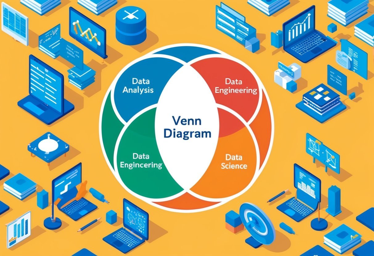
A Venn diagram with three overlapping circles representing data analysis, data engineering, and data science skills

Statistics and mathematics play a crucial role in data analysis and data science. From building predictive models to conducting statistical analysis, these disciplines provide the tools needed to transform raw data into meaningful insights.

Importance of Statistics in Data Analysis

Statistics is pivotal for analyzing and understanding data. It allows analysts to summarize large datasets, identify trends, and make informed decisions.

Statistical analysis involves techniques like descriptive statistics, which describe basic features of data, and inferential statistics, which help in making predictions.

By leveraging statistics, data professionals can create predictive models that forecast future trends based on current data.

These models use probability theory to estimate the likelihood of various outcomes. Understanding statistical modeling enables analysts to identify relationships and trends, which is critical in fields like finance, healthcare, and technology.

Mathematical Concepts Underpinning Data Work

Mathematics provides a foundation for many data-related processes. Concepts such as linear algebra, calculus, and probability are essential in data science.

Linear algebra is used for working with data structures like matrices, which help in organizing and manipulating datasets efficiently. Calculus aids in optimizing algorithms and understanding changes in variables.

Incorporating mathematical concepts enhances the ability to build complex models and perform detailed data analysis.

For example, probabilistic methods help in dealing with uncertainty and variability in data. By grasping these mathematical foundations, professionals can develop robust models and perform sophisticated analyses, which are essential for extracting actionable insights from data.

Creating and Maintaining Robust Data Infrastructures

A network of interconnected gears, wires, and circuit boards representing the intersection of data analysis, data engineering, and data science

Building strong data infrastructures is key for supporting data-driven decision-making. It involves designing systems that can scale and efficiently handle data. Managing data pipelines and warehousing ensures data moves reliably across platforms.

Designing Scalable Data Architecture

Designing scalable data architecture is crucial for handling large volumes of information. It often includes technologies like Hadoop and Spark, which can process big data efficiently.

These systems are designed to grow with demand, ensuring that as more data flows in, the architecture can handle it seamlessly.

Cloud platforms such as AWS, Azure, and GCP provide on-demand resources that are both flexible and cost-effective.

Using data lakes and smaller distributed systems can further improve scalability by organizing data without the limitations of traditional data warehouses. Implementing Apache Spark for distributed data processing ensures quick analysis and insights.

Managing Data Pipelines and Warehousing

Data pipelines are automated processes that move data from one system to another while performing transformations. Tools like Apache Airflow are popular for orchestrating complex workflows.

These pipelines need to be reliable to ensure that data arrives correctly formatted at its destination.

ETL (Extract, Transform, Load) processes are vital for data warehousing, as they prepare data for analysis. Data warehousing systems store and manage large datasets, providing a central location for analysis.

Technologies such as AWS Redshift or Google BigQuery enable quick querying of stored data. Maintaining a robust pipeline architecture helps companies keep data consistent and accessible for real-time analytics.

Advanced Analytical Techniques and Algorithms

A web of interconnected gears, circuit boards, and data visualizations overlapping and merging together

Advanced analytical techniques integrate predictive modeling and machine learning to enhance data analysis. These approaches leverage tools like scikit-learn and TensorFlow for developing robust models and algorithms. Utilizing these methods empowers professionals to manage big data and implement effective data mining strategies.

Developing Predictive Models and Algorithms

Predictive modeling involves creating a mathematical framework that forecasts outcomes using existing data. It requires the selection of appropriate algorithms, which can range from simple linear regression to complex neural networks.

These models analyze historical data to predict future events, aiding decision-makers in strategic planning.

Tools like scikit-learn simplify the process by providing a library of algorithms suitable for various data structures. Data scientists often select models based on factors like accuracy, speed, and scalability.

Big data processing helps improve model accuracy by providing a wider range of information. An effective approach combines model training with real-world testing, ensuring reliability and practicality.

Machine Learning and Its Applications

Machine learning (ML) utilizes algorithms to enable systems to learn and improve from experience. Its primary focus is to develop self-learning models that enhance decision-making without explicit programming.

Artificial intelligence drives innovation in machine learning by simulating human-like learning processes.

Applications of ML include classification, clustering, and regression tasks in areas like finance, healthcare, and marketing.

Technologies like TensorFlow facilitate the creation of complex neural networks, enabling high-level computations and simulations. Data engineers harness ML to automate data processing, improving efficiency in handling vast datasets.

Proper algorithm selection is key, with specialists often tailoring algorithms to suit specific requirements or constraints.

Insightful Data Visualization and Reporting

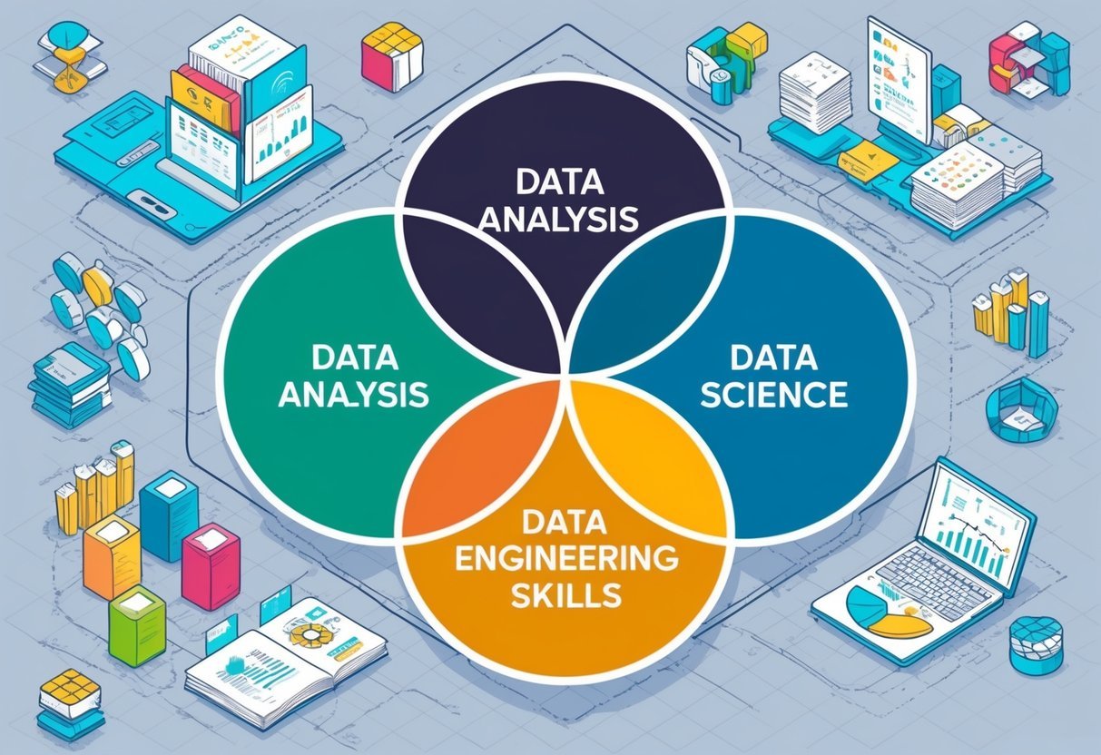
A Venn diagram with three overlapping circles representing data analysis, data engineering, and data science skills

Data visualization is essential for turning raw data into meaningful insights. Effective reporting can shape business decisions, creating a clear narrative from complex data sets. With the right tools and techniques, anyone can develop a strong understanding of data trends and patterns.

Crafting Data Stories with Visuals

Visual storytelling in data isn’t just about making charts; it’s about framing data in a way that appeals to the audience’s logic and emotions. By using elements like color, scale, and patterns, visuals can highlight trends and outliers.

Tools like Tableau and Power BI allow users to create interactive dashboards that present data narratives effectively. This approach helps the audience quickly grasp insights without slogging through spreadsheets and numbers.

Incorporating visuals into reports enhances comprehension and retention. Presenting data through graphs, heat maps, or infographics can simplify complex datasets.

These visuals guide the reader to understand the story the data is telling, whether it’s tracking sales growth or understanding user engagement patterns. A well-crafted visual can transform dry statistics into a compelling narrative that drives business strategy.

Tools for Communicating Data Insights

Choosing the right tool for data visualization is crucial. Popular options include Tableau, which offers robust features for creating interactive dashboards, and Power BI, known for its compatibility with Microsoft products.

Both allow users to turn data into dynamic stories. They support a range of data sources, making them versatile options for diverse business intelligence needs.

For those familiar with coding, Jupyter Notebook is an excellent choice. It integrates data analysis, visualization, and documentation in one place. The flexibility in such tools allows users to compile and present data insights in a cohesive manner.

Selecting the most fitting tool depends on the specific needs, complexity of data, and the user’s expertise in handling these platforms.

Data Quality and Governance for Informed Decisions

A bustling office with three interconnected circles representing data analysis, data engineering, and data science. A prominent sign reads "Data Quality and Governance for Informed Decisions."

Data quality and governance are essential for organizations aiming to make accurate data-driven decisions. High-quality data and effective governance practices ensure that business decisions are backed by reliable and actionable insights.

Ensuring High-Quality Data Output

High-quality data is accurate, complete, and reliable. These characteristics are vital in making data-driven decisions.

Poor data quality can lead to incorrect or incomplete insights, which negatively impacts business strategies.

Organizations must focus on maintaining data quality to ensure that the insights derived from it are trustworthy. This involves regular checks and validation processes.

Using advanced tools and methodologies, like data cleaning and transformation, organizations can improve data quality. This enhances their ability to extract actionable insights from datasets.

Accurate data collection, entry, and storage practices are equally important.

Data Governance and Ethical Considerations

Data governance is a framework that ensures data is used appropriately and ethically. It involves setting policies and practices that guide the responsible use of data.

Effective governance establishes clear roles and responsibilities for data management.

Organizations must focus on data security, privacy, and compliance with laws to maintain trust with stakeholders. Ethical considerations in data usage also include ensuring transparency and fairness in data handling.

Implementing a robust data governance strategy supports informed business decisions and strengthens data-driven processes. Moreover, maintaining high data governance standards helps organizations avoid legal and ethical pitfalls.

To learn more about how data governance can improve data quality, visit the Data Governance Improves Data Quality page.

Building and Leading Effective Data Teams

A group of people with diverse backgrounds collaborate around a table, exchanging ideas and working together on data-related projects

Establishing effective data teams requires a balance of technical skills and collaboration.

Focus on encouraging domain expertise and clear communication among various roles to ensure successful teamwork.

Cultivating Domain Expertise Among Teams

Domain expertise is essential in data teams, as it deepens the team’s ability to interpret data insights accurately. Team members must develop an understanding of industry-specific concepts and challenges.

This knowledge allows data scientists and analysts to tailor their approaches to solve real-world problems better.

Training programs and workshops can be beneficial in fostering domain-specific skills. Encouraging team members to engage with industry publications and attend relevant conferences further enhances their knowledge.

These activities should be complemented by mentoring sessions, where experienced team members share insights with newer ones, fostering a culture of continuous learning and expertise growth.

Roles and Collaboration within Data Organizations

A successful data organization is one where roles are clearly defined but flexible enough to promote collaboration.

Key roles include data engineers, who manage data infrastructure, and data analysts, who interpret data using visualization tools. Data scientists often focus on creating predictive models.

Effective collaboration is fostered by encouraging open communication and regular cross-functional meetings. Tools like collaborative platforms and dashboards help keep workflow and progress transparent, allowing team members to identify and address potential issues.

Emphasizing teamwork over individual effort and recognizing collaborative achievements can significantly enhance the team’s cohesion and productivity.

Navigating Career Paths in Data Professions

A person analyzing data, building systems, and conducting experiments

Entering the realm of data professions requires a clear understanding of the right educational background and a keen insight into market trends. These insights help shape successful careers in data-related fields, from data analysis to data science.

Evaluating Data-Related Educational Backgrounds

Choosing the correct educational path is crucial for anyone aspiring to enter data professions. A bachelor’s degree in fields such as computer science, statistics, or mathematics can provide a strong foundation.

However, degrees aren’t the only path. Bootcamps and short courses offer focused training in practical skills relevant to data roles.

For those focusing on data analysis or engineering, knowledge in programming languages like Python and SQL is invaluable. Meanwhile, data scientists might benefit more from proficiency in machine learning frameworks.

Each career path has specific skills and qualifications, which aspiring professionals must consider to enhance their career opportunities.

Understanding the Market and Salary Trends

The demand for data professionals continues to grow, influencing market trends and salary expectations.

Professionals equipped with the right skills find themselves in a favorable career outlook.

Salaries can vary significantly based on role and experience level. For instance, entry-level data analysts might see different compensation compared to data scientists or engineers.

Reviewing resources like the Data Science Roadmap helps in estimating potential earnings.

Furthermore, regions play a role in salary variations. Typically, urban centers offer higher compensation, reflecting the demand and cost of living in these areas. Understanding these trends assists individuals in making informed career decisions.

Evolution and Future Trends in Data Ecosystems

Data ecosystems are rapidly evolving with advanced technologies and strategies. The focus is shifting towards more integrated and efficient systems that leverage emerging technologies in big data platforms and data-driven AI strategies.

Emerging Technologies in Big Data Platforms

Big data platforms are transforming with new technologies to handle increasingly complex data. Systems like Hadoop and Storm are being updated for better performance.

Advanced analytics tools play a crucial role in extracting valuable insights and enabling more accurate predictive analytics.

This involves processing vast amounts of information efficiently and requires innovative solutions in storage and retrieval.

As part of this evolution, the need for improved software engineering practices is evident. Developers are focusing on real-time data processing, scalability, and flexibility to support diverse applications across industries.

The Move Towards Data-Driven AI Strategies

AI strategies increasingly depend on data ecosystems that can effectively support machine learning models and decision-making processes.

A shift towards data-driven approaches enables organizations to realize more precise predictions and automated solutions.

This trend emphasizes the integration of robust data management practices and innovative big data platforms.

By linking AI with vast datasets, businesses aim to gain a competitive edge through insightful, actionable intelligence.

Investments in AI-driven platforms highlight the importance of scalable data architectures that facilitate continuous learning and adaptation. Companies are enhancing their capabilities to support advanced use cases, focusing on infrastructure that can grow with evolving AI needs.

Frequently Asked Questions

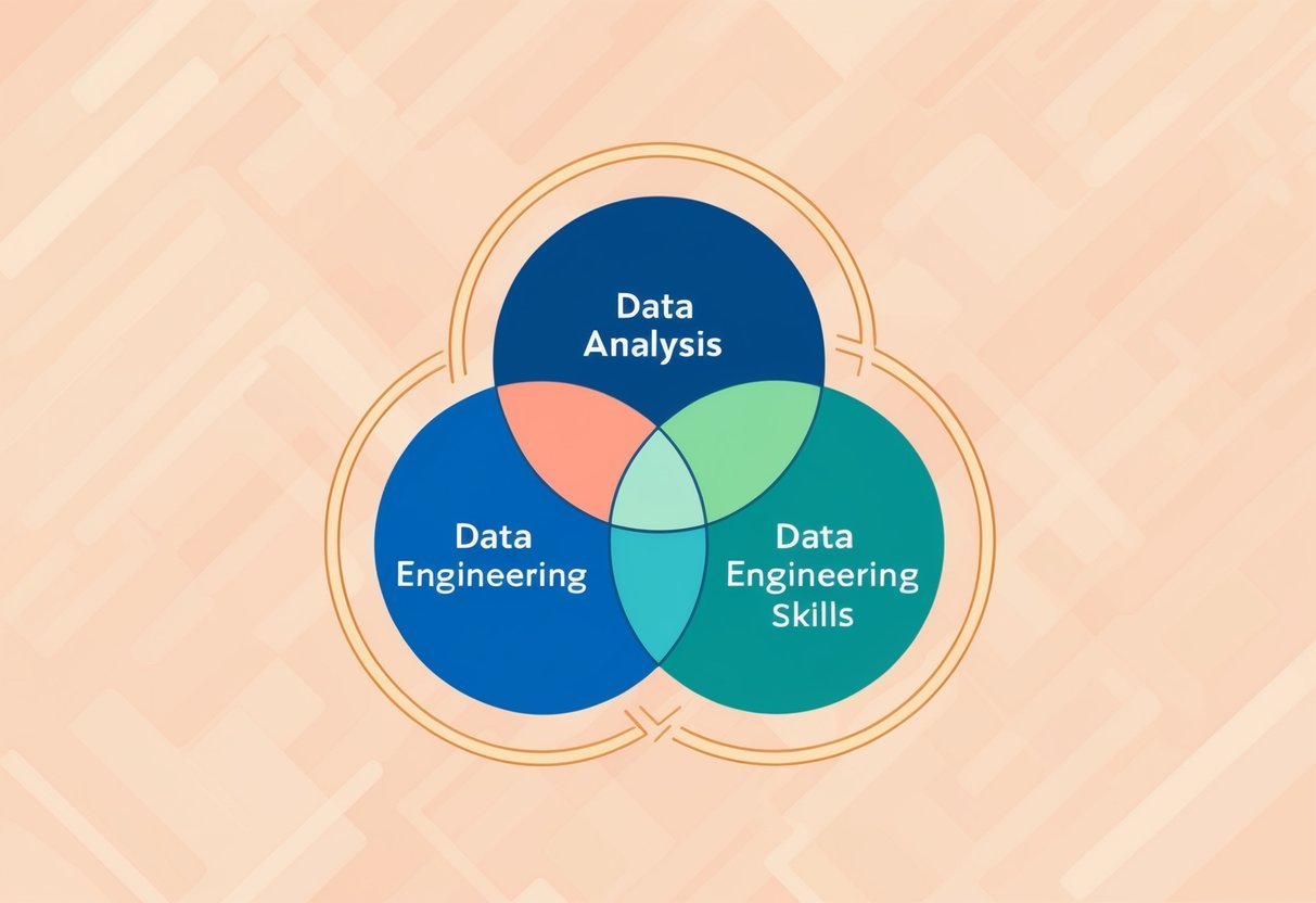
A Venn diagram with three overlapping circles representing data analysis, data engineering, and data science skills

When exploring careers in data-related fields, it is important to understand the distinct roles and required skills. Data analysis, data engineering, and data science each have specific demands and responsibilities. Knowing these differences can guide career choices and skill development.

What distinct technical skill sets are required for a career in data analysis compared to data science?

Data analysts often focus on statistical analysis and data visualization. They need proficiency in tools like Excel and Tableau.

Data scientists, in contrast, typically need a deeper understanding of programming, machine learning, and algorithm development. Python and R are common programming languages for data scientists, as these languages support sophisticated data manipulation and modeling.

How does the role of a data engineer differ from a data analyst in terms of daily responsibilities?

Data engineers design, build, and maintain databases. They ensure that data pipelines are efficient and that data is available for analysis.

Their day-to-day tasks include working with big data tools and programming. Data analysts, on the other hand, spend more time exploring data and identifying patterns to inform business decisions.

What are the fundamental programming languages and tools that both data scientists and data analysts must be proficient in?

Both data scientists and data analysts commonly use programming languages like Python and R. These languages help with data manipulation and analysis.

Tools such as SQL are also essential for handling databases. Familiarity with data visualization tools like Tableau is critical for both roles to present data visually.

Which methodologies in data management are essential for data engineers?

Data engineers must be knowledgeable about data warehousing, ETL (Extract, Transform, Load) processes, and data architecture.

Understanding how to manage and organize data efficiently helps in building robust and scalable data systems. This knowledge ensures that data is clean, reliable, and ready for analysis by other data professionals.

Categories
Uncategorized

Learning about SQL Generating Data Series with Recursive CTEs: A Clear Guide

Understanding Common Table Expressions (CTEs)

Common Table Expressions (CTEs) are a powerful feature in SQL used to simplify complex queries and enhance code readability.

CTEs are defined with the WITH clause and can be referred to in subsequent SQL statements, acting as a temporary named result set.

Defining CTEs and Their Uses

CTEs, or Common Table Expressions, provide a way to structure SQL queries more clearly. They are defined using the WITH clause and can be used in a variety of SQL operations like SELECT, INSERT, UPDATE, or DELETE.

CTEs help in breaking down complex queries into simpler parts.

A key benefit of CTEs is improving the readability and maintainability of code. They allow users to create temporary named result sets, which makes code more understandable.

This is particularly useful when dealing with recursive queries or when needing to reference the same complex logic multiple times in a single SQL statement.

CTEs also assist in handling hierarchical data and recursive data structures. This makes them versatile for tasks requiring data aggregation or when complex joins are necessary.

By using CTEs, developers can implement cleaner and more efficient solutions to intricate data problems.

Anatomy of a CTE Query

A typical CTE query starts with the WITH keyword, followed by the CTE name and a query that generates the temporary result set. The basic syntax is:

WITH cte_name AS (
    SELECT column1, column2
    FROM table_name
    WHERE condition
)
SELECT *
FROM cte_name;

In the example above, cte_name is the temporary named result set. The CTE can then be referenced in the SELECT statement that follows. This structure facilitates the separation of complex logic into manageable parts.

CTE queries often simplify the querying process by removing the need for nested subqueries.

Multiple CTEs can be chained together, each defined in sequence, to build upon one another within a single SQL statement. This flexibility is crucial for developing scalable and efficient database queries.

Fundamentals of Recursive CTEs

Recursive Common Table Expressions (CTEs) are crucial in SQL for dealing with hierarchical or tree-structured data. They work by repeatedly using results from one pass of a query as input for the next. This helps in simplifying complex queries and reduces the need for procedural code.

Recursive CTE Components

A recursive CTE consists of two main parts: the anchor member and the recursive member.

The anchor member provides the initial dataset. It is often a base query that sets the starting point for the recursion. In SQL syntax, it’s the part that gets executed first, laying the foundation.

The recursive member is built on the results obtained from the anchor state. It usually references itself to keep iterating over the data. This member runs until a termination condition is met, avoiding infinite loops.

The recursive member helps dive deeper into the dataset, allowing it to expand until all specified conditions are satisfied.

The Role of Recursion in SQL

Recursion in SQL through CTEs allows for the processing of hierarchical data effectively. For example, when handling organizational charts or file directory structures, recursion facilitates exploring each level of hierarchy.

This type of query references itself until all necessary data points are retrieved.

The use of recursion enables SQL to execute operations that require a loop or repeated execution, which can be represented as a simple SQL statement. It streamlines data manipulation and enhances the readability of complex queries.

Recursion is powerful when evaluating relationships within data sets, reducing the complexity of nested queries.

Configuring Recursive CTEs

Recursive CTEs in SQL are used to work with hierarchical and iterative data structures. Setting up involves defining an anchor member and then the recursive member, ensuring a correct flow and exit to prevent infinite loops.

Setting Up an Anchor Member

The anchor member forms the base query in a recursive CTE. This part of the query defines the starting point of the data set and is executed only once.

It’s crucial because it determines the initial result set, which will subsequently feed into recursive iterations.

A simple example involves listing dates from a start date. The anchor member might select this start date as the initial entry.

For instance, to list days from a particular Monday, the query would select this date, ensuring it matches the format required for further operations.

This sets up the basic structure for subsequent calculations, preparing the ground for recursive processing with clarity and precision.

Formulating the Recursive Member

The recursive member is central to expanding the initial result set obtained by the anchor member. It involves additional queries that are applied repeatedly, controlled by a union all operation that combines these results seamlessly with the anchor data. This step is where recursion actually happens.

Termination conditions are vital in this part to prevent infinite loops.

For instance, when listing days of the week, the condition might stop the recursion once Sunday is reached. This is achieved by setting parameters such as n < 6 when using date functions in SQL.

Proper formulation and planning of the recursive member ensure the desired data set evolves precisely with minimal computation overhead.

Constructing Hierarchical Structures

Hierarchical structures are common in databases, representing data like organizational charts and family trees. Using Recursive Common Table Expressions (CTEs) in SQL, these structures are efficiently modeled, allowing for nuanced data retrieval and manipulation.

Representing Hierarchies with CTEs

Recursive CTEs are essential tools when dealing with hierarchical data. They enable the breakdown of complex relationships into manageable parts.

For example, in an organizational chart, a manager and their subordinates form a hierarchy.

The use of recursive CTEs can map these relationships by connecting manager_id to staff entries. This process involves specifying a base query and building upon it with recursive logic.

A critical step is establishing the recursion with a UNION ALL clause, which helps connect each staff member to their respective manager.

In constructing these queries, one can create clear pathways from one hierarchy level to the next.

Hierarchical and Recursive Queries in SQL Server provide a deeper insight into this process, offering practical examples for better representation of organizational structures.

Navigating Complex Relationships

Navigating complex relationships is crucial for interpreting data structures like family trees and corporate hierarchies. Recursive CTEs facilitate efficient data traversal by repeatedly applying a set of rules to extract information at different levels.

When dealing with an organization, each manager and their subordinates can be connected recursively. The recursive query technique helps in understanding the reporting structure and paths in intricate setups.

For instance, finding all employees under a certain manager involves starting from a node and traversing through connected nodes recursively.

Leveraging tools and guides, such as this one on writing recursive CTEs, enhances the ability to manage and navigate data intricacies effectively.

These methods provide clear direction for accessing and interpreting all levels of a hierarchy, making SQL a powerful tool for managing complex data landscapes.

Advanced Use Cases for Recursive CTEs

Recursive CTEs are powerful tools in SQL, especially useful for tasks involving hierarchical and network data. They can simplify complex queries and make data analysis more efficient.

Analyzing Bill of Materials

In manufacturing, the Bill of Materials (BOM) is crucial for understanding product composition. It details all components and subcomponents needed to manufacture a product.

Recursive CTEs are ideal for querying this structured data. They allow users to explore multi-level relationships, such as finding all parts required for a product assembly.

For instance, a CTE can repeatedly query each level of product hierarchy to compile a complete list of components. This approach ensures a comprehensive view of the materials, helping to optimize inventory and production processes.

Modeling Social Networks

In social networks, understanding connections between individuals is essential. Recursive CTEs help to analyze and display these relationships efficiently.

Using these CTEs, one can trace social connections to identify potential influence networks or clusters of close-knit users.

For example, a query may identify all direct and indirect friendships, providing insights into the spread of information or trends.

By leveraging Recursive CTEs, analyzing social structures becomes streamlined, facilitating better decision-making for network growth and engagement strategies.

This ability to manage intricate relational data sets makes Recursive CTEs indispensable in social network analysis.

Handling SQL Server-Specific CTE Features

A computer screen displaying SQL code with recursive CTEs generating data series

Using SQL Server, one can take advantage of specific features when working with CTEs. Understanding how to implement recursive queries and the certain optimizations and limitations are crucial to maximizing their potential.

Exploring SQL Server Recursive CTEs

In SQL Server, recursive CTEs are a powerful way to generate sequences of data or explore hierarchical data. The recursive process begins with an anchor member, which establishes the starting point of the recursion.

After this, the recursive member repeatedly executes until no more rows can be returned.

A typical setup involves defining the CTE using the WITH keyword, and specifying both the anchor and recursive parts. For example, a basic CTE to generate a series might start with WITH CTE_Name AS (SELECT...).

Recursive queries handle situations like managing organizational hierarchies or finding paths in graphs, reducing the need for complex loops or cursors.

Recursive CTEs can depth-limit during execution to prevent endless loops, ensuring efficient processing. They are handy in scenarios where data relationships mimic a tree structure, such as company hierarchies.

To see more examples of working with recursive CTEs, including an explanation of SQL Server Recursive CTE, refer to practical articles.

Optimizations and Limitations on SQL Server

When working with CTEs, SQL Server provides optimizations to improve performance. One such feature is query execution plans, which SQL Server uses to find the most efficient way to execute statements.

Understanding these plans helps identify bottlenecks and optimize recursive CTE performance.

However, SQL Server’s CTEs have limitations. The maximum recursion level is set to 100 by default, which means that queries exceeding this limit will fail unless specifically adjusted using OPTION (MAXRECURSION x).

Also, while useful, recursive CTEs can be less efficient than other methods for large datasets or deep recursions due to memory usage.

Recognizing these constraints helps developers make informed decisions when using recursive CTEs within SQL Server. For more techniques and detail on how SQL Server handles recursive queries, see the SQL Server handle recursive CTE’s.

Preventing Infinite Loops in Recursive CTEs

A computer screen displaying a SQL script with a recursive common table expression generating a data series, with a focus on preventing infinite loops

Recursive CTEs are powerful tools in SQL that allow users to perform complex queries. However, they can sometimes result in infinite loops if not carefully managed.

Ensuring that these queries execute correctly is crucial.

One way to prevent infinite loops is to implement a termination condition. This involves setting a limit that stops the recursion when a certain condition is met.

For example, using a WHERE clause helps end the loop when a specific value is reached. A condition like WHERE level <= 4 allows for safe execution.

Different SQL systems may also allow for configuring a maximum recursion depth. This setting is often adjustable and starts at a default, commonly 100, to cap how many times the recursion can occur.

This feature acts as a built-in safeguard to halt potential infinite loops.

Additionally, incorporating stops in the logic of the recursive CTE can aid in preventing loops. This means avoiding scenarios where the loop might travel back to previous values, forming a cycle.

Moreover, database engines often have mechanisms to detect and break loops if they happen, but it’s best to handle such risks through careful query design.

Lastly, using unique identifiers within the recursive CTE structure can help maintain a clear path and avoid cycles.

Applying these practices ensures safer and more effective use of recursive CTEs, helping users utilize their full potential without encountering infinite loop issues.

Working with Temporary Tables and CTEs

A computer screen displaying SQL code for temporary tables and recursive CTEs

Understanding the roles and differences between temporary tables and Common Table Expressions (CTEs) is key when working with SQL. Each serves unique purposes and can optimize specific tasks within databases.

Differences Between Temporary Tables and CTEs

A temporary table is a physical table. It exists for the duration of a session or until it is explicitly dropped. They are useful when dealing with large datasets because they can store intermediate results. This helps reduce the complexity of SQL queries.

Temporary tables can handle indexed operations, allowing for faster access to data.

Common Table Expressions (CTEs), on the other hand, create a temporary result set that only exists within a query’s scope. They are defined with WITH and are useful for readability and modularizing complex queries.

CTEs do not allow indexing, which may affect performance with large datasets.

Choosing Between CTEs and Temporary Tables

When deciding between a temporary table and a CTE, consider the size of the dataset and the complexity of the query.

For small to medium datasets, CTEs can simplify the query process. They are effective for queries where the data does not need to persist beyond the query execution.

Recursive operations, such as hierarchical data traversals, are well-suited for recursive CTEs.

Temporary tables are ideal for large datasets or when multiple operations on the data are necessary. Since they support indexing, temporary tables may improve performance for certain operations.

Also, if multiple queries need to access the same temporary dataset, creating a temporary table might be more efficient.

Common Pitfalls and Best Practices

A computer screen displaying SQL code for generating data series with Recursive CTEs, surrounded by books on SQL best practices

Recursive CTEs are a powerful tool, yet they come with challenges. Understanding how to avoid common pitfalls and implement best practices helps improve performance and maintain complex queries effectively.

Avoiding Common Errors With Recursive CTEs

One common error with recursive CTEs is infinite recursion, which occurs when the termination condition is not specified correctly. It is essential to add a clear exit criterion to avoid running indefinitely.

When constructing a recursive query, ensuring that every iteration reduces the result set is crucial. This guarantees that the CTE eventually finishes execution.

Another mistake is excessive memory usage. Recursive CTEs can consume large amounts of resources if not designed carefully.

Limiting the dataset processed in each iteration helps manage memory more efficiently. Using indexes on columns involved in joins or filters can also enhance query performance.

Debugging recursive CTEs can be challenging. It helps to test each part of the query separately.

Beginning with static data before introducing recursion can make troubleshooting easier. By doing this, the user can identify issues early on and adjust incrementally.

Implementing Best Practices for Performance

To optimize recursive CTEs, using clear naming conventions is advised. This helps differentiate base and recursive components, which aids readability and maintenance.

Keeping the query simple and focused on a specific task avoids unnecessary complexity.

Monitoring query performance using execution plans can highlight areas that cause slowdowns. If a CTE grows too complex, breaking it into smaller, logical parts may help. This allows easier optimization and understanding of each segment’s role in the query.

Additionally, when necessary, use non-recursive CTEs for parts of the query that do not require recursion. This can minimize overhead and speed up execution.

Setting an appropriate MAXRECURSION limit can prevent endless loops and unintended server strain.

Developing SQL Skills with Recursive CTEs

A computer screen displaying SQL code with recursive CTEs generating a data series

Recursive CTEs are a valuable tool for developing SQL skills. They allow users to efficiently handle hierarchical data, making them essential for complex queries. This method refers to itself within a query, enabling repeated execution until the full data set is generated.

Working with recursive CTEs enhances a user’s ability to write sophisticated SQL queries. These queries can solve real-world problems, such as navigating organizational charts or managing multi-level marketing databases.

Consider this simplified example:

WITH RECURSIVE Numbers AS (
    SELECT 1 AS n
    UNION ALL
    SELECT n + 1 FROM Numbers WHERE n < 5
)
SELECT * FROM Numbers;

This query generates a series of numbers from 1 to 5. By practicing with such queries, users improve their understanding of recursive logic in SQL.

Key Skills Enhanced:

  • Hierarchical Data Manipulation: Recursive CTEs allow users to work with data structured in a hierarchy, such as employee-manager relationships.

  • Problem Solving: Crafting queries for complex scenarios develops critical thinking and SQL problem-solving abilities.

  • Efficiency: Recursive queries often replace less efficient methods, streamlining processes and improving performance.

Understanding recursive CTEs requires practice and thoughtful experimentation. Resources like the guide on writing a recursive CTE in SQL Server and examples from SQL Server Tutorial are helpful. As they progress, users will find themselves better equipped to tackle increasingly challenging SQL tasks.

Application in Data Science

A computer screen displaying a SQL code editor with a series of recursive common table expressions generating data for data science learning

In data science, understanding data hierarchies is essential. Recursive CTEs can efficiently query hierarchical data. For example, they are used to explore organizational structures by breaking down data into related levels. This approach simplifies complex data patterns, making analysis more manageable.

Recursive queries also help in generating data series. These are useful for creating test datasets. By establishing a starting condition and a recursive step, data scientists can create these series directly in SQL. This approach saves time and effort compared to manual data generation.

Recursive CTEs can also assist with pathfinding problems. These queries help trace paths in networks, like finding shortest paths in a graph. This is particularly beneficial when analyzing network traffic or connections between entities.

Furthermore, data scientists often need to deal with unstructured data. Recursive queries enable them to structure this data into meaningful insights.

By breaking complex datasets into simpler components, recursive CTEs add clarity and depth to data analysis, ultimately enhancing the understanding of intricate data relationships.

Analyzing data science workflows often requires advanced SQL techniques like recursive CTEs, which streamline processes and increase efficiency. Mastery of these techniques empowers data scientists to tackle challenging tasks involving complex data hierarchies and relationships.

Generating Data Series with Recursive CTEs

A computer screen displaying a series of code lines, with a database diagram in the background

Recursive Common Table Expressions (CTEs) are a powerful tool in SQL that allow users to generate data series efficiently. They are especially useful for creating sequences of dates and numbers without needing extensive code or external scripts.

Creating Sequences of Dates

Creating a sequence of dates using recursive CTEs is a practical solution for generating timelines or schedules. A recursive CTE can start with an initial date and repeatedly add days until the desired range is complete.

By utilizing a recursive query, users can generate sequences that include only weekdays. This is accomplished by filtering out weekends, typically using a function or a condition in the WHERE clause.

Here is an example structure:

WITH DateSeries AS (
    SELECT CAST('2024-01-01' AS DATE) AS Date
    UNION ALL
    SELECT DATEADD(DAY, 1, Date)
    FROM DateSeries
    WHERE DATEPART(WEEKDAY, DATEADD(DAY, 1, Date)) BETWEEN 2 AND 6
    AND Date < CAST('2024-01-31' AS DATE)
)
SELECT Date FROM DateSeries;

This query generates a date series from January 1st to January 31st, only including weekdays.

Generating Numeric Series

For numerical data, recursive CTEs efficiently create ranges or sequences. They are ideal for tasks such as generating numbers for analytical purposes or filling gaps in data.

To create a numeric series, start with a base number and increment it in a loop until reaching the target value. Recursive CTEs can be more efficient than other methods like loops due to their set-based approach.

Below is an example:

WITH Numbers AS (
    SELECT 1 AS Number
    UNION ALL
    SELECT Number + 1
    FROM Numbers
    WHERE Number < 100
)
SELECT Number FROM Numbers;

This SQL code quickly generates numbers from 1 to 100, making it practical for various applications where numeric series are required.

Frequently Asked Questions

A computer screen displaying SQL code for generating data series with Recursive CTEs, surrounded by FAQ materials

Recursive CTEs in SQL offer a dynamic way to generate series such as date sequences, perform hierarchical queries, and optimize performance in databases. Understanding the differences between recursive and standard CTEs is crucial for effective use.

How can I use recursive CTEs to generate a date series in SQL?

Recursive CTEs can be used to create a sequence of dates by iteratively computing the next date in a series. This is particularly useful for time-based analyses and reporting.

By starting with an initial date and iteratively adding intervals, one can efficiently generate a complete date range.

What are some real-world examples of recursive CTEs in SQL?

Recursive CTEs are commonly used in scenarios like hierarchies in organizational charts or generating sequences for calendar dates. Another example includes computing aggregate data over hierarchical structures, such as calculating the total sales of each department in a company.

Can you illustrate a recursive CTE implementation for hierarchical queries in SQL?

Hierarchical queries often involve retrieving data where each record relates to others in a parent-child manner. Using a recursive CTE, SQL can repeatedly traverse the hierarchy, such as finding all employees under a certain manager by starting with top-level employees and recursively fetching subordinates.

What are the main parts of a recursive common table expression in SQL?

A recursive CTE consists of two main parts: the anchor member and the recursive member. The anchor member defines the initial query. The recursive member references the CTE itself, allowing it to repeat and build on results until the complete dataset is processed.

How to optimize performance when working with recursive CTEs in SQL Server?

Optimizing recursive CTEs involves strategies like limiting recursion to avoid excessive computation and using appropriate indexes to speed up query execution.

Careful use of where clauses can ensure that only necessary data is processed, improving efficiency.

What is the difference between a recursive CTE and a standard CTE in SQL?

The primary difference is that a recursive CTE references itself within its definition, allowing it to iterate over its results to generate additional data.

A standard CTE does not have this self-referential capability and typically serves as a temporary table to simplify complex queries.

Categories
Uncategorized

Learning Power BI – Data Visualization: Mastering Reports and Dashboards

Getting Started with Power BI

Power BI is a powerful tool from Microsoft designed for users to create reports and dashboards that enhance business intelligence and data visualization. Mastering it allows creating interactive and insightful visuals, improving user experience.

Overview of Power BI

Power BI is a suite of business analytics tools that assist in transforming raw data into meaningful insights.

It comprises several components, including Power BI Desktop, Power BI Service, and Power BI Mobile. Each component has specific features designed to cater to different needs, such as creating content on the desktop app or sharing and viewing reports online using the service.

Users can import data from various sources like Excel, databases, or cloud services. Using these sources, they can build interactive visuals and share them with their teams.

This integration supports diverse data visualization needs, making it easier for businesses to analyze and monitor essential metrics.

Power BI enhances user experience through its intuitive design that doesn’t require extensive technical knowledge. Users can efficiently create dashboards that display data in an understandable format, benefiting strategic decision-making processes in any organization.

Explore more in guides like Microsoft Power BI Dashboards Step by Step.

Building Blocks of Power BI

Power BI is a powerful tool for creating reports and dashboards. It relies on two main components to deliver its features: Power BI Desktop and the Power BI Service. Each plays a crucial role in how businesses utilize data for actionable insights.

Understanding Power BI Desktop

Power BI Desktop is the starting point for creating compelling data visuals. Users first import data from various sources into the software which supports numerous file formats.

Cleaning and transforming data is crucial, and Power BI Desktop offers tools for refining data sets.

Once data preparation is complete, users can build interactive reports. The drag-and-drop interface makes creating visuals straightforward, even for beginners.

Visuals can include charts, graphs, and maps, and users have options to customize these elements to meet their needs. Advanced users may employ DAX (Data Analysis Expressions) for more complex data manipulations.

The desktop application not only aids in designing reports but also allows users to test and visualize data transformations.

Exploring the Power BI Service

The Power BI Service extends the capabilities of the desktop application by allowing for sharing and collaboration.

After reports are ready in Power BI Desktop, they are published to the cloud-based Power BI Service for wider distribution. Here, teams can access and interact with shared content on various devices.

This service is crucial for businesses needing up-to-date data insights. Users can harness real-time dashboards, set alerts, and even embed Power BI reports into existing business software platforms.

The service’s collaborative features ensure that insights are not just created but also shared across teams efficiently. Data security and governance are built-in features, keeping sensitive information protected while still being widely accessible to authorized users.

Data Analysis Fundamentals

A computer screen displaying a Power BI dashboard with colorful charts and graphs, surrounded by a cluttered desk with notebooks and pens

In Power BI, understanding data analysis fundamentals is key to creating effective reports and dashboards. This involves importing and transforming data along with using DAX formulas and functions to derive insights.

Importing Data

Importing data in Power BI is the first step in building data models. Users can bring in data from various sources such as Excel, SQL Server, and online services. Power BI supports diverse data formats, ensuring flexibility in how researchers handle their data.

A successful import includes choosing the right data connectors. Users must also consider the structure and quality of incoming data. Sometimes, initial data cleaning might be necessary to ensure accuracy.

This stage sets the foundation for all analyses and determines how effectively insights can be drawn from the data set.

Transforming Data

Once data is imported, transforming it is essential for meaningful analysis. Power BI’s Power Query Editor is a robust tool used for data shaping.

This process involves cleaning and preparing data, like removing duplicates, combining tables, and changing data types to match analysis needs.

Transformation ensures data consistency and relevancy. Users can also perform calculations or create new data columns to aid in analysis.

Well-prepared data supports more accurate dashboards and helps in uncovering trends and patterns. Proper transformation makes subsequent data modeling and visualization straightforward and efficient.

DAX Formulas and Functions

DAX (Data Analysis Expressions) is a rich library of formulas and functions in Power BI essential for enhancing data analysis.

DAX is used to create calculated columns, measures, and custom tables, offering users flexibility in analyzing complex data sets.

Understanding DAX syntax and its diverse functions allows users to perform advanced calculations efficiently. Functions like SUM, AVERAGE, and FILTER are commonly used to manipulate data.

Mastery of DAX helps craft precise insights and supports dynamic, interactive reports and dashboards. It empowers users to perform both simple and complex data analysis with ease.

Crafting Power BI Reports

Developing effective Power BI reports requires understanding design principles, creating engaging visualizations, and knowing how to publish them. These steps ensure that reports are not only visually appealing but also informative and accessible to the intended audience.

Design Principles

When crafting Power BI reports, design principles play a crucial role. A well-designed report should be clean, with intuitive navigation and layout. It is important to maintain consistency in colors, fonts, and styles to create a professional look.

Organize data logically, and consider the audience’s needs and preferences. Use whitespace effectively to avoid clutter and guide the reader’s eye to important information.

Highlighting key metrics and using visual hierarchies can further enhance comprehension.

Aligning report elements and keeping interactive features user-friendly are also essential. This approach ensures that readers focus on the data presented without getting distracted.

Creating Visualizations

Creating effective visualizations is a vital part of crafting Power BI reports. Choose appropriate chart types that best represent the data, like bar or line charts for trends and pie charts for proportions.

Power BI provides a suite of visualization features that allow for rich, interactive experiences. Users can connect with various data sources, ensuring they can create reports tailored to specific insights.

Using filters and slicers can help users interact with the data dynamically.

It’s important to label axes and data points clearly, avoid misleading scales, and use color to distinguish information. Providing tooltips with additional data can also be beneficial for deeper insights without cluttering the main display.

Publishing Reports

The final step is publishing reports for access and further analysis. In Power BI, publishing allows reports to be shared across the organization or with specific individuals.

Consider the security and privacy settings while sharing these reports to ensure sensitive data remains protected.

The reports can be configured for online access through Power BI Service, where users can view updates in real-time.

Publishing should align with audience needs, ensuring accessibility on various devices like tablets and smartphones.

Dashboards in Detail

Understanding how to create, maintain, and utilize dashboards effectively is essential for leveraging data to drive decisions. This section explores the crucial aspects of designing interactive experiences and methods for sharing insights.

Concepts of Dashboards

A dashboard is a visual display of key data points and trends that help users understand large volumes of information at a glance. They are designed to showcase both summary and detailed data using elements like charts, graphs, and tables.

Dashboards should be focused and concise to ensure quick comprehension. The design should prioritize important metrics and use visual elements to highlight trends or potential issues. Consistency in layout and colors helps maintain clarity and aids users in navigating through different sections easily.

Key Features:

  • Visual representation of data
  • Real-time data updates
  • Customizable components

Effective dashboards provide users with the ability to make informed decisions based on data insights. They cater to different user needs, from executives seeking high-level overviews to analysts requiring in-depth data exploration.

Creating Interactive Dashboards

Creating interactive dashboards involves integrating features that allow users to engage with the data. Power BI offers tools to create dashboards where components such as filters and drill-through options enhance user interaction, making it a valuable platform for dynamic data exploration.

Interactive Elements:

  • Slicers and filters: Allow users to narrow down the data they view.
  • Drill-through functionality: Enables users to zoom into specific data points.
  • Responsive actions: Adjust based on user selections.

Embedding these interactive elements helps in providing a tailored experience to users, enabling them to derive specific insights without sifting through irrelevant data.

By allowing users to focus on pertinent information, these dashboards can improve decision-making at all levels.

Sharing and Exporting Dashboards

Sharing dashboards efficiently is essential for collaboration across teams and organizations. In Power BI, dashboards can be shared within an organization or exported for broader distribution. This ensures that stakeholders can access insights in formats that suit their requirements.

Methods to Share and Export:

  • Publishing to the web: Allows wider access and sharing links.
  • Exporting to PDFs or PowerPoint: Enables static report sharing.
  • Direct sharing in Power BI: Gives access to team members with permissions.

The ability to share and export dashboards ensures that valuable insights reach those who need them, fostering better communication and collaborative decisions.

Enhancing User Interaction

Enhancing user interaction in Power BI focuses on making dashboards more intuitive and engaging. Important features include using filters and slicers for personalized views and natural language queries for easier data exploration.

Filters and Slicers

Filters and slicers are essential tools for refining data views. They help users focus on specific data sets, enhancing the user experience by allowing personalized interactions with dashboards.

Filters can be applied at different levels, either to a whole report or just to individual visualizations.

Slicers provide a more visual way to filter information. Users can easily select options and see changes immediately, which is particularly beneficial in dynamic presentations. This immediate feedback helps users identify trends and insights more efficiently.

Utilizing filters and slicers enhances the usability of reports and dashboards. By giving users control over what they see, these tools make data interaction more intuitive and satisfying.

Natural Language Queries

Natural language queries in Power BI enable users to ask questions about their data using everyday language. This feature reduces the need for deep technical knowledge, making data exploration accessible to a broader audience.

Users can type simple questions and get visual answers, which can be faster than setting up traditional filters.

For example, typing “total sales last year” quickly displays relevant results without navigating complex menus. This helps in quickly gathering insights and understanding data trends.

Natural language capabilities are constantly improving, helping users get more accurate results even with complex queries. By supporting conversational interaction, this feature significantly enhances user experience, making it easier to gain insights from data.

Best Practices for Visualization

Creating meaningful data visualizations using Power BI involves selecting the right visual elements and weaving them into a coherent narrative. This helps businesses to derive insights efficiently from complex data sets.

Selecting Appropriate Visuals

Choosing the correct visuals for data representation is crucial. Bar charts are effective for comparing values across categories, while line graphs are perfect for illustrating trends over time.

For hierarchical data, consider using tree maps or sunburst charts. Scatter plots can display relationships between two variables.

Power BI offers a range of customizable charts and graphs. Users can tailor these to highlight the most significant insights.

Interactive features, such as drill-throughs or slicers, make it easier to explore data further. This helps users focus on what is most relevant to their analysis.

Data-Driven Storytelling

Data-driven storytelling combines data with narrative. This technique transforms raw data into a compelling story.

Power BI allows users to build dashboards that guide viewers through key insights. This structured approach helps convey complex information effectively.

Through consistent design elements like color schemes and layout, dashboards become more intuitive. This aids in ensuring that viewers grasp the intended message quickly.

Integrating textual elements to add context enhances understanding. Clear labels and titles help frame the insights drawn from the visualizations in Power BI.

Leveraging Power BI for Business

Power BI offers robust tools for businesses to analyze and communicate data effectively. By integrating business intelligence capabilities, companies can enhance decision-making processes and foster better communication with stakeholders.

Analyzing Business Metrics

Businesses can use Power BI to gain insights into complex data. With its powerful data analysis tools, it helps visualize key performance indicators and trends. This facilitates informed decision-making by highlighting areas that need attention or improvement.

Users can create interactive dashboards that provide real-time data. These dashboards offer the ability to drill down into specifics, offering a comprehensive view of business metrics.

Using features like data slicing, businesses can focus on particular aspects without losing sight of the overall picture.

The ability to combine data from various sources into a single view is another advantage. This integration ensures that businesses can evaluate metrics consistently and accurately. By leveraging these features, companies gain a significant advantage in competitive markets.

Communicating with Stakeholders

Power BI plays a crucial role in communication by translating technical data into understandable visuals. This ability is vital for stakeholders who need clarity to make strategic decisions.

Visual reports generated by Power BI help convey complex information in a clear and concise manner. Users can customize these reports to match the needs of different stakeholders, ensuring relevance and engagement.

Stakeholders benefit from the interactivity of the reports, allowing them to explore data points independently. This transparency fosters trust and collaboration.

By providing stakeholders with tailored insights, businesses ensure that everyone is aligned with the company’s goals and strategies.

Advancing Your Career with Power BI

A person using a computer to create interactive reports and dashboards with Power BI

Power BI is a powerful tool that can help professionals enhance their career opportunities. By effectively showcasing skills and accomplishments, individuals can improve their visibility to potential employers and stand out in their field.

Building a Portfolio

One effective way to advance a career is by building a comprehensive portfolio. A well-documented portfolio demonstrates an individual’s ability to handle complex data sets and create insightful dashboards.

It’s important to include projects that highlight problem-solving skills and proficiency with Power BI.

Include a variety of projects, such as those related to data visualization and report generation. This variety shows a range of skills and adaptability.

Adding real-world examples, such as projects completed for past employers or during personal initiatives, adds credibility. Highlight any improvements or efficiencies gained through these solutions.

A strong portfolio acts as proof of competence in Power BI and can be an asset when seeking promotions or new job opportunities. For those starting as a junior data analyst, a portfolio can make a significant impact on potential employers.

Enhancing Your LinkedIn Profile

An updated LinkedIn profile is essential for showcasing professional skills and abilities. Make sure to list Power BI expertise prominently in the skills section.

Include specific functions and features worked with, such as data modeling or interactive dashboards.

Add descriptions to past roles that detail how Power BI was used to solve problems or improve business processes. Quantifying achievements, like reductions in processing time or improved data accuracy, strengthens the profile’s impact.

Consider joining relevant LinkedIn groups or engaging with content related to business intelligence. Sharing insights or successes from Power BI projects can increase visibility.

A well-crafted LinkedIn profile, complemented by endorsements and recommendations, serves as a personal brand that highlights a candidate’s potential and expertise in Power BI.

Collaboration and Sharing

In Power BI, collaboration and sharing of reports are essential for effective business communication and project management. The Power BI app and workspaces facilitate structured collaboration, while report distribution techniques ensure reports reach the intended audience efficiently.

Power BI App and Workspaces

Power BI’s app and workspaces are critical for organizing and sharing content within teams. Workspaces are shared environments where users can store and collaborate on Power BI reports and dashboards.

Users can manage access privileges, ensuring the right team members have the necessary permissions to view or edit specific content.

The Power BI app acts as a container for related dashboards and reports. Users can bundle these items together for streamlined access, enhancing collaboration and preventing clutter.

By using the app, organizations can distribute updates efficiently, ensuring that everyone on the team views the most current data.

Moreover, the app allows access to published reports and dashboards on mobile devices. This feature is important for teams that need real-time data on the go, supporting decision-making processes without geographic constraints.

Report Distribution Techniques

Sharing reports in Power BI involves various distribution techniques that optimize report accessibility.

Users can publish reports to the web, allowing broader audience access while maintaining control over who can view sensitive data.

Email subscriptions are another method, where users receive regular updates directly in their inbox, keeping them informed about the latest changes without the need to log in. This is especially useful for stakeholders who require periodic insights.

Sharing reports within an organization can also be facilitated through direct links. By setting permissions, report creators ensure that only the intended audience can access the shared content, maintaining data confidentiality.

Users can share dashboards to various recipients, enabling team-wide collaboration on projects and fostering a more informed workforce.

Learning Path and Certification

A computer screen displaying a Power BI dashboard with various charts and graphs, surrounded by a desk with a notebook, pen, and coffee mug

Understanding the learning path for Power BI and the various certification options available is essential for those looking to enhance their data visualization skills. These certifications can boost professional credentials, adapting to different learner needs and feedback from previous examinees.

Certification Tracks

Microsoft offers several certification tracks for Power BI. The most recognized is the Microsoft Certified: Data Analyst Associate certification, which uses the PL-300 exam.

It focuses on creating and managing data models, visualizing data, and deploying reports. This certification validates a professional’s ability to use Power BI effectively at the workplace.

The certification is ideal for data analysts, business analysts, and other professionals dealing with data visualization. Acquiring this credential showcases one’s expertise in transforming raw data into meaningful business insights.

Preparing for the Power BI Certification

Preparation for the Power BI certification involves using various learning paths and resources.

Microsoft provides free online modules to help candidates understand key concepts. Learners can also access a more structured learning environment through platforms like Books on Power BI Dashboards.

Key topics include data preparation, visualization techniques, and preps for dashboards.

Practicing with sample questions and using Power BI tools, such as Power BI Desktop and Power BI Service, can also be beneficial.

Forming study groups or joining online forums can provide additional support and resources throughout the preparation process.

Learner Reviews and Feedback

Learners provide varied feedback on their certification journeys. Many find the courses and materials comprehensive, noting the detailed learning path and structured modules.

However, some suggest more practice questions could enhance readiness.

Reviews often praise the Microsoft’s training materials for clarity and effectiveness. The sample Power BI report file is often highlighted as helpful for hands-on learning.

Feedback from certified professionals indicates the certification has positively impacted their careers, enhancing job opportunities and increasing workplace efficiency.

Regularly updating course content based on user feedback ensures that the learning path remains relevant and valuable.

Frequently Asked Questions

A person using a computer to create data visualizations and dashboards for Power BI frequently asked questions

Learning how to use Power BI for data visualization can greatly enhance one’s ability to analyze and present data effectively. Key areas of interest often include creating reports, building dashboards, and understanding the functionalities available within Power BI.

How can I create a report in Power BI Desktop?

To create a report in Power BI Desktop, start by importing your data into the platform.

Use the data modeling tools to organize and prepare your data.

Once ready, select visuals from the visualizations pane, drag fields onto the canvas, and arrange them to construct your desired report layout.

What are the steps to build a dashboard in Power BI using Excel data?

First, import your Excel file into Power BI. Use the Power Query editor to clean and transform your data if needed.

Afterward, create visuals and reports, then publish them to the Power BI service.

Use the Power BI service to pin visuals onto a new dashboard for easy access and display.

Where can I find examples of Power BI reports and dashboards?

For examples of Power BI reports and dashboards, explore resources such as Microsoft’s documentation or online communities where users share their creations.

The book Microsoft Power BI Dashboards Step by Step can also provide step-by-step guidance on creating effective dashboards.

Is it possible to generate a Power BI dashboard from an existing dataset?

Yes, it is possible to create a Power BI dashboard from an existing dataset.

Import the dataset into Power BI, create reports by selecting and arranging visualization elements, and then pin these elements to build your dashboard. This process allows you to leverage previously collected data effectively.

What are the main differences between Power BI reports and dashboards?

Power BI reports are detailed and allow for extensive data analysis with multiple pages and visualizations. Dashboards, in contrast, offer a single-page view with key visuals, designed for quick insights and overviews. Reports form the basis for creating dashboards by pinning selected visuals.

Can I self-teach Power BI and where should I start?

Yes, Power BI is accessible for self-learning. Start by exploring free online resources like the Power BI documentation and community forums.

Additionally, textbooks such as the Power BI cookbook provide structured learning paths and practical tips for mastering Power BI capabilities.

Categories
Uncategorized

Learning How to Deal with Missing Data in Python: A Comprehensive Guide

Understanding Missing Data

Missing data is a common issue in data science, especially when dealing with real-world datasets. It occurs when certain values or entries in a dataset are absent.

Recognizing and handling missing values is crucial as they can heavily influence the results of data analysis.

There are different types of missing data, each with its characteristics:

  • Missing Completely at Random (MCAR): This occurs when the missing values are entirely random and have no connection to other data in the set. It implies that the likelihood of missingness is the same for all observations.

  • Missing at Random (MAR): Here, the missing data is related to some observed data but not to the missing data itself. For example, survey responders with a specific characteristic may leave some questions unanswered.

  • Missing Not at Random (MNAR): Missing data depends on unobserved data. For example, people might skip answering questions that they find sensitive or personal, leading to a pattern in the missing data.

Understanding the pattern behind missing data helps decide the approach to address it. Whether it’s removing, estimating, or using machine learning models to fill in gaps, the strategy will differ based on the data type and completeness.

For more insights, explore techniques to handle missing values effectively, ensuring data integrity and reliable analysis.

Exploring Data With Python Libraries

Python provides powerful libraries to explore and understand your dataset efficiently. These libraries include Pandas and visualization tools like Matplotlib and Seaborn, which help in identifying missing data and displaying it visually.

Using Pandas to Identify Missing Data

Pandas is a central tool when it comes to data analysis. A Pandas DataFrame is used to organize data in a tabular format, making it easy to analyze.

To find missing data, the .isnull() method is key. This function returns a DataFrame of the same shape, indicating True where values are NaN or None.

Another important function is .info(). It provides a concise summary of the DataFrame, showing non-null entries, dtypes, and memory usage. This overview is helpful in identifying columns with missing data at a glance.

Similarly, the numpy library can work with Pandas to handle missing values. For example, data entries with numpy.nan can be managed seamlessly, ensuring they don’t disrupt your dataset analysis.

Visualizing Missing Data with Matplotlib and Seaborn

For data visualization, both Matplotlib and Seaborn enhance understanding by representing missing data clearly.

Seaborn’s heatmap function can be used to create a visual where missing data points are highlighted, making patterns easy to spot.

Another approach is using Matplotlib to plot a simple bar graph. It can show how many missing entries exist per column, offering a quick comparison across different sections of your data.

These visual tools are invaluable in making complex data more comprehensible. Seeing visual patterns assists in deciding how to handle these gaps, ensuring that future data analysis is accurate and informed.

Strategies for Handling Missing Data

In data analysis, addressing missing values is crucial for building accurate models. Two main approaches include removing incomplete data and filling in missing values using various techniques.

Removal of Data

Removing data with missing values is often the first step analysts consider because it is simple to apply. Functions like dropna() in Python allow users to remove rows or columns with missing entries easily.

This approach works well when the amount of missing data is small and won’t significantly affect the overall dataset.

However, removing data can be risky if too much valuable information is lost. When dealing with large datasets, losing even a small percentage of data can hinder the overall analysis.

Therefore, careful consideration is needed to assess whether removing data is the best strategy based on the specific dataset and project requirements. Analysts often use removal in tandem with other strategies to balance data quality and quantity effectively.

Imputing Missing Values

Imputation is a crucial technique when the goal is to retain as much data as possible. There are multiple methods for imputing missing values, including using the mean, median, or mode of existing data to fill gaps.

The fillna() function in Python is popular for this purpose and allows users to replace missing entries with a chosen imputation method.

Advanced imputation methods involve using predictive models to estimate missing values. Machine learning algorithms can provide more accurate imputations by considering relationships in the data.

While imputation methods vary in complexity, they share the goal of preserving data integrity. The choice of method should fit the model’s needs and the dataset’s characteristics, ensuring reliable and robust analysis results.

Choosing Imputation Techniques

When dealing with missing data in Python, selecting the right imputation technique is crucial. The choice depends on the dataset and its specific characteristics.

Common methods include mean, median, mode, KNN, and iterative imputation, each offering unique advantages.

Mean and Median Imputation

Mean imputation replaces missing values with the average of the non-missing data for a particular feature. This is simple and often used when data is symmetrically distributed.

Median imputation, on the other hand, uses the median value and is better for skewed data as it is less affected by outliers.

Both methods are easy to implement but may not capture data variability well.

Most Frequent and Mode Imputation

Mode imputation involves using the mode, or most frequent value, to fill in missing data. It is particularly effective for categorical data where the mode is clear and dominant.

This method can lead to bias if the mode is not representative of the missing values but provides a straightforward approach when dealing with categorical data.

Using the most frequent value can help in maintaining consistency within categories.

KNN and Iterative Imputation

The KNN imputer analyzes neighboring data points to estimate missing values. It is based on the premise that close data points should have similar values and works well with continuous data.

Iterative imputer is a more advanced method that models each feature with missing values as a function of the other features. This method produces more accurate results by considering correlations within the dataset.

Using techniques like IterativeImputer in scikit-learn can provide robust imputation by leveraging patterns across multiple features.

Advanced Imputation Methods

Advanced imputation methods can handle missing data effectively in machine learning. Among these techniques, Multiple Imputation and Multivariate Imputation are commonly used due to their robust approach to preserving data.

These methods aim to maintain the integrity of datasets for building accurate models.

Multiple Imputation involves creating multiple complete datasets, analyzing each, and then combining the results. This technique provides a more reliable estimation by considering the uncertainty of missing data. It is particularly useful in scenarios with large amounts of missing values.

Multivariate Imputation, often performed using the IterativeImputer from scikit-learn, models each feature with missing values as a function of other features. It updates one feature at a time, improving estimations with each iteration.

Another effective approach is using a regression model for imputation. In this method, a regression algorithm is trained on the observed data to predict and fill in missing values.

This can be particularly useful when the relationships between features are linear.

Imputation techniques vary significantly in complexity and application. For example, Machine Learning Mastery highlights that some methods work by simply replacing missing values with the mean or median, while others use complex algorithms.

These advanced techniques ensure that the data retains its predictive power.

Choosing the right method depends on the data and the problem being solved. Advanced imputation methods are valuable tools in preparing data for analysis and modeling, enabling more accurate predictions.

Dealing with Categorical and Continuous Variables

Handling missing data in datasets requires different strategies for categorical and continuous variables.

Categorical Variables often need methods like imputation or encoding. Imputation can fill missing values with the most frequent category or a new category like “Unknown.”

Another common method is one hot encoding, which transforms categorical values into a binary format that can be used in machine learning models. This often creates several new columns for each category.

Continuous Variables may have missing values filled through methods like mean, median, or mode imputation. In some cases, interpolation or regression techniques are used for more accuracy.

Imputation helps maintain data’s integrity and reduces bias in model training.

The choice of technique depends on the dataset’s nature and the importance of the missing values. It is crucial to analyze each variable type and apply the appropriate strategy.

This ensures that the data remains as close to its original form as possible, allowing for more reliable model predictions.

Data Cleaning in Machine Learning Pipelines

Data cleaning is an essential part of any machine learning pipeline. Ensuring data quality can significantly impact the success of machine learning models. Poor quality data can lead to inaccurate predictions and unreliable results.

Data cleaning involves several steps, including removing duplicate entries, handling missing values, and filtering out irrelevant information.

Handling missing values can be done using methods such as mean imputation or more advanced techniques like Scikit-learn’s IterativeImputer.

Key Steps in Data Cleaning:

  • Identifying Missing Data: Detect missing data points early to decide on appropriate handling methods.

  • Handling Outliers: Outliers can skew data analysis. Techniques like normalization or log-transformations help in managing them effectively.

  • Removing Duplicates: Duplicate entries can inflate data size and mislead model training. Removing duplicates ensures data integrity.

Best Practices:

  • Store Raw Data: Always keep a backup of the original dataset. This helps in comparing changes and preserving important information.

  • Automate Processes: Tools and libraries in Python, such as Scikit-learn, assist in automating repetitive cleaning tasks, making the process efficient.

Data cleaning works as the foundation upon which reliable models are built. By ensuring accuracy and consistency, a well-cleaned dataset enhances the capabilities of any machine learning model, leading to better performance.

Evaluating the Impact of Missing Data on Model Accuracy

Missing data can significantly affect the accuracy of machine learning algorithms. When important information is absent, the model may struggle to make correct predictions. This can lead to biased results and decreased performance.

Different algorithms react to missing data in various ways. For instance, decision trees are more resilient than linear regression models. Nevertheless, any model’s accuracy depends on how well missing data is addressed.

Methods to handle missing data include:

  • Deletion (Listwise or Pairwise): Removes incomplete records.
  • Imputation Techniques: Replaces missing values with estimated ones. Examples include mean imputation, k-nearest neighbors, and machine learning imputation methods.

Choosing an appropriate strategy is crucial for maintaining model accuracy. Evaluating these strategies involves testing their impact on model performance using metrics such as accuracy scores.

Shadbahr et al. emphasize assessing imputation quality when building classification models. Poor imputation can lead to further inaccuracies, which hampers the overall results.

To evaluate how missing data impacts an algorithm, one must compare the model’s performance with and without the missing values handled. This comparison allows practitioners to identify which imputation method optimally maintains model accuracy. Understanding this impact helps in selecting the most suitable approach for any given dataset.

Using Imputation Libraries in Python

Handling missing data is crucial in any data preprocessing step. Python offers several powerful libraries to tackle this issue.

Pandas is a common choice for many. It provides functions like fillna() and interpolate() to replace missing values. Users can fill gaps with mean, median, or a forward fill.

Another robust library is Scikit-learn. It includes tools like the SimpleImputer and IterativeImputer that allow imputing data efficiently. These tools can fill missing values with statistical methods like mean or median.

KNNImputer is also part of Scikit-learn and handles missing data by considering the nearest neighbors. This approach can be more accurate as it uses similar data points for estimation. Learn more about its usage from GeeksforGeeks.

XGBoost is another advanced tool. It handles missing data internally during model training. This makes it a convenient choice when working with datasets that have gaps.

Here’s a quick comparison of methods:

Library Method Description
Pandas fillna() Replace with a specific value or method
Scikit-learn SimpleImputer Fill with mean, median, etc.
Scikit-learn IterativeImputer Model-based predictions
Scikit-learn KNNImputer Nearest neighbor approach

These libraries provide flexibility, enabling users to choose the most fitting method for their dataset.

Practical Application: Case Studies and Real-world Datasets

Understanding how to handle missing data is essential for data scientists. One popular resource for practicing these skills is the Titanic dataset, available on Kaggle. This dataset contains information about passengers and includes missing values that offer a real-world challenge for data cleaning and analysis.

Working with real-world datasets, such as those on Kaggle, allows learners to apply data cleaning techniques. These datasets often have missing values and can be used to practice various imputation methods. This hands-on approach is crucial for developing practical skills.

Case studies, like those found in Open Case Studies, provide learners with valuable opportunities to face real-world data challenges. These studies emphasize handling messy data, which is common in the field of data science. They highlight strategies to manage and analyze incomplete data effectively.

Maintaining Data Integrity Post-Imputation

Imputation is a useful technique to handle missing data, but it’s important to ensure data integrity after applying these methods. Without careful consideration, imputed values can introduce biases or inaccuracies into a dataset.

After imputation, it is essential to verify that no data corruption occurred during the process. This involves checking for unusual patterns or inconsistencies in the data, which might suggest errors introduced during imputation.

Conducting statistical analyses is crucial. These analyses help in comparing the dataset before and after imputation. Mean, median, and standard deviation should remain reasonably close post-imputation if the imputation was done correctly.

Data integrity also requires maintaining transparency about changes made to the dataset. Keeping track of which values were imputed and the methods used can help in future audits or analyses. One way to do this is by creating a log or a separate metadata file indicating these changes.

When imputed data is used in predictive models, it is wise to test the model’s performance with both imputed and non-imputed data. This helps in identifying any shifts in model accuracy, which might signal potential data issues.

Optimizing the Data Collection Process

An efficient data collection process is key to reducing missing data. Ensuring questionnaires and forms are clear and concise helps gather complete information. Training data collectors to follow guidelines and document inconsistencies can improve data quality.

Automating data entry can minimize errors. Using electronic data capture systems reduces manual input mistakes and increases accuracy. Software options with built-in validation checks ensure data completeness.

Incorporating data mining techniques can identify patterns or gaps in raw data. These insights help refine the collection process. By understanding what information tends to be incomplete, adjustments can be made to capture more accurate data initially.

Regularly reviewing and updating data collection tools keeps the process effective. Feedback loops between data users and collectors can help address issues promptly. Consistent updates ensure alignment with changing data needs.

Collaborating with multiple departments aids in gathering comprehensive data. It encourages shared best practices and reduces redundancy in data collection efforts. Each team brings unique insights to improve the overall process.

Frequently Asked Questions

Handling missing data efficiently in Python involves understanding different methods and tools. These include techniques for imputation, detection, and visualization of missing values. Proper management of outliers and strategies for large datasets are also crucial.

What are the steps to perform missing value imputation in Python using Pandas?

To perform missing value imputation using Pandas, first import the library. Then, identify missing values using functions like isnull() or notnull(). After identifying the gaps, you can fill them using methods such as fillna(), which replaces missing data with specified values or averages.

How can one detect missing values in a DataFrame?

Detecting missing values in a DataFrame involves using functions like isnull() or notnull(), which return a DataFrame of the same size with Boolean values. Use sum() with isnull() to get the total count of missing values in each column. This simplifies identifying missing data locations.

What methods are available for handling missing data in a Python dataset?

Several methods exist for handling missing data in Python datasets. Simple techniques involve removing rows or columns with missing values using dropna(). Advanced techniques include single or multiple imputation, where estimates replace missing entries. Each method has its pros and cons based on the dataset size and missing data extent.

Can you explain how to manage outliers and missing values simultaneously in Python?

Managing outliers and missing values simultaneously involves first inspecting the data for irregularities. Use describe() to get an overview of data distribution. Outliers can distort imputation processes, so treat them appropriately, possibly by using robust models or transforming values before addressing missing data with methods like fillna().

What are the best practices for dealing with large amounts of missing data in a dataset?

For large datasets with missing data, start by analyzing the extent of the missingness. Missing data visualization tools like matplotlib can help. Use scalable data storage and processing systems such as NumPy or Data Cleaning and Analysis techniques that handle large datasets efficiently while maintaining data integrity.

How can missing data be visualized in Python to better understand its impact?

Visualizing missing data can be done using libraries like matplotlib or seaborn.

Use heatmap() from Seaborn to visualize the presence of missing data, where missing values are highlighted to give a clear picture of patterns within the dataset.

Such visuals help understand the impact and guide further data cleaning efforts.

Categories
Uncategorized

Learning about SQL Advanced Filtering with EXISTS and NOT EXISTS: Mastering Complex Queries

Understanding the EXISTS Operator

The SQL EXISTS operator is a key component in advanced query filtering. It checks for the presence of rows returned by a subquery, often used in a WHERE clause.

This feature allows users to filter their search based on whether any records meet specific criteria, enhancing the precision and efficiency of their SQL queries.

Basics of EXISTS

The EXISTS operator is used in the WHERE clause of a SQL query to test for the existence of rows in a subquery. When the subquery returns one or more rows, EXISTS evaluates to true.

Conversely, if no rows are returned, it evaluates to false. This operator is not concerned with the actual data inside the rows, only with whether any such rows exist.

Consider an example where EXISTS helps to check if there are any orders linked to a particular customer ID in a database. If the condition finds matching records, the main query continues processing.

The operator can be applied to multiple tables for comprehensive data validation without specifying detailed content requirements.

Using EXISTS with Subqueries

The power of the EXISTS operator comes from its use with subqueries. In SQL, subqueries act like queries within a query. When paired with EXISTS, subqueries determine whether a specific condition is present in the database.

The basic structure involves using EXISTS in combination with a SELECT clause inside the subquery. For instance, in a sales database, one can use EXISTS to determine if any orders exist for a given supplier ID.

Matching records cause the EXISTS check to pass, instructing the SQL query to continue with those records.

EXISTS is commonly paired with subqueries in FROM clauses to streamline complex queries, ensuring efficient data retrieval based on conditions supplied by the subquery logic.

Performance Considerations for EXISTS

Using EXISTS can impact query performance positively, especially with large datasets. Unlike alternatives that might require fetching and processing all records, EXISTS stops checking as soon as it finds a matching row.

This makes it more efficient in certain contexts.

The key to optimizing performance lies in crafting subqueries that return the necessary results with minimum overhead. Indexes on columns used in the subquery’s WHERE clause can enhance speed, as they allow quicker data retrieval for the EXISTS checks. Understanding these aspects helps users leverage the full benefits of the EXISTS operator.

Leveraging NOT EXISTS for Exclusion

Using the NOT EXISTS operator in SQL is a powerful method to filter out unwanted rows. It is especially helpful when you need to check if a subquery produces no results and exclude those that do.

Understanding NOT EXISTS

The NOT EXISTS operator is utilized in SQL queries to filter records based on the absence of matching entries in a subquery. By placing it in the WHERE clause, it acts by returning rows only when the subquery does not return any records.

This makes it a precise tool for handling complex filtering requirements, especially when dealing with empty result sets.

Unlike other methods such as LEFT JOIN or NOT IN, NOT EXISTS stops processing once the first non-matching row is found. This can lead to better performance in certain contexts by avoiding unnecessary data handling.

It’s very effective when used with subqueries to ensure no matching records are present in related tables.

Common Use Cases for NOT EXISTS

A common use of NOT EXISTS is when filtering data where there should be no corresponding match in a related table. For example, if you want to find all customers who have not placed any orders, NOT EXISTS can be used to exclude those who have entries in the orders table.

It’s also useful in exclusion joins, where you might need to identify records from one table that do not have a counterpart in another table. Using this operator in such scenarios ensures that the SQL query remains efficient.

Learn more about its benefits over other methods in scenarios, like when LEFT JOIN requires constructing larger datasets, at this Stack Exchange discussion on best practices.

Advanced Filtering with Subqueries

Advanced filtering in SQL often employs subqueries, making it a powerful tool for data manipulation. Subqueries enhance filtering by allowing queries to reference results from other queries. This capability adds depth to SQL operations, especially when dealing with complex datasets.

Defining a Subquery

A subquery, or inner query, is a query nested inside another SQL query. It’s often used to return data that will be used in the main query or outer query. This technique is crucial for retrieving intermediate results for further analysis or filtering.

Typically, subqueries are contained within parentheses and can appear in various clauses, such as the SELECT, FROM, or WHERE clause. Their ability to return a single value or a list of values makes them versatile, particularly when it’s necessary to filter records based on dynamic, calculated, or data-driven criteria.

Inline Views and Nested Subqueries

Inline views, also known as subselects, are subqueries inside the FROM clause. They act as temporary tables, providing a means to structure complex queries.

By using inline views, SQL can manage intricate operations with ease.

Nested subqueries, alternatively, are subqueries within subqueries, creating layers of query logic. This nesting allows for detailed filtering against specific datasets, enabling more precise data extraction.

Such complex query structures are definitive when dealing with advanced SQL filtering, affording robust data manipulation capability.

Correlated Subqueries

Correlated subqueries differ as they reference columns from the outer query, creating a link between each pair of rows processed by the outer query. Unlike standalone subqueries, these operate row-by-row for matched row processing, enhancing their filtering power.

Correlated subqueries can be particularly useful for checks that are conditional on the rows being processed, such as performance comparisons.

This method is powerful for advanced filtering techniques, especially when criteria are based on comparisons within each dataset segment. SQL’s ability to handle such detailed row matching elevates its filtering capacity, making correlated subqueries integral to complex data processing tasks.

The Role of INNER JOIN in SQL Filtering

INNER JOIN is a key feature in SQL that allows for precise data retrieval by merging rows from different tables based on a related column. It enhances filtering capabilities, enabling efficient data extraction through conditions specified in the SQL query.

Comparing INNER JOIN to EXISTS

When comparing INNER JOIN to EXISTS, it is important to understand their roles in SQL filtering.

INNER JOIN is often used in the FROM clause to combine rows from two tables, delivering only the rows with matching values in both tables. This makes it suitable for scenarios requiring matched records between datasets.

On the other hand, EXISTS checks the presence of a certain condition within a subquery. It returns true if the condition is met by any row, mainly used for validation.

When INNER JOIN is used, SQL retrieves rows that combine directly from both tables, while EXISTS focuses on the presence of conditions.

Choosing between them depends on the specific requirements of the query, but INNER JOIN usually ensures more straightforward data alignment, which can be essential in working with larger datasets where performance is a concern.

Optimizing Queries with INNER JOIN

Optimizing queries using INNER JOIN involves understanding how it interacts with other SQL components like the SELECT statement.

INNER JOIN can be optimized by indexing the columns used in the join condition, which speeds up data retrieval.

Furthermore, minimizing the number of columns selected can improve performance, as unnecessary data processing is avoided. Analyzing query execution plans can also help identify potential bottlenecks.

Using INNER JOIN wisely within the SQL filtering process can enhance the efficiency of database queries, especially when working with complex datasets.

By focusing on matching records, it ensures relevant information is extracted in a time-efficient manner, which is crucial for advanced filtering techniques in both small-scale and large-scale applications.

Understanding SQL Analytical Functions

Analytical functions in SQL are powerful tools used for advanced data analysis. These functions allow users to perform complex calculations and qualitative analysis without changing the dataset structure.

Analytical Functions for Advanced Analysis

Analytical functions are essential for anyone looking to improve their SQL skills. These functions differ from aggregate functions because they can perform operations over rows while retaining individual row details.

A common example is the use of window functions that operate across specified partitions. Functions like ROW_NUMBER(), RANK(), and LEAD() can help assign unique identifiers or compare current data points with future or past data.

The QUALIFY clause is another aspect where analytical functions show their strength. It allows filtering results similar to how WHERE works with regular queries.

This functionality is commonly used in platforms like Snowflake to handle complex data operations effectively.

Integrating Analytical Functions with EXISTS

Integrating analytical functions with EXISTS or NOT EXISTS statements offers robust advanced filtering techniques. By doing this, the SELECT clause can perform checks to refine data retrieval based on specific conditions.

For example, when using EXISTS with a subquery, analytical functions help determine whether certain conditions are met across different partitions. This approach is useful for validating data presence or absence without altering the original dataset.

Incorporating analytical functions into EXISTS conditions provides deeper insights into data patterns.

Transitioning smoothly between these functions requires a solid command of SQL, allowing one to unlock advanced querying capabilities. This integration enhances data analysis, making it easier to extract valuable insights.

Implementing the LIKE Keyword in SQL

A database query with tables and SQL syntax, showcasing the use of the LIKE keyword and advanced filtering with EXISTS and NOT EXISTS

The LIKE keyword in SQL is a powerful tool used for searching specific patterns in string columns. It is particularly useful in filtering data where exact matches are difficult or impossible to achieve, making it an essential feature for users seeking flexibility in their queries.

Syntax and Usage of LIKE

The LIKE keyword is commonly used in SQL within the WHERE clause to search for a specified pattern in a column. It allows a developer to match strings based on defined patterns, enhancing the filtering capabilities of SQL queries.

Typically, the syntax involves a column followed by the LIKE keyword and a pattern enclosed in quotes. For example, SELECT * FROM Customers WHERE Name LIKE 'A%' searches for customers whose names start with the letter “A.”

This functionality provides a simple yet effective way to identify matches across a dataset.

Variations in implementation might occur depending on the SQL database system, as some might consider character case sensitivity. For instance, in MySQL or PostgreSQL, the LIKE statement is case-sensitive by default. Understanding these nuances is crucial for effective use.

Patterns and Wildcards in LIKE

LIKE patterns often incorporate wildcards to represent unknown or variable characters. The two most common wildcards are the percent sign % and the underscore _.

The % wildcard matches any sequence of characters, including none, while _ matches exactly one character.

For example, LIKE 'A%' matches any string that starts with “A” and may include any characters after it. On the other hand, LIKE 'A_' matches strings that start with “A” and are followed by exactly one character.

Using these wildcards effectively is an essential skill for developers. It allows them to perform operations such as searching for all entries with a certain starting letter or finding entries with specific characters in fixed positions.

Pattern design should be precise to achieve desired results without unintended matches.

Utilizing EXCEPT to Exclude Data

A computer screen with SQL code, highlighting the use of EXCEPT, EXISTS, and NOT EXISTS for advanced data filtering

EXCEPT is a powerful SQL operator used to filter out unwanted data from query results. It compares results from two SELECT statements and returns rows from the first query that do not appear in the second. Understanding how EXCEPT works, especially in relation to alternatives like NOT EXISTS, can optimize database queries.

EXCEPT vs NOT EXISTS

EXCEPT and NOT EXISTS both serve the purpose of excluding data, but they do so in different ways.

EXCEPT removes rows that appear in the second query from the first query’s results. On the other hand, NOT EXISTS checks for the presence of rows in a sub-query.

This makes NOT EXISTS more suitable for checking relationships between tables.

EXCEPT compares matched columns from two complete SELECT statements. It’s usually easier to use when dealing with result sets rather than complex conditions.

In certain scenarios, EXCEPT can be rewritten using NOT EXISTS, adding flexibility depending on query complexity and performance needs.

Best Practices for Using EXCEPT

When using EXCEPT, it’s crucial to ensure that the SELECT statements being compared have the same number of columns and compatible data types.

This avoids errors and ensures the query runs efficiently. Performance can vary based on database structure and indexing, so EXCEPT might not always be the fastest option.

For situations with large datasets or complex joins, it’s advisable to test both EXCEPT and other options like NOT EXISTS to identify which provides the best performance.

Using EXCEPT thoughtfully can improve query speed and maintain clarity, particularly in large or complicated database systems.

Best Practices for SQL Filtering Techniques

A computer screen displaying SQL code with advanced filtering techniques using EXISTS and NOT EXISTS

When working with SQL filtering techniques, the goal is to create efficient and accurate queries.

Mastering the use of conditions like EXISTS and NOT EXISTS is crucial. Avoid common mistakes that can lead to slow performance or incorrect results.

Crafting Efficient SQL Queries

A well-crafted SQL query ensures that databases perform optimally. Using conditions like EXISTS and NOT EXISTS can be effective for checking the existence of records.

These are particularly useful when dealing with subqueries.

Indexing plays a vital role in query efficiency. By indexing the columns used in WHERE clauses, queries are processed faster.

Limiting the results with specific conditions helps reduce resource consumption. For instance, using the LIKE operator to narrow results by patterns can optimize searches.

Using clear and concise conditions in the WHERE clause prevents unnecessary processing. This contributes to smoother performance and accurate results.

Common Pitfalls in SQL Filtering

Some pitfalls in SQL filtering include using inefficient queries and not understanding the impact of certain conditions.

Neglecting to use indexes can lead to slow query execution, especially on large datasets.

Misusing EXISTS or NOT EXISTS can return incorrect results. They should only be used when the presence or absence of a record affects the outcome.

Over-relying on wildcard searches with the LIKE operator might cause unnecessary load and slow performance.

Avoid using complex subqueries when simpler joins or conditions will suffice. This helps in maintaining readability and efficiency of the SQL query.

Regularly reviewing and optimizing queries is essential to ensuring they run effectively without unexpected errors.

Mastering Correlated Subqueries

A database query diagram with nested subqueries and conditional filtering

Correlated subqueries play a crucial role in SQL for retrieving detailed data by processing each row individually.

These subqueries integrate seamlessly with various SQL clauses, impacting performance and efficiency.

Defining Correlated Subqueries

Correlated subqueries differ from conventional subqueries. They reference columns from the outer query, making them dependent on each row processed.

Such subqueries allow SQL to return precise datasets by matching conditions dynamically.

Commonly, these appear in the WHERE clause, enhancing the ability to filter results in SQL Server.

Correlated subqueries execute a query tied to the outer query’s current row. This execution relies on the values checked against the database at the time of the query.

Thus, they can be essential for tasks requiring detailed, row-specific data selections.

Performance Impact of Correlated Subqueries

While powerful, correlated subqueries can influence query performance.

Since they execute for each row processed by the outer query, they can lead to slower performance with large datasets. This occurs because SQL often runs these subqueries as nested loop joins, handling them individually for each row.

Using a correlated subquery efficiently requires careful consideration of data size and processing requirements.

Optimizing the outer query and choosing the correct clauses, like the FROM or WHERE clause, can mitigate these impacts.

For demanding processing, exploring alternatives or indexes might be useful to reduce load times and improve response efficiency.

Exploring Advanced Use Cases

A database diagram with complex SQL queries and tables linked by advanced filtering conditions

SQL’s advanced filtering techniques, like EXISTS and NOT EXISTS, provide powerful ways to refine data queries. They help to handle complex filtering tasks by checking the presence or absence of records in subqueries.

These techniques are crucial when filtering based on conditions tied to related data in a user-friendly manner.

Filtering with Product Attributes

When dealing with product databases, filtering with attributes such as product_id or product_name is common.

The EXISTS operator can be used to determine if a product with specific attributes is available in another table.

For instance, querying if a product_id is linked to any orders, uses EXISTS in a subquery that checks the orders table for the presence of the same product_id. This ensures only products with existing sales appear in results.

Using NOT EXISTS, you can filter products that do not meet certain attribute conditions.

For example, filtering to find products that have never been sold involves checking for product_id values absent in the orders table. This technique helps businesses identify which items fail to convert to sales, aiding inventory management.

Scenario-Based Filtering Examples

In scenarios where inventory needs to be synchronized with sales data, EXISTS becomes a useful tool.

By filtering based on whether inventory items exist in sales records, analysts can spot discrepancies.

For instance, creating a query to list inventory items sold and ensuring that product_id matches between tables provides accurate sales insights.

NOT EXISTS is similarly valuable in filtering scenarios, such as finding products lacking a specific feature.

An example includes checking for product_name not listed in a promotions table, which informs marketing who can target these products for future deals.

Such precise filtering helps companies to refine their inventory and sales approach significantly.

For detailed tutorials on using the EXISTS operator, DataCamp offers useful resources on how to use SQL EXISTS.

SQL Server-Specific Filtering Features

A database query with SQL code, highlighting the use of EXISTS and NOT EXISTS for filtering data

In SQL Server, various advanced filtering functions are available to help manage and manipulate data efficiently. The EXISTS and NOT EXISTS operators are crucial in forming complex queries by filtering rows based on specified criteria.

Exclusive SQL Server Functions

SQL Server offers unique functions that enhance data filtering.

The EXISTS operator checks the presence of rows returned by a subquery. If the subquery finds records, EXISTS returns true, allowing retrieval of specific datasets.

Conversely, the NOT EXISTS operator is handy for excluding rows. It returns true if the subquery yields no rows, making it ideal for filtering out non-matching data.

This operator is particularly useful for larger tables and when handling NULL values since it avoids complications that may arise with other filtering techniques.

These operators play a critical role in improving query performance.

They simplify data management, making them essential tools in SQL Server operations.

By understanding and utilizing these advanced functions, users can effectively manage and analyze complex data sets with precision.

Frequently Asked Questions

A computer screen displaying SQL code with advanced filtering using EXISTS and NOT EXISTS

Understanding SQL filtering with EXISTS and NOT EXISTS involves comparing their use with other techniques like IN and JOIN. The performance and syntax differences can significantly impact query efficiency.

Can you compare the performance implications of using IN vs. EXISTS in SQL queries?

When deciding between IN and EXISTS, performance can vary.

Generally, EXISTS can be more efficient when dealing with subqueries that return larger datasets, as it stops processing once a match is found. IN might perform better with smaller datasets but can slow down with larger ones.

What are the practical differences between EXISTS and NOT EXISTS in SQL?

EXISTS checks for the presence of rows returned by a subquery. If at least one row exists, it returns TRUE.

In contrast, NOT EXISTS returns TRUE only if the subquery produces no rows. This difference is crucial when filtering datasets based on whether related records exist.

How do I correctly use the EXISTS clause in SQL with an example?

To use EXISTS, you embed it within a SQL query.

For example, you can select customers from a list where each has placed at least one order:

SELECT CustomerName 
FROM Customers 
WHERE EXISTS (
    SELECT 1 
    FROM Orders 
    WHERE Customers.CustomerID = Orders.CustomerID
);

In what scenarios should NOT EXISTS be used instead of a JOIN in SQL?

NOT EXISTS is preferable to JOIN when checking for records’ absence in a related table.

Use it when you need to find rows in one table that do not have corresponding entries in another. This approach can be more efficient than a LEFT JOIN followed by a NULL check.

How can one check for the absence of records in a SQL database using NOT EXISTS?

To verify a record’s absence, NOT EXISTS can be utilized.

For example, to find employees without orders:

SELECT EmployeeName 
FROM Employees 
WHERE NOT EXISTS (
    SELECT 1 
    FROM Orders 
    WHERE Employees.EmployeeID = Orders.EmployeeID
);
```Sure, I can help with that! Could you please provide the text that you would like me to edit?

### What are the syntax differences between IF EXISTS and IF NOT EXISTS in SQL?

The IF EXISTS syntax is used when dropping objects like tables or indexes to ensure they are present. 

Conversely, IF NOT EXISTS is used when creating objects only if they do not already exist. 

These commands help avoid errors in SQL executions when altering database objects.
Categories
Uncategorized

Types of Normal Forms in Database Design and Their Importance in Refactoring

Efficient database design plays a crucial role in data management and retrieval.

Normal forms are essential in database design and refactoring as they help organize data to minimize redundancy and increase integrity.

By structuring data through normal forms, databases become easier to understand and manage, saving time and effort in database maintenance.

A database schema transforming into various normal forms through refactoring

Understanding different types of normal forms, such as the First, Second, and Third Normal Forms, is vital for anyone involved with databases.

These steps lay the groundwork for a solid database structure.

Advanced forms like Boyce-Codd, Fourth, and Fifth Normal Forms further refine data organization, ensuring that even complex data relationships are handled effectively.

Refactoring databases using normal forms can significantly enhance performance and clarity.

By applying these principles, data duplication is reduced, making systems more efficient and reliable.

Mastering these concepts is key for anyone wanting to excel in database management.

Key Takeaways

  • Normal forms prevent data redundancy and enhance integrity.
  • Different normal forms provide increasing levels of data structure.
  • Proper use of normal forms leads to efficient database systems.

Understanding Normalization

Normalization in databases involves organizing data to minimize redundancy and improve data consistency. It ensures efficient storage by breaking down data into separate tables and defining relationships between them.

What Is Normalization?

Normalization is a systematic method in database design that organizes data to eliminate redundancy.

By focusing on creating separate tables for different data types, databases can handle changes and updates smoothly. This reduces the chances of inconsistent data entries.

The process involves dividing large tables into smaller, interconnected ones.

Each table focuses on a single topic, making data retrieval and management more efficient.

This organization not only simplifies the structure but also ensures that data anomalies such as insertion, update, and deletion issues are minimized.

Goals of Normalization

The main goals of normalization are to achieve data consistency and efficient storage.

By reducing redundancy, databases become more streamlined and easier to maintain.

Normalization helps ensure that data is stored in its most atomic form, meaning each data point is stored separately.

This helps to avoid duplicate information, which can lead to inconsistencies.

Efficient storage also means the database is more optimized for performance, as less redundant data leads to faster query responses.

There are several types of normalization, each with specific rules and purposes.

From the First Normal Form (1NF), which breaks down data into distinct rows and columns, to more advanced forms like the Fifth Normal Form (5NF), which eliminates data redundancy even further, each step builds on the previous one to refine the database’s organization.

Principles of Database Normalization

Database normalization is important for organizing data efficiently. It reduces redundancy and maintains data integrity by following specific rules. This process focuses on functional dependencies and preventing anomalies. Understanding these principles ensures robust database design and operation.

Functional Dependencies

Functional dependencies are essential in database normalization, showing how one attribute depends on another. If attribute A determines attribute B, then B is functionally dependent on A.

This concept helps identify candidate keys, which are sets of attributes that uniquely identify rows in a table.

Identifying functional dependencies supports the structuring of databases into tables to eliminate redundancy.

A well-designed database should ensure each column contains atomic values, meaning it’s indivisible.

This aids in maintaining data accuracy and consistency across the database.

Anomalies in Databases

Anomalies are problems that arise when inserting, deleting, or updating data. They can lead to inconsistent data and affect the reliability of a database.

Common types include insertion, deletion, and update anomalies.

For instance, an insertion anomaly occurs when certain data cannot be added without the presence of other unwanted data.

Normalization minimizes these anomalies by organizing database tables to separate data based on relationships.

Each table should handle a single subject or entity.

By eliminating data duplication and ensuring proper functional dependencies, the database not only becomes more efficient but also easier to manage.

First Normal Form (1NF)

First Normal Form (1NF) is fundamental in organizing database systems. It ensures that every entry in a table is stored in its most essential and individual form, enhancing data clarity and consistency.

Defining 1NF

1NF requires that each table column contains only atomic, or indivisible, values. This means no column can have a list or set of values; each must hold a single piece of data.

For instance, a phone number column should not contain multiple numbers separated by commas.

Tables in 1NF also ensure that every row is unique. This uniqueness is typically maintained by having a primary key. A primary key uniquely identifies each record and prevents duplicate entries, maintaining data integrity.

Datasets in 1NF avoid composite or multi-valued attributes, which would violate the format.

Using 1NF makes databases more efficient to query and update, minimizing potential errors linked to data anomalies.

Achieving Atomicity

Achieving atomicity in a database can be done by restructuring data into separate tables if necessary.

For example, if a column in a table contains both first and last names, these should be split into two separate columns to comply with 1NF.

Data must be broken down into the smallest meaningful pieces to ensure atomicity.

This allows each data point to be managed effectively and individually.

A different strategy involves eliminating repeating groups of data by creating new tables to house related information.

Applying normalization principles leads to database structures that are easier to maintain and less prone to redundancy.

Developing a database in 1NF lays a solid foundation for further normalization steps, such as Second Normal Form (2NF) and beyond.

Second Normal Form (2NF)

The Second Normal Form (2NF) is a crucial step in database normalization that focuses on breaking down data structures to eliminate redundancy. This process ensures that each piece of data depends only on the entire primary key.

Moving Beyond 1NF

Moving from First Normal Form (1NF) to Second Normal Form (2NF) involves both organizing and refining data.

1NF ensures that data is stored in tables with columns that have atomic values and unique records. However, 1NF does not address the issue of partial dependencies, where a non-key attribute depends on just part of a composite key.

In 2NF, all non-key attributes must depend on the whole primary key. This is especially important when dealing with composite keys.

If a table has partial dependencies, it is split into smaller tables, each with a single, complete key ensuring that data redundancy is minimized and integrity is improved.

By addressing these dependencies, 2NF enhances the structure of the database, making it more efficient and easier to work with.

Eliminating Partial Dependencies

Partial dependencies occur when an attribute is dependent on part of a composite primary key rather than the whole key.

To achieve 2NF, these dependencies need to be eliminated.

This often involves breaking the table into two or more tables, thereby ensuring that each table has a complete primary key.

For example, in a table containing orders with a composite key of OrderID and ProductID, a column like ProductName should not depend on just ProductID.

Such a setup would require separating product information into its own table, removing any partial dependencies and thus achieving 2NF.

Eliminating these dependencies helps to avoid anomalies during database operations like updates or deletions, maintaining consistency across the database.

Third Normal Form (3NF)

A table with multiple columns, each representing a specific attribute, and rows filled with data entries

Third Normal Form (3NF) is a crucial step in database normalization. It helps reduce redundancy by focusing on transitive dependencies and ensuring that all attributes are solely dependent on candidate keys.

Eradicating Transitive Dependencies

In database design, transitive dependencies can lead to unnecessary data duplication. A relation is considered in 3NF if it is in Second Normal Form (2NF) and all non-key attributes are not transitively dependent on the primary key.
For example, consider a table that stores students, advisors, and advisor departments. If a student’s department is determined by their advisor’s department, that’s a transitive dependency.

To eliminate such dependencies, separate tables for advisors and their departments are created.

This results in a more structured database that improves data integrity and simplifies updates.

Dependence on Candidate Keys

In the context of 3NF, attributes must depend solely on candidate keys. A candidate key is an attribute or set of attributes that can uniquely identify a row within a table.

By ensuring all non-key attributes depend only on candidate keys, 3NF further reduces data anomalies.

For instance, in a book database, attributes like author and page count should rely only on the book ID, a candidate key.

This focus on candidate key dependence minimizes insert, update, and delete anomalies, creating robust and reliable data structures. It allows for more efficient queries and updates, as each piece of information is stored only in one place within the database.

Boyce-Codd Normal Form (BCNF)

A table with multiple columns, each clearly labeled, and rows of data organized according to the Boyce-Codd Normal Form (BCNF) principles

Boyce-Codd Normal Form (BCNF) is key in database design to streamline data handling and prevent anomalies. It builds upon Third Normal Form (3NF) by addressing functional dependencies that 3NF might overlook, ensuring data integrity and minimizing redundancy.

Distinguishing BCNF from 3NF

BCNF is often seen as an extension of 3NF, but it has stricter criteria.

In 3NF, a relation is correct if non-prime attributes are non-transitively dependent on every key. Yet, BCNF takes it further. BCNF demands every determinant in a functional dependency to be a candidate key.

This strictness resolves redundancy or anomalies present in databases conforming only to 3NF.

BCNF removes cases where a non-key attribute is determined by a part of a composite key, which 3NF might miss.

More details on the distinctions can be found on Boyce-Codd Normal Form (BCNF) – GeeksforGeeks.

Handling Anomalies in BCNF

BCNF is crucial in handling insertion, update, and deletion anomalies in a database.

Anomaly issues arise when a database’s structural redundancies cause unexpected behavior during data operations. For instance, an insertion anomaly might prevent adding data if part of it is missing.

By ensuring that every functional dependency’s left-hand side is a candidate key, BCNF minimizes these risks.

This approach enhances the database’s robustness, ensuring consistent data representation, even as it evolves.

Resources like Boyce-Codd normal form – Wikipedia provide deeper insights into how BCNF addresses these anomalies effectively.

Fourth Normal Form (4NF)

A database table with multiple attributes, each attribute being dependent on the primary key, and no transitive dependencies between non-prime attributes

Fourth Normal Form (4NF) is crucial in database normalization. It ensures that a relation in a database has no multi-valued dependencies except that which is dependent on a candidate key. This prevents data redundancy and helps maintain consistency within the database.
Dealing with Multi-Valued Dependencies

A multi-valued dependency occurs when one attribute in a table uniquely determines another attribute, but not vice versa. This could lead to unwanted duplication of data.

For example, consider a table storing the details of students and their books and courses. If each student can have multiple books and courses, these multi-valued attributes can cause redundancy.

To comply with 4NF, eliminate such dependencies by creating separate tables.

Split data so that each table deals with only one multi-valued attribute at a time. This restructuring maintains a clean design and ensures data integrity.

4NF and Relation Design

Achieving 4NF involves designing tables to avoid multi-valued dependencies. Each relation should meet the criteria of the Boyce-Codd Normal Form (BCNF) first.

Next, assess whether there are any non-trivial multi-valued dependencies present.

For effective database design, ensure that every non-prime attribute in a table is only functionally dependent on candidate keys.

If not, decompose the relation into smaller relations without losing any information or introducing anomalies. This creates a set of relations in 4NF, each addressing only one multi-valued dependence.

By doing so, the design becomes more efficient and manageable, reducing redundancy significantly.

Fifth Normal Form (5NF)

A complex web of interconnected nodes representing various types of normal forms in database design

Fifth Normal Form (5NF) focuses on minimizing data redundancy in relational databases. It achieves this by ensuring that all join dependencies are accounted for, making complex data structures easier to manage.

Join Dependencies and 5NF

5NF, or Project-Join Normal Form, requires that a table be in Fourth Normal Form (4NF) and that all join dependencies are logical consequences of the candidate keys. This means no non-trivial join dependencies should exist unless they are covered by these keys.

When tables have complex relationships, isolating these dependencies helps maintain data integrity.

The aim is to reduce the need for reassembling data that could lead to anomalies.

A table is in 5NF if it cannot be decomposed further without losing information. This form tackles multivalued dependencies by breaking them into smaller, related tables that can be joined back with keys efficiently.
Ensuring Minimal Redundancy

5NF plays a vital role in database maintenance by organizing data to avoid unnecessary duplication. It is a step toward optimal database design where every piece of information is stored only once, reducing storage costs and enhancing query performance.

By addressing redundancy, 5NF also simplifies updates and deletes. When redundancy is minimized, the updates do not require changes in multiple places, which lessens the risk of inconsistencies. Data becomes more reliable and easier to handle.

Advanced Normal Forms

A complex web of interconnected nodes representing different types of normal forms in database design and refactoring

Advanced normal forms are important for handling complex dependencies and situations in database design. These forms, including the Sixth Normal Form (6NF) and the Project-Join Normal Form (PJNF), address specific cases that go beyond the capabilities of earlier normal forms.

Sixth Normal Form (6NF)

The Sixth Normal Form (6NF) handles temporal databases and scenarios where all redundancies must be removed. It ensures that the database is decomposed to the fullest extent, allowing for more precise queries, especially when dealing with historical data.

6NF is often used when time-variant data must be managed efficiently. It requires that each fact in the database is stored only once, and only those that change over time are recorded separately.

This form enables efficient storage and retrieval of time-stamped data, which is crucial for scenarios involving frequent updates or queries focused on change tracking.

Project-Join Normal Form (PJNF)

Project-Join Normal Form (PJNF) aims to eliminate anomalies and redundancy through further decomposition, ensuring that the database tables can be recomposed through join operations without loss of information.

PJNF works particularly well in complex databases where simple normal forms do not adequately address all dependencies.

PJNF requires that a table can be decomposed into smaller tables that can be joined to recreate the original table precisely. This helps preserve data integrity and ensures that the data can be maintained without introducing errors or unnecessary dependencies.

By achieving PJNF, databases become more robust and maintainable, catering to applications that demand high reliability and consistency.

Managing Keys in Database Design

A database being organized into different normal forms, with tables and relationships being refactored and managed by a database designer

Proper management of keys is crucial in creating effective and reliable databases. Key types like primary and foreign keys help maintain relationships between tables, while super keys and candidate keys ensure data integrity and uniqueness.

Primary Keys and Foreign Keys

In database design, a primary key uniquely identifies each record in a table. It must contain unique values and cannot contain nulls. This key often consists of one column but can be a composite key if multiple columns are needed.

A foreign key creates a link between two tables, pointing from one table to a primary key in another table. This enforces relational integrity, ensuring that every foreign key matches a valid primary key, thus preventing orphaned records.

Together, primary and foreign keys facilitate data consistency across database systems by maintaining structured relationships.

Super Keys and Candidate Keys

A super key is any set of one or more columns that can uniquely identify a row in a table. It includes the primary key and any additional unique identifiers. Super keys can be broad, encompassing multiple columns.

In contrast, a candidate key is a minimal super key, meaning it has no unnecessary columns. If a super key contains only essential columns to ensure row uniqueness, it’s considered a candidate key.

Among all candidate keys in a table, one is chosen as the primary key, while others may serve as backup keys. Having well-defined super and candidate keys plays a vital role in the smooth functioning of databases by ensuring each record remains distinct and easily retrievable.

Normalization in Practice

A database being transformed into different normal forms through refactoring

Normalization is a crucial step in creating efficient and reliable database systems. It helps in organizing data to minimize redundancy and enhance performance. This section focuses on practical strategies for database refactoring and highlights the potential pitfalls of over-normalization.
Practical Database Refactoring

Database refactoring involves improving the structure of a database while preserving its functionality. A key task is organizing data into logical tables that align with normal forms, like 1NF, 2NF, and 3NF.

Using these forms helps in achieving a balance between database normalization and maintaining performance. It’s vital to assess the current design and determine if updates are needed.

When refactoring, clear procedures must be followed to ensure referential integrity. This means relationships between tables should be maintained.

Using SQL efficiently can help restructure data while ensuring sound relational links. It’s also important to use a database management system (DBMS) that supports these changes rigorously.

Avoiding Over-Normalization

While normalization reduces redundancy, over-normalization can lead to excessive complexity. This can result in too many small tables, causing unnecessary joins in SQL queries. Such complexity can impact database maintenance and slow down performance in some relational database systems.

To avoid over-normalization, it’s essential to strike a balance. Prioritize efficient data retrieval and consider real-world application needs.

For instance, sometimes slightly denormalized database structures might offer better performance in specific contexts. Regular reviews of database designs can help identify when structures become too fragmented.

Frequently Asked Questions

A diagram showing different types of normal forms in database design and refactoring

Understanding the various normal forms in database design helps reduce redundancy and improve data integrity. This section addresses common queries about normal forms, including their characteristics and how they differ.

What is the significance of the three initial normal forms in database design?

The first three normal forms lay the groundwork for organizing a database’s structure. They help in eliminating redundant data, ensuring all data dependencies are logical. This approach improves data accuracy and saves storage space, making retrieval more efficient.

How do 1NF, 2NF, and 3NF in database normalization differ from each other?

1NF requires each table column to have atomic values, meaning no repeating groups. 2NF builds on this by ensuring all non-key attributes are fully functional dependent on the primary key. 3NF aims to eliminate transitive dependencies, where non-key attributes depend on other non-key attributes.

Can you explain normalization using examples of tables?

Consider a table storing customer orders. To achieve 1NF, ensure each record has distinct pieces of information in separate columns, like customer name and order date. For 2NF, separate this into customer and order tables linked by a customer ID. In 3NF, eliminate transitive dependencies, like splitting shipping details into a separate table.

What additional types of normal forms exist beyond the third normal form?

Beyond 3NF, Boyce-Codd Normal Form (BCNF) aims to address certain types of anomalies that 3NF does not. Fourth and fifth normal forms handle multi-valued and join dependencies, respectively. These forms are crucial for complex databases needing high normalization levels for integrity.

What are the characteristics of a table that is in the first normal form (1NF)?

A table in 1NF should have each cell containing only a single value, ensuring no repeating groups. Each column must have a unique name, and the order of data does not matter. This creates a clear structure, simplifying data management and preventing confusion.

How does the Boyce-Codd Normal Form (BCNF) differ from the 3rd Normal Form?

BCNF is a stricter version of 3NF that resolves edge cases involving functional dependencies.

While 3NF addresses transitive dependencies, BCNF requires every determinant to be a candidate key.

This form is particularly useful when a table has overlapping candidate keys, ensuring minimal anomalies.

Categories
General Data Science

The Importance of SQL in Data Science: Unveiling Its Crucial Role

Structured Query Language, commonly known as SQL, is the bedrock for data manipulation and retrieval in relational databases.

In the realm of data science, SQL’s significance cannot be overstated as it provides the foundational tools for data scientists to cleanse, manipulate, and analyze large sets of data efficiently.

The power of SQL lies in its capability to communicate with databases, allowing for the extraction of meaningful insights from raw data.

Its importance is recognized by both academia and industry, with SQL continuing to be a core component of data science education and practice.

A computer screen showing SQL queries and data visualizations

The versatility of SQL is showcased through its widespread application across various domains where data science plays a crucial role.

Data scientists regularly utilize SQL to perform tasks such as data cleaning, data wrangling, and analytics, which are essential for making data useful for decision-making.

Mastery of SQL gives data scientists the advantage of directly interacting with databases, thus streamlining the data analysis process.

As such, SQL serves as a critical tool for converting complex data into actionable knowledge, underpinning the development of data-driven solutions.

Understanding SQL is also crucial for the implementation of machine learning models, since SQL facilitates the construction of datasets needed for training algorithms.

The language’s relevance extends to the creation of scalable data infrastructures, further emphasizing its role as an enabler for the innovative use of data in science and technology.

With the increasing centrality of data in modern enterprises, SQL continues to be a key skill for data professionals aiming to deliver valuable insights from ever-growing data ecosystems.

Fundamentals of SQL for Data Science

A computer screen displaying SQL queries and data tables, with a book titled "Fundamentals of SQL for Data Science" open next to it

SQL, or Structured Query Language, is essential for manipulating and querying data in relational databases.

Data scientists utilize SQL to access, clean, and prepare data for analysis.

Understanding SQL Syntax

SQL syntax is the set of rules that define the combinations of symbols and keywords that are considered valid queries in SQL.

Queries often begin with SELECT, FROM, and WHERE clauses to retrieve data matching specific conditions.

The syntax is consistent and allows for a variety of operations on database data.

Data Types and Structures in SQL

SQL databases are organized in tables, consisting of rows and columns.

Each column is designed to hold data of a specific data type such as integer, float, character, or date.

Understanding these data types is vital, as they define how data can be sorted, queried, and connected within and across tables.

SQL Operations and Commands

A range of SQL operations and commands enables data scientists to interact with databases.

Common operations include:

  • SELECT: Extracts data from a database.
  • UPDATE: Modifies the existing records.
  • INSERT INTO: Adds new data to a database.
  • DELETE: Removes data from a database.

Each command is a building block that, when combined, can perform complex data manipulations necessary for data analysis.

Data Manipulation and Management

In the realm of data science, SQL is a cornerstone for effectively handling data. It empowers users to interact with stored information, making it a vital skill for data manipulation and management tasks.

Data Querying

SQL is renowned for its powerful querying capabilities.

By utilizing SELECT statements, data scientists can retrieve exactly the data they require from large and complex databases. The WHERE clause further refines this by allowing for precise filtering.

  • Retrieve data: SELECT * FROM table_name;
  • Filter results: SELECT column1, column2 FROM table_name WHERE condition;

Data Insertion

To add new records to a database, SQL employs the INSERT INTO statement.

This is crucial for expanding datasets in a systematic manner. Before analysts can query or manipulate data, it must first be properly inserted into the database.

  • Insert single record: INSERT INTO table_name (column1, column2) VALUES (value1, value2);
  • Insert multiple records: INSERT INTO table_name (column1, column2) VALUES (value1, value2), (value3, value4);

Data Update and Deletion

SQL commands UPDATE and DELETE play critical roles in maintaining database integrity and relevance.

The UPDATE statement is employed to modify existing records. Concurrently, DELETE is used to remove unwanted data, keeping databases efficient and up-to-date.

  • Update records: UPDATE table_name SET column1 = value1 WHERE condition;
  • Delete records: DELETE FROM table_name WHERE condition;

SQL commands for data manipulation are essential for managing the lifecycle of data within any database, ensuring that datasets remain current and accurate for analysis.

SQL in Data Analysis

SQL is a cornerstone in data analysis for its robust functionality in data manipulation and retrieval. It enables analysts to interact efficiently with large databases, making it indispensable for data-driven decision-making.

Aggregating Data

In data analysis, aggregating data is crucial to summarize information and extract meaningful insights.

SQL provides functions such as SUM(), AVG(), COUNT(), MAX(), and MIN() that allow users to perform calculations across rows that share common attributes.

Analysts rely on these aggregations to condense datasets into actionable metrics.

  • SUM() computes the total of a numeric column.
  • AVG() calculates the average value in a set.
  • COUNT() returns the number of rows that satisfy a certain condition.
  • MAX() and MIN() find the highest and lowest values, respectively.

Data Sorting and Filtering

To enhance the readability and relevance of data, data sorting and filtering are vital.

SQL’s ORDER BY clause sorts retrieved data by specified columns, either in ascending or descending order, aiding in organizing results for better interpretation.

The WHERE clause filters datasets based on specified criteria, thus enabling analysts to isolate records that meet certain conditions and disregard irrelevant data.

  • ORDER BY column_name ASC|DESC sorts rows alphabetically or numerically.
  • WHERE condition filters records that fulfill a particular condition.

Joining Multiple Data Sources

SQL excels at joining multiple data sources, a technique pivotal for comprehensive analysis when datasets are housed in separate tables.

By using JOIN clauses, one can merge tables on common keys, juxtaposing related data from various sources into a single, queryable dataset.

Types of joins like INNER JOIN, LEFT JOIN, RIGHT JOIN, and FULL OUTER JOIN give analysts the flexibility to choose how tables relate to one another.

  • INNER JOIN returns rows when there is at least one match in both tables.
  • LEFT JOIN includes all rows from the left table, with matching rows from the right table.
  • RIGHT JOIN and FULL OUTER JOIN operate similarly but with emphasis on the right table, or both tables, respectively.

Database Design and Normalization

Within the realm of data science, efficient database design and normalization are pivotal. They ensure the integrity and optimality of a database by organizing data to reduce redundancy and enhance data retrieval.

Schema Design

Schema design is the first crucial step in structuring a database. A well-planned schema underpins a database’s performance and scalability.

The goal is to design a schema that can handle a variety of data without inefficiency, which can be achieved through normal forms and normalization.

For example, a normalization algorithm plays a critical role in eliminating redundant data, ensuring schemas are free from unnecessary repetition.

Indexing

Indexing proves indispensable in optimizing data retrieval. It functions much like an index in a book, allowing faster access to data.

However, one must employ indexing judiciously. Over-indexing leads to increased storage and can negatively impact write operations performance, while under-indexing can leave the system sluggish during queries.

Mastering the use of indexes is a subtle art crucial for database efficiency, tying in closely with the schema to ensure a balanced and efficient database system.

SQL Optimization Techniques

Optimizing SQL is pivotal in data science to enhance query performance and ensure efficient data management. Rigorous optimization techniques are the backbone for responsive data analysis.

Query Performance Tuning

In query performance tuning, the focus is on framing SQL statements that retrieve results swiftly and efficiently.

Data scientists often use EXPLAIN statements to understand how the database will execute a query.

Additionally, avoiding unnecessary columns in the SELECT statement and using WHERE clauses effectively can lead to more focused and hence faster queries.

Efficient Data Indexing

Efficient data indexing is crucial for improving query performance.

By creating indexes on columns that are frequently used in the WHERE clause or as join keys, databases can locate the required rows more quickly.

It is important to consider the balance between having necessary indexes for query optimization and having too many, which may slow down insert and update operations.

Execution Plans and Caching

Understanding execution plans is key for identifying bottlenecks in query performance.

Data scientists can interpret these plans to modify queries accordingly.

Furthermore, implementing caching strategies where commonly retrieved data is stored temporarily can significantly improve query response time.

Servers can serve cached results for common queries instead of re-executing complex searches.

Integrating SQL with Other Tools

SQL’s versatility allows it to enhance data science processes when combined with other tools. It serves as a robust foundation for various integrations, enabling more sophisticated analysis and data management.

SQL and Spreadsheet Software

Integrating SQL with spreadsheet applications like Excel enables users to manage larger datasets that spreadsheets alone could handle inefficiently.

Functions such as importing SQL queries into a spreadsheet or using SQL to automate the manipulation of data in Excel provide a powerful extension to the spreadsheet’s native capabilities.

SQL and Programming Languages

SQL’s integration with programming languages such as Python or R amplifies data science capabilities.

For example, Python offers libraries like pandas for data analysis and sqlalchemy for database management. These libraries allow SQL queries to be executed directly from the Python environment. As a result, workflows are streamlined and complex data manipulations are enabled.

SQL in Business Intelligence Tools

In business intelligence (BI) platforms, SQL plays a critical role in querying databases and generating reports.

Platforms such as Tableau or Power BI utilize SQL to extract data. This allows users to create interactive dashboards and visualizations that support data-driven decision-making.

Data Security and SQL

Data security within SQL-driven environments is crucial for safeguarding sensitive information.

It ensures that data is accessible only to authorized users and is protected against unauthorized access and threats.

Access Control

Access control is the process of determining and enforcing who gets access to what data within a database.

SQL implements access control via Data Control Language (DCL) commands such as GRANT and REVOKE. These commands are used to give or take away permissions from database users.

Data Encryption

Data encryption in SQL databases involves transforming data into a secured form that unauthorized parties cannot easily comprehend.

Encryption can be applied to data at rest, using methods like Transparent Data Encryption (TDE). It can also be applied to data in transit with Secure Sockets Layer (SSL) or Transport Layer Security (TLS).

SQL Injection Prevention

SQL injection is a technique where an attacker exploits vulnerabilities in the SQL code layer to execute malicious queries.

Preventative measures include using parameterized queries and stored procedures, which help ensure that SQL commands are not altered by user input.

Running regular security audits and keeping systems updated with security patches are also key strategies for SQL injection prevention.

Frequently Asked Questions

A computer screen displaying SQL code surrounded by data science icons and charts

In the realm of data science, Structured Query Language (SQL) is integral for the efficient handling of data. This section aims to address some common inquiries regarding its importance and utility.

What role does SQL play in managing and querying large datasets for data analysis?

SQL is the standard language used to retrieve and manipulate data stored in relational databases.

It enables data scientists to handle large volumes of data by running complex queries and aggregations which are pivotal for data analysis.

How does knowledge of SQL contribute to the effectiveness of a data scientist’s skill set?

Proficiency in SQL enhances a data scientist’s ability to directly access and work with data.

This direct engagement with data allows for a more profound understanding of datasets, leading to more accurate analyses and models.

Why is SQL considered a critical tool for performing data manipulations in data science?

SQL is essential for data science tasks as it allows for precise data manipulations.

Through SQL commands, data scientists can clean, transform, and summarize data, which are crucial steps before any data analysis or machine learning can be applied.

How can SQL skills enhance a data scientist’s ability to extract insights from data?

SQL skills empower a data scientist to efficiently sort through and query data, enabling the extraction of meaningful insights.

These skills are vital for interpreting data trends and making data-driven decisions.

What are the advantages of using SQL over other programming languages in data-driven projects?

SQL’s syntax is specifically designed for managing and querying databases, making it more streamlined and easier to use for these tasks than general-purpose programming languages.

This specialization often results in faster query performance and reduced complexity in data-driven projects.

In what ways does the mastery of SQL impact the efficiency of data cleaning and preprocessing?

Mastery of SQL can significantly expedite data cleaning and preprocessing.

With advanced SQL techniques, data scientists can quickly identify and rectify data inconsistencies.

They can also streamline data transformation and prepare datasets for analysis in a more time-effective manner.

Categories
Uncategorized

Learning How to Prepare Data for Data Visualization in SQL: Essential Techniques and Tips

Understanding SQL for Data Visualization

SQL plays a critical role in preparing data for visualization by allowing users to interact efficiently with relational databases.

It empowers users to retrieve specific data needed for charts and graphs, making it invaluable for data analysis.

Foundations of Structured Query Language

Structured Query Language (SQL) is a standard language for querying and managing data in relational databases. It allows users to perform operations such as selecting specific data points, filtering data based on conditions, and aggregating data for summary insights. SQL is widely used with various database systems, including MySQL and SQL Server.

Users can create and manipulate tables, control access, and enhance the overall data management process.

Additionally, understanding the basic commands, such as SELECT, FROM, and WHERE, is essential for retrieving and organizing data efficiently.

SQL provides a flexible interface for complex queries, offering users the ability to join tables and perform calculations.

Moreover, it facilitates data cleaning and transformation, ensuring the accuracy and clarity of the data used in visualizations.

SQL Databases and Relational Databases Concepts

Relational databases store data in structured tables with rows and columns, allowing for easy access and retrieval. Each table represents a different entity, and relationships between tables are defined through keys.

SQL is crucial for maintaining these databases, enabling seamless querying and updating.

MySQL and SQL Server are popular SQL databases that manage large volumes of data. They support complex operations and provide features like indexing and stored procedures.

These capabilities boost performance and streamline data interactions.

Connecting these databases to data visualization tools allows analysts to create dynamic dashboards, turning raw data into meaningful insights.

Users benefit from real-time data updates, which keep visualizations current and relevant, enhancing decision-making processes.

Data Preparation Techniques in SQL

Preparing data for visualization in SQL involves ensuring data quality and performing necessary preprocessing and transformations. This process is crucial for creating accurate and insightful visual representations.

Importance of Data Quality and Validation

Ensuring high data quality is the foundation of effective data visualization. Poor data quality leads to misleading analyses and decisions.

Data validation helps identify and correct errors, inconsistencies, and duplicates. This ensures the dataset is both reliable and accurate.

Data validation often involves checking for missing values and outliers.

SQL can be used to create validation rules that automatically flag problems. By leveraging these rules, data analysts can maintain high standards of quality across datasets.

Using sample queries, analysts can quickly spot inconsistencies. Techniques like cross-checking with external datasets can further enhance validation processes.

Data Preprocessing and Transformation

Data preprocessing involves cleaning and organizing data to make it suitable for analysis. This step is essential for converting raw data into a more understandable format.

Techniques include data cleaning, formatting, and standardizing data units.

Data transformation involves altering the data structure to enhance its suitability for visualization. This might include aggregating data, changing data types, or creating new calculated fields.

SQL functions such as JOIN, GROUP BY, and CAST are commonly used in these processes.

By performing these transformations, analysts can simplify data, making it easier to create effective visualizations.

Preprocessing and transformation ensure that data tells the right story when presented graphically.

Writing Effective SQL Queries for Analysis

A person at a desk, typing on a computer, with data visualization charts and graphs on the screen

Crafting SQL queries for data analysis involves understanding key components like ‘Select’ and ‘From’, while effectively using ‘Where’, ‘Having’, ‘Group By’, and ‘Order By’ clauses. Each plays a critical role in accessing, filtering, and organizing data for meaningful insights.

Mastering ‘Select’ and ‘From’ Statements

The ‘Select’ and ‘From’ statements form the backbone of SQL queries.

‘Select’ is used to specify the columns to be retrieved from the database. For example, if a user needs to analyze sales data, he might select columns like product_name, sales_amount, and sales_date.

Meanwhile, the ‘From’ statement identifies the table or tables housing the data. When dealing with multiple tables, joining them correctly using ‘From’ ensures that the user gets a unified dataset.

Efficient use of ‘Select’ and ‘From’ helps in retrieving relevant data, which is crucial for analysis. Users should aim to specify only the columns they need to improve performance and readability of their queries.

The Role of ‘Where’ and ‘Having’ Clauses

The ‘Where’ clause is key in filtering data by setting conditions. Users apply it to restrict records returned by the ‘Select’ statement based on specified criteria like sales_amount > 1000, which helps focus on significant data.

In contrast, the ‘Having’ clause is used alongside ‘Group By’, filtering data after it has been aggregated. For instance, after grouping sales by product, ‘Having’ can filter groups to find products with total sales exceeding a certain amount.

Both clauses are critical for refining datasets. Effective use ensures that users analyze the most pertinent records, making analytical conclusions more reliable.

Utilizing ‘Group By’ and ‘Order By’

Aggregating data through the ‘Group By’ clause helps users summarize and analyze data effectively. For example, grouping sales data by product_name can tell which products are most popular. It’s commonly paired with aggregate functions like SUM() or COUNT().

The ‘Order By’ clause is crucial for sorting results. By ordering data in ascending or descending order based on columns like sales_date, users can better visualize trends and patterns in the data.

Together, these clauses offer a structured way to look at data, aiding analysts in making informed decisions based on organized and summarized reports.

Advanced SQL Techniques for Data Analysis

A computer screen displaying a complex SQL query with data visualization charts in the background

Advanced SQL techniques help improve data analysis through efficient query performance and insightful data manipulation. By utilizing window functions and joins, analysts can find patterns and trends in data. Additionally, subqueries and common table expressions (CTEs) help optimize query execution for clearer understanding of correlations.

Exploring Window Functions and Joins

Window functions are essential for performing calculations across a set of rows related to the current row. These functions, like RANK() and SUM(), allow analysts to calculate moving averages or rankings without affecting the entire dataset. For instance, you can identify sales patterns over time by calculating rolling averages.

Joins are vital for combining data from multiple tables. An inner join returns rows when there is a match in both tables. It’s crucial for analyzing relationships between entities, like customer orders and product details.

Using appropriate joins enhances the ability to detect trends within datasets by linking related data points.

Optimizing Queries with Subqueries and Common Table Expressions

Subqueries allow the embedding of a query within another query. They help extract specific data, serving as a filter to narrow down results. This feature is useful in breaking down complex problems into simpler parts, such as filtering products above a certain sales threshold.

Common Table Expressions (CTEs) provide an alternative for organizing and structuring complex queries. They improve readability and maintainability.

CTEs can be used for exploratory data analysis by structuring data into manageable parts.

Both subqueries and CTEs aid in streamlining data workflows, enhancing the ability to spot correlations and make data-driven decisions.

Identifying and Handling Outliers in Datasets

A dataset being cleaned and organized for visualization in SQL

Outliers are data points that differ significantly from other observations in a dataset. Spotting these is crucial for maintaining data quality, as they can skew results and make analysis unreliable.

Visual tools, such as box plots, are effective at highlighting these extreme values. The line within a box plot shows the median, and points outside indicate potential outliers.

Identifying outliers involves several techniques. One common approach is using statistical tests to determine if a data point diverges significantly.

Establishing thresholds, like the interquartile range (IQR), can help pinpoint anomalies. Another method is the Z-score, which gauges how far a data point is from the mean in standard deviation units.

Handling outliers requires careful consideration. Options include removing them completely if they are errors or irrelevant, especially in univariate cases. In some instances, outliers might hold valuable insights and should be explored further rather than discarded.

Outlier treatment can involve adjusting these data points to fit within the expected data range.

It’s essential to review changes in the context of data analysis. Ensuring that data quality remains intact throughout the process is key. Engaging with outlier management appropriately strengthens the reliability of conclusions drawn from data.

To learn more about how to handle outliers, check out methods for outlier detection and treatment. Also, visualize data effectively to spot outliers using common plots like box plots.

Sorting and Filtering Data for Visualization

A computer screen displaying SQL code for sorting and filtering data for visualization

Sorting and filtering are crucial steps in preparing data for visualization. Effective sorting mechanisms allow users to arrange data meaningfully, while filtering techniques help in extracting relevant insights.

Implementing Sorting Mechanisms

Sorting is a fundamental tool in data organization. In SQL, sorting is implemented using the ORDER BY clause. This clause allows users to arrange data in ascending or descending order based on one or more columns. For instance, sorting monthly sales data by month can provide a clearer timeline for analysis.

Additionally, sorting can help highlight key patterns or trends. Using SQL, users can sort complex datasets by multiple columns, prioritizing critical information. While sorting, it’s important to consider the data type. Numeric values and text strings may require different approaches for optimal arrangements.

Effective Data Filtering Techniques

Filtering helps in refining data by displaying only necessary information. SQL provides powerful filtering options, primarily using the WHERE clause.

Users can set conditions to include or exclude data based on specific criteria.

For example, in a large dataset, filters can limit records to those with specific values, like filtering feedback ratings below a certain threshold to spot improvement areas.

SQL allows combining multiple conditions with logical operators like AND and OR.

Besides improving clarity, filtering enhances analysis accuracy by eliminating irrelevant data, enabling a focus on crucial insights. This process is invaluable for data analysts seeking to draw meaningful conclusions.

Data Aggregation Strategies for Insightful Reports

A computer screen displaying a SQL database query and a chart, surrounded by data tables and a person taking notes

Effective data aggregation is crucial for generating insightful business reports. Key strategies include using tools like SQL’s GROUP BY to organize data and HAVING to filter results. These techniques enhance the analysis of datasets such as sales and customer data. A structured approach can significantly improve clarity and utility in business intelligence.

Applying ‘Group By’ to Aggregate Data

The GROUP BY clause is a powerful tool in SQL that helps in summarizing data. It is commonly used to aggregate data based on specific columns.

For instance, sales data can be grouped by customer or product to show total sales per category.

When analyzing orders, GROUP BY can calculate total order values, enabling easy identification of top customers or products. This is crucial for businesses to understand patterns and trends across different segments.

Understanding how to effectively use GROUP BY can transform large datasets into meaningful summaries, revealing insights that drive strategic actions.

Custom Aggregations with ‘Having’

The HAVING clause allows users to apply conditions to aggregated data. It is used alongside GROUP BY to filter results after aggregation.

For example, in sales reports, HAVING might be used to display only those customers with total orders exceeding a certain threshold.

This selective filtering is valuable for identifying high-value customers or regions with substantial sales volumes. It ensures that reports focus on the most relevant data, aiding in targeted business strategies and resource allocation.

Using HAVING alongside GROUP BY, organizations can refine their analysis, providing clarity and depth to business intelligence reports. This strategy enhances precision and effectiveness in data-driven decision-making.

Extracting Actionable Insights from Sales and Customer Data

A computer screen displaying a database query with lines of code, charts, and graphs, surrounded by scattered papers and a cup of coffee

Data analysts often focus on extracting useful information from sales and customer data to drive business decisions.

Sales data includes details like transaction amounts, purchase dates, and product types.

Analyzing this data helps find trends and patterns that guide sales strategies.

Customer feedback is another valuable source of insights. By examining reviews and surveys, organizations can understand customer satisfaction and improve product offerings.

This process involves identifying common themes in feedback that highlight strengths and weaknesses.

To gain actionable insights, it’s crucial to combine sales data with customer feedback. This approach provides a more comprehensive view of business performance.

For example, a decrease in sales might be linked to negative customer experiences, offering clear steps for improvement.

Patterns play a vital role in this analysis. Detecting recurring issues or successful strategies can lead to better decision-making.

By looking for patterns in data, analysts can forecast future customer behavior and market trends.

Visualizations such as charts and graphs help make sense of complex data findings. They turn numbers into easy-to-understand visuals, highlighting key insights.

These visuals are useful for presenting data-driven recommendations to stakeholders.

For a more advanced approach, businesses may use BI tools like Tableau or Power BI to connect sales and feedback data into interactive dashboards.

Tools like these allow users to dynamically explore data, revealing deep insights at a glance.

Leveraging SQL in Business Intelligence and Data Science

A computer screen displaying SQL code for data preparation and visualization in a business intelligence and data science context

SQL plays a crucial role in business intelligence and data science by enabling professionals to access and manipulate data efficiently.

It helps in extracting necessary data for analysis, which is essential for making informed business decisions and improving processes.

In the context of data science, SQL is vital for data scientists who need to prepare large datasets for machine learning models.

By using SQL, they can filter, sort, and transform data, setting a solid foundation for more complex analyses.

This ability to manage data at the foundational level is key to successful data science projects.

Business intelligence tools often rely on SQL to query databases and generate reports.

SQL enables dynamic data retrieval, allowing businesses to monitor their operations in real time.

This capability allows for a more streamlined and data-driven approach to business management.

Visualization Tools and Techniques in SQL Environments

A computer screen displaying a SQL environment with data tables and charts, surrounded by books and notes on data visualization techniques

SQL environments can be enhanced for data visualization through integration with advanced tools and Python libraries.

These integrations allow users to produce interactive charts and graphs, such as bar charts, pie charts, and histograms, making data interpretation more intuitive and effective.

Integrating SQL with Tableau and Power BI

Tableau and Power BI are popular tools for visualizing data stored in SQL databases. They provide seamless connections to SQL, allowing for the rapid creation of interactive dashboards.

In Tableau, users can connect to SQL databases directly and drag and drop features help create complex visualizations without extensive programming knowledge. This tool supports a wide range of chart types, making it versatile for different data presentation needs.

Power BI integrates with SQL to enable detailed data visualization. It offers robust analytics tools and a variety of chart options, from simple bar and pie charts to more complex line graphs and histograms.

This allows users to interact with data dynamically and facilitates deeper data exploration.

Both tools support real-time data updates, ensuring the visualization reflects the most current information.

Leveraging these tools, users can efficiently transform raw SQL data into informative, visually appealing presentations.

SQL and Python Libraries for Data Visualization

Python libraries such as Matplotlib, Seaborn, Plotly, and Bokeh offer extensive capabilities for visualizing SQL data.

Matplotlib provides basic plots like line graphs and bar charts, offering control over every element.

Seaborn builds on Matplotlib to produce more complex visualizations easily, including heatmaps and violin plots, suitable for statistical data interpretation.

Plotly is known for interactive plots, which can include 3D graphs and intricate visual displays that engage users more dynamically.

Bokeh focuses on creating interactive, web-ready plots that can be embedded into web applications.

By utilizing these libraries, SQL users can create customized visualizations that extend beyond the standard capabilities of SQL itself, enhancing both data analysis and presentation.

Optimizing User Interface with Interactive Dashboards

A person using a computer to manipulate data in SQL for visualization

Optimizing user interfaces involves using strategic design and features. This enhances user experience by making data more accessible and engaging through dashboards and interactive visualizations.

Best Practices for Dashboard Design

Effective dashboards are clear and intuitive, showing key data insights at a glance.

Using consistent color schemes and fonts can make the user interface more visually appealing and easier to navigate.

Displaying important data in a hierarchy allows users to focus on critical information first.

Interactive elements, like filters and dynamic graphs, can make data exploration more engaging.

When designing dashboards, it is crucial to consider the end-user’s needs and how they will interact with the dashboard.

Layouts should be simple to prevent information overload. Incorporating visual cues, such as icons or labels, can improve interpretation of the data.

Implementing Drill-Down Features

Drill-down features enhance dashboards by offering deeper insights into data sets.

Users can start with a high-level overview, then click on specific items to explore underlying data.

This interactivity allows a detailed analysis without cluttering the main interface.

For example, an e-commerce dashboard might allow users to click on sales figures to view product-specific data.

To implement drill-down features effectively, it’s important to ensure smooth transitions between different levels of data.

Each layer should maintain consistency with the overall design of the dashboard. Users should not feel lost as they navigate through data layers.

This improves usability and helps users gain insights efficiently.

Real-Time Data Management and Visualization

A person working on a computer, organizing and visualizing data using SQL

Real-time data is crucial for businesses that need immediate decision-making capabilities.

As data streams through various channels, it’s essential that they manage it efficiently.

Real-time data management allows organizations to process and visualize data as it arrives, providing up-to-date insights.

Data analysis in real-time helps detect trends and anomalies instantly. This capability ensures that businesses can act swiftly and make better decisions.

With tools like SQL, data can be swiftly processed and queried for crucial insights.

Key Benefits:

  • Instant insights: Immediate analysis of data as it comes in.
  • Timely decision-making: Quick identification of errors and opportunities.

Cloud-based solutions enhance real-time data visualization by offering scalability.

Companies can adjust their resources based on their needs, ensuring efficient handling of data peaks.

These solutions often provide robust platforms to manage and display data effortlessly.

Many products support real-time data management.

Popular tools like Tableau and Power BI allow for seamless integration with live data sources.

These platforms provide dynamic visualizations that adjust as new data becomes available.

An example of powerful real-time data visualization and management solutions can be found in cloud-based services. Learn more about such solutions at Estuary.

Frequently Asked Questions

Understanding SQL for data visualization involves optimizing queries, structuring data efficiently, and using tools effectively. This section addresses common questions on how to enhance your data visualization skills using SQL.

How can one optimize SQL queries for better data visualization?

To optimize SQL queries, focus on indexing columns used in joins and where clauses.

Simplify queries by reducing nested subqueries and using views when necessary.

Consider aggregating data within the query to decrease the workload on the visualization tool.

What are the best practices for structuring data in SQL Server for visualization?

Structuring data requires normalization to reduce redundancy and ensure data integrity.

Use dedicated tables for different types of data. Keep timestamps consistent, and consider creating summary tables for rapid access to frequent calculations.

Which SQL data visualization tools are most effective for beginners?

For beginners, tools like Tableau and Power BI are user-friendly and offer interactive dashboards.

They provide drag-and-drop interfaces and connect easily with SQL databases, making them ideal for those new to data visualization.

What steps should be taken to transform data for visualization using SQL?

Start by cleaning the data, removing duplicates, and standardizing formats.

Use SQL functions for transformation, like aggregating data, calculating new fields, and filtering unnecessary records.

Ensure the data is structured to highlight the insights you want to visualize.

How do you integrate SQL data with visualization tools like Tableau?

Integration involves setting up a connection between SQL databases and tools like Tableau via connectors.

Import data directly from SQL, or export datasets as CSV files.

Fine-tune queries to fetch only essential data for the visualization, enhancing performance and clarity.

What are the differences between using open-source vs proprietary SQL visualization tools?

Open-source tools, such as Apache Superset, offer flexibility and community support but may require more setup and maintenance.

Proprietary tools, like Tableau, provide polished interfaces and robust support. They often feature advanced analytics but come with licensing costs.

Each has its own strengths based on user needs and resources.