Categories
Uncategorized

Learning about Polynomial Regression – Exploring L2 Regularization and Ridge Regression Theory

Fundamentals of Polynomial Regression

Polynomial regression extends linear regression by allowing relationships between the independent and dependent variables to be modeled as polynomials. This approach provides flexibility to capture more complex patterns, making it a crucial tool in various regression problems.

Understanding Polynomial Features

In polynomial regression, new features are created by raising the original input features to varying powers. For instance, a single feature ( X ) becomes ( X^2, X^3 ), and so on.

This transformation results in a more complex regression model.

The newly derived features interact with coefficients to predict outcomes. This allows the model to fit the data more precisely, effectively handling non-linear patterns.

However, the addition of polynomial terms increases model complexity, which may lead to overfitting, especially if the training data is not sufficiently diverse.

Role of Polynomial Regression in Machine Learning

Polynomial regression plays a significant role in machine learning by modeling complex relationships that linear models cannot describe. By adjusting the polynomial degree, the model can adapt to varying levels of intricacy within the data.

This adaptability is useful in capturing complicated data trends while managing the trade-off between bias and variance.

Regularization techniques, such as Ridge regression, are often paired with polynomial regression to address overfitting. This approach penalizes excessive complexity by adjusting the magnitude of the coefficients, ensuring that the model remains generalizable to unseen data.

Employing polynomial regression in this manner offers a balance of flexibility and accuracy, which is valuable in predictive analytics and other real-world applications.

Ridge Regression Explained

Ridge regression, a form of L2 regularization, addresses overfitting in linear models by adding a penalty to the loss function. This technique is beneficial when dealing with multicollinearity in datasets, enhancing model stability and predictions.

Defining Ridge Regression

Ridge regression is a technique used to prevent overfitting in linear regression models. It achieves this by adding a regularization term to the objective function. This term is proportional to the square of the magnitude of coefficients (L2 regularization).

By penalizing large coefficients, ridge regression stabilizes the model’s predictions.

The objective function in ridge regression is modified by the addition of this penalty. It is expressed as:

Objective function:
RSS + λΣβ²

  • RSS is the residual sum of squares.
  • λ is the regularization parameter
  • Σβ² represents the sum of squared coefficients.

This approach is useful in scenarios with high-dimensional data or where predictor variables are highly correlated.

Ridge regression can effectively manage multicollinearity, improving the reliability of predictions by ensuring that the coefficients are not excessively large.

Benefits and Applications

Ridge regression offers several advantages in data modeling. It helps in managing multicollinearity and improving prediction accuracy.

A significant benefit is its ability to handle datasets with many independent variables, especially when these predictors are closely related.

The regularization parameter, λ, controls the extent of the penalty. Choosing a suitable λ involves balancing between bias and variance. A larger λ increases bias but reduces variance, stabilizing the model.

Ridge regression is widely used in machine learning applications where prediction accuracy is crucial. It is particularly beneficial in fields like finance and biology, where multicollinearity is common.

Its capacity to mitigate overfitting makes it a valuable tool for building robust predictive models.

L2 Regularization and Its Impact

L2 regularization, also known as Ridge Regression, plays a crucial role in addressing overfitting by adding a penalty term to the cost function. This approach maintains the balance between fitting the data well and keeping model complexity in check.

Mathematical Foundation of L2 Regularization

In L2 regularization, a penalty term proportional to the square of the magnitude of coefficients is added to the loss function. This penalty term, denoted as λ∑(coef_²), discourages large coefficients.

When λ is large, coefficients shrink significantly, reducing the model’s complexity. This helps prevent overfitting by ensuring the model doesn’t fit noise in the data.

The goal is to improve the model’s generalization to new data, making it a vital technique in machine learning.

For further detail, see the diagram on regularization in this Stanford University document.

Contrast with L1 Regularization

While L2 regularization prevents overfitting by controlling the magnitude of the coefficients, L1 regularization, or Lasso Regression, uses a different approach. L1 adds a penalty equal to the absolute value of the coefficients, λ∑|coef_|.

This can lead to some coefficients becoming exactly zero, effectively selecting features. This makes L1 useful for feature selection in high-dimensional data.

Both techniques can be combined in Elastic Net, which leverages L1’s feature selection and L2’s shrinkage. Each technique addresses different needs, ensuring flexibility in creating robust models.

You can learn more about these differences at Dataquest’s blog.

Preventing Overfitting in Practice

Preventing overfitting in machine learning is crucial for building efficient models. Two key areas are understanding the balance between overfitting and underfitting and tuning the regularization strength, often referred to as alpha.

Comparing Overfitting and Underfitting

Overfitting occurs when a model learns the training data too well, capturing noise along with the underlying pattern. This makes the model perform poorly on new data due to high variance.

Underfitting, conversely, happens when a model is too simple, failing to capture the data’s complexity, leading to high bias. Both extremes increase the mean squared error on unseen data.

To avoid these issues, it’s essential to monitor the model’s performance on both training and validation data.

Balance can be assessed through learning curves that plot error rates against the training set size.

Alpha: Tuning the Regularization Strength

The parameter alpha is vital for controlling the regularization strength in Ridge regression, which uses L2 regularization.

A higher alpha increases the penalty on large coefficients, reducing model complexity and potential overfitting.

Conversely, too high an alpha leads to underfitting as the model becomes overly simple.

Choosing an optimal alpha depends on the specific dataset and model goals.

Cross-validation is a practical technique to test different alpha values and find the one offering the best balance between bias and variance. This process ensures the model generalizes well to new data, maintaining a low mean squared error.

Working with Sklearn for Ridge Regression

Using Sklearn for Ridge Regression allows users to build and fine-tune models efficiently with built-in functions that simplify the process. Key considerations include implementation and understanding how hyperparameters like alpha and max_iter affect the model.

Implementing Ridge Regression with Sklearn

Ridge Regression can be implemented using the Ridge class from the sklearn.linear_model module. This allows for effective prediction while handling multicollinearity by adding an L2 penalty to the loss function. Here’s a simple example:

from sklearn.linear_model import Ridge

ridge = Ridge(alpha=1.0, random_state=42)
ridge.fit(X_train, y_train)
predictions = ridge.predict(X_test)

In this code, alpha controls the amount of regularization. A value of 1.0 is a starting point, but this can be adjusted accordingly.

Setting random_state ensures reproducibility, and fit trains the model on the training data. Predictions are easily made using the predict method on test data.

Hyperparameters and Their Effects

Hyperparameters like alpha, max_iter, and tol play vital roles in model performance.

The alpha parameter influences the strength of the regularization. A higher value typically increases bias and reduces variance, which can help prevent overfitting.

The max_iter parameter sets the maximum number of iterations for the solver. Increasing this may help convergence, especially for complex datasets, but can lead to longer computation times.

Threshold tol decides the solver’s tolerance for stopping. Lower values may increase accuracy but can also raise computational cost.

Understanding and tuning these parameters is essential to optimize Ridge Regression models effectively.

Understanding the Cost Function

In ridge regression, the cost function is crucial in managing the balance between fitting the training data and keeping model simplicity. It helps in controlling the complexity of the model by adding a regularization term that adjusts the coefficients.

The Role of the Cost Function in Ridge Regression

The cost function of ridge regression is an extension of the traditional mean squared error used in linear regression. What sets it apart is the addition of an L2 regularization term.

This term penalizes large coefficients by adding their squared values to the error. This way, the model not only focuses on minimizing the error but also reduces overfitting by shrinking the coefficients.

By integrating the squared magnitude of coefficients into the cost, ridge regression addresses issues like multicollinearity.

In datasets with highly correlated variables, the model performance improves as it prevents any variable from dominating the prediction. This stabilization makes ridge regression a reliable choice for handling complex datasets.

For more insights on this, the article on ridge regression provides useful information.

Minimizing the Cost for Better Model Performance

Minimizing the cost function in ridge regression means finding a set of coefficients that yield the smallest error while maintaining control over their size.

The process involves optimizing both the data fit and the penalty term. Regularization strength, controlled by a parameter known as lambda, plays a key role in this balance.

As lambda increases, the penalty on large coefficients also grows. This usually results in smaller coefficients, which helps in combating overfitting.

The trick is to choose a lambda that achieves a desirable bias-variance trade-off, where the model remains accurate on new data despite slight errors on the training set.

For a practical approach to implementing this, refer to the guide on ridge regression.

Key Model Evaluation Metrics

In evaluating polynomial regression models, understanding key metrics is vital. These include how the model’s score signifies its ability to predict accurately, along with interpreting the coefficients and the intercept to understand the model’s composition and influence.

Assessing Model Performance with Score

The score of a regression model typically refers to the R² value, which indicates how well the independent variables explain the variability in the dependent variable.

An R² value close to 1 implies that the model explains most of the variability.

Ridge Regression, using L2 regularization, adds a penalty to high coefficient values, which helps improve stability and prevent overfitting.

Models with excessively high coefficient values may perform well on training data but poorly on unseen data, a problem known as overfitting. Ridge Regression remedies this by moderating the importance given to each feature.

Calculating the adjusted R² can further refine insights by adjusting for the number of predictors in the model, ensuring a fair assessment.

Interpreting Coefficient Values and Intercept_

In regression analysis, coefficient values represent the amount of change in the dependent variable for a one-unit change in the independent variable, while all other variables are held constant.

In Ridge Regression, these coefficients are shrunk towards zero through L2 regularization, which controls multicollinearity and enhances model stability.

The intercept_ is the expected value of the dependent variable when all independent variables are zero. It provides a baseline prediction.

Adjusting coefficient values in the presence of high correlation among predictors is crucial for valid analysis. The process requires careful balancing to ensure that the model remains interpretable while effectively capturing the nuances of the data dynamics.

Regularized Linear Regression for Feature Selection

Regularized linear regression techniques like L2 regularization help in managing model complexity while selecting important features. These methods can reduce overfitting by controlling the size of the coefficients, leading to more generalizable models.

How Regularization Affects Feature Selection

Regularization modifies the learning algorithm to prevent overfitting by adding a penalty term to the loss function.

In ridge regression, this penalty is the sum of squared coefficients. When this penalty is applied, less important features tend to have their coefficients shrink.

Feature selection arises from this shrinking effect, as it leads to identifying which features have the most influence on the prediction.

By using L2 regularization, models can maintain a balance between fitting the training data and avoiding overly complex models. This approach helps in improving the model’s performance on unseen data.

Balancing Complexity and Performance

Balancing complexity and performance is critical in model development.

Regularization assists in striking this balance by penalizing large coefficients, which helps limit model complexity.

Notably, ridge regression is suitable for situations with many correlated features.

In scenarios where a large number of features are present, regularization techniques ensure that the model does not become just a memorization of the training data.

The regularization parameter, often denoted as λ, controls the strength of the penalty, enabling fine-tuning of the model’s complexity. This process results in a model that is neither too simple nor too complex, achieving both accuracy and generalization.

Optimizing Model Complexity for Generalization

Optimizing model complexity is crucial for ensuring a model’s ability to generalize well. This process involves finding the right balance between bias and variance while using regularization techniques to enhance model performance.

Understanding the Balance between Bias and Variance

Balancing bias and variance is vital in machine learning.

A model with high bias may be too simplistic, missing important patterns (underfitting). On the other hand, a model with high variance may capture noise instead of actual patterns, which leads to overfitting.

To achieve better generalization, a model should manage this balance effectively. Bias-variance trade-off refers to the balance between these two elements.

Lowering variance often involves accepting a bit more bias to avoid overfitting, thus improving the model’s performance on new data.

Finding this balance involves evaluating and adjusting model parameters, often requiring experimentation and iteration to identify the optimal settings.

It’s important to remember that neither extreme is desirable, and the goal is to find the middle ground where the model performs well on unseen data.

Applying Regularization for Generalization

Regularization helps prevent overfitting by adding a penalty to model parameters, which discourages complex models.

L2 regularization, also known as Ridge Regression, is a popular method that adds a penalty proportional to the square of the magnitude of coefficients.

This approach keeps coefficients small and helps maintain simpler models.

L1 regularization and other techniques are also used, but Ridge Regression is particularly effective for linear models.

By controlling model complexity, regularization enhances a model’s capacity to generalize well to unseen data, making it a crucial practice in designing robust machine learning models.

Data Handling for Robust Regressions

A chalkboard filled with equations and graphs related to polynomial regression and L2 regularization, surrounded by books and papers on data handling and ridge regression theory

Handling data effectively is critical for achieving strong regression models. Addressing outliers and properly splitting data into training and test sets are crucial steps that influence the reliability of predictive outcomes.

Dealing with Outliers in the Data

Outliers can skew the results of regression models, leading to inaccurate predictions. Identifying these outliers is essential, and methods such as box plots or statistical tests like the Z-score can help detect them.

Once identified, outliers may be treated in different ways. They might be removed, modified, or studied in depth to understand their significance.

For ridge regression, outliers can affect the penalty applied to variables, leading to possible biases. Proper handling ensures that the model’s coefficients remain stable and true to the data’s core patterns.

By maintaining a clean dataset, the predictability and reliability of the regression model are enhanced.

Preparing Training and Test Data

Proper preparation of training and test data is vital for creating robust regression models.

Data should be split into distinct sets—typically, 70% for training and 30% for testing. This ensures that the model learns on one set and is evaluated on another, minimizing overfitting.

Training data is crucial for parameter tuning, especially in ridge regression, where the regularization parameter λ must be optimized.

A good practice is to use techniques like cross-validation to determine the best parameter values. The test data, on the other hand, assesses how well the model generalizes to new, unseen samples.

This division ensures the prediction model remains robust and adaptable to real-world scenarios.

Advanced Topics in Ridge Regression

Ridge regression plays a crucial role in regularized linear regression. It addresses multicollinearity and overfitting by using a penalty on the size of coefficients. This section covers different ways to solve ridge regression problems and methods to prepare polynomial features for use in this technique.

Closed-Form Solution Versus Iterative Methods

The closed-form solution for ridge regression is often preferred for its computational efficiency. It involves using matrix operations to find the optimal coefficients by minimizing the regularized cost function.

This solution can be derived by adjusting the ordinary least squares formula to include the regularization term. This approach uses the formula:

[ hat{beta} = (X^TX + lambda I)^{-1}X^Ty ]

where (lambda) is the regularization parameter and (I) is the identity matrix.

This method quickly gives results for small to medium-sized data sets, but it may become impractical for very large matrices due to memory limitations.

On the other hand, iterative methods like gradient descent or coordinate descent are valuable for handling large-scale data sets. These methods iteratively adjust the coefficients, progressively moving toward the optimal solution.

While often slower on small problems, they scale more effectively with bigger data, making them an important alternative in ridge regression analysis.

Engineering Polynomial Features for Ridge Regression

Engineering polynomial features involves transforming original data into polynomial terms to capture more complex relationships. This process makes ridge regression more flexible when dealing with non-linear data patterns.

New features are created by raising the existing features to various powers, creating terms such as (X^2, X^3), and so on.

However, adding polynomial features can cause overfitting, especially with high-degree polynomials. Ridge regression helps manage this risk by including the regularization term that penalizes excessive model complexity.

Practitioners should carefully select the degree of polynomial features and tune the regularization parameter (lambda) for optimal model performance.

When engineering these features, it’s crucial to normalize or standardize the data. This ensures all features are on a similar scale, which favors the effectiveness of ridge regression.

Overall, constructing polynomial features paired with ridge regression allows for sophisticated modeling of complex data patterns while controlling for multicollinearity and overfitting.

Applying Ridge Regression to Unseen Data
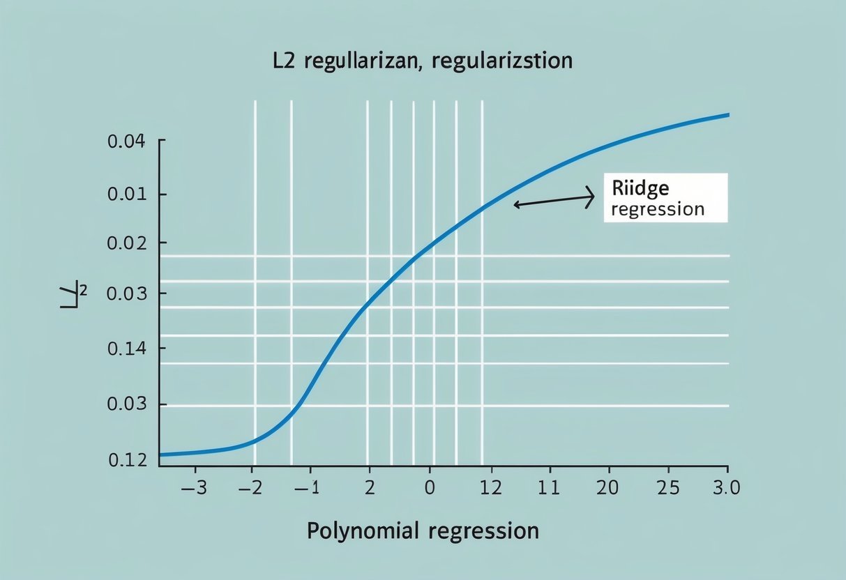
A graph with a curved line representing polynomial regression, with a smaller, smoother line overlaying it to depict the L2 regularization and ridge regression

Applying ridge regression to unseen data requires careful handling to maintain robust predictive performance. This approach helps to prevent overfitting and allows the regression model to generalize well when introduced to new datasets.

Predictive Performance on New Data

When a regression model is exposed to unseen data, how well it predicts is crucial.

Ridge regression introduces a penalty term to handle overfitting by keeping coefficient values small. This regularization helps the model maintain stable predictive performance even with different datasets compared to models without such techniques.

Testing on unseen data provides a realistic measure of how well the model will perform in practical scenarios.

Evaluating ridge regression’s predictive performance often involves comparing R-squared values from training and test datasets. Consistently high values across both suggest the model’s ability to generalize well.

The goal is to ensure the model predicts outcomes accurately across diverse datasets, minimizing errors.

Case Studies and Practical Applications

In real-world applications, ridge regression shows effectiveness in fields such as finance, healthcare, and social sciences.

In finance, it helps in forecasting stock prices by accounting for numerous variables. In healthcare, predicting disease outcomes benefits from the model’s ability to manage multicollinearity in patient data.

Academic studies often demonstrate the advantages of ridge regression. For instance, ridge regression is applied in clinical research to predict patient responses based on multiple factors.

Such case studies emphasize the practical applications of ridge regression for handling complex data with many predictors while maintaining accuracy and interpretability.

Frequently Asked Questions
A chalkboard filled with equations and graphs related to polynomial regression and L2 regularization, with a focus on ridge regression theory

Ridge Regression, a type of L2 regularization, aids in addressing overfitting and multicollinearity issues in regression models. It is distinct from Lasso Regression and has specific applications in machine learning.

What is the purpose of using Ridge Regression in machine learning?

Ridge Regression is used to improve the predictive performance of linear models by adding a penalty for large coefficients, which helps prevent overfitting. This method is particularly useful when dealing with multicollinearity, where independent variables are highly correlated, thereby stabilizing the model.

How does L2 regularization in polynomial regression prevent overfitting?

L2 regularization, also known as Ridge Regression, adds a penalty term to the loss function proportional to the square of the magnitude of coefficients. This discourages complex models by shrinking coefficients, ensuring that the model generalizes better to unseen data rather than capturing noise from the training set.

What distinguishes Ridge Regression from Lasso Regression?

The key difference between Ridge and Lasso Regression lies in their penalty terms. Ridge Regression uses the L2 norm, which shrinks coefficients without setting any to zero. In contrast, Lasso Regression uses the L1 norm, which can shrink some coefficients to zero, effectively performing variable selection.

Can you explain the concept of Ridge Regression and L2 Regularization?

Ridge Regression involves enhancing linear models through L2 regularization, which adds a penalty on the size of coefficients. This helps mitigate issues caused by overfitting and multicollinearity by keeping the model coefficients small, thus leading to more robust predictions and reduced variance in the model’s output.

In what scenarios is Ridge Regression preferred over other types of regression?

Ridge Regression is suitable when dealing with datasets where independent variables are highly correlated, known as multicollinearity. It is also preferred when the goal is to mitigate overfitting without eliminating predictors from the model, making it a reliable choice for complex datasets with numerous predictors.

How is Ridge Regression implemented in programming languages like R?

In R, Ridge Regression can be implemented using packages like glmnet. This package provides functions to fit linear and generalized linear models with regularization paths. This enables the use of Ridge Regression through simple function calls.

Users can specify the regularization strength through the lambda parameter to control the penalty applied to the coefficients.
Categories
Uncategorized

Learn About Defining the Attributes: A Comprehensive Guide

Understanding Attributes

Attributes are essential in distinguishing one concept from another, offering insight into various qualities that define an object or idea.

Definition and Examples

Attributes are inherent qualities or characteristics that identify, describe, or define an object, person, or idea. They act like markers that help to differentiate one thing from another.

For example, in everyday objects, color, size, and shape can all be seen as attributes. In people, attributes might include personality traits such as kindness or creativity. Each attribute helps in forming a complete picture of the subject, offering a deeper understanding of its properties. This understanding is important in fields like education where learner attributes are used to tailor teaching methods, as seen in the Cambridge learner attributes guide.

The Role of Attributes in Classification

Attributes are vital for classification, acting as criteria for grouping similar items together. They provide the basis for categorizing objects or ideas within a system.

For instance, biologists use attributes such as physical features and behaviors to classify animals into species. In computer science, attributes help in database management by defining fields that characterize entries.

Attributes in behavioral analysis, like those discussed in analysis of concepts, are critical for categorizing behaviors under specific stimuli. These qualities ensure a structured approach to understanding complex systems, making them indispensable in various scientific and practical applications.

Types of Attributes

Attributes describe the characteristics or properties of objects or entities. They can be inherent, naturally part of the entity, or acquired through interaction or change. They can also be physical, tangible features, or abstract, representing more intangible qualities.

Inherent vs. Acquired Attributes

Inherent attributes are those characteristics that an object or individual possesses naturally. These are often unchanged over the entity’s life, such as a person’s eye color or the atomic number of an element. These attributes define essential qualities that make an entity unique.

Acquired attributes, on the other hand, are developed or obtained over time. These can include skills learned or behaviors adopted through experience or training.

For example, speaking multiple languages or gaining a new skill set through education. Acquired attributes are significant in adapting to new environments or challenges and often provide a competitive edge.

Physical vs. Abstract Attributes

Physical attributes refer to tangible characteristics that can be observed and measured directly. These include height, weight, color, or texture.

Physical attributes are important in fields like material science, biology, and manufacturing, where precise measurements define quality and functionality.

Abstract attributes are intangible qualities or traits, such as intelligence, bravery, or creativity. These cannot be measured directly but are identified through behavior or performance.

Abstract attributes play a crucial role in fields like psychology and arts, where understanding complex traits helps create better systems or strategies.

Measuring and Identifying Attributes

When measuring and identifying attributes, it’s essential to understand the difference between quantitative and qualitative assessments, as well as the tools and techniques available for accurate measurement.

These methods help categorize and evaluate the various characteristics of an object or data set.

Quantitative vs. Qualitative Assessment

Quantitative assessment involves measuring attributes with numerical values. This type of assessment is used for attributes like length, weight, and volume, which can be measured precisely using units such as meters or kilograms.

Quantitative data provide specific, measurable insights, making it easier to compare different objects effectively.

Qualitative assessment, on the other hand, involves non-numerical evaluation. It focuses on qualities such as color, texture, or taste, where subjective judgment plays a key role.

Descriptions often include terms like “soft,” “bright,” or “flavorful,” which can vary between observers. Qualitative data help in understanding attributes that are hard to quantify directly, providing context and depth to evaluations.

Tools and Techniques for Measurement

Selecting the right tools is crucial for accurate measurement of attributes.

Rulers and scales are commonly used for quantitative measurements, allowing precise determination of size and weight. For assessing length, tools like tape measures and calipers are essential.

These instruments provide accurate and reliable data that support detailed analysis.

In qualitative assessments, techniques such as surveys or interviews can capture subjective attributes. These methods rely on human input to gauge qualities that cannot be measured numerically.

Observation is another technique that gathers data through careful watching and noting of characteristics. These tools and techniques help assess both measurable and non-measurable qualities effectively.

Attributes in Different Contexts

Attributes can refer to defining traits or characteristics in various settings. They play a crucial role in differentiating individuals and shaping organizational identity.

Individuals’ Characteristics

In individuals, attributes are the qualities or traits that define a person’s behavior and thinking. These characteristics include empathy, perseverance, and integrity.

Empathy helps individuals connect with others by understanding their feelings and perspectives. Perseverance is an attribute that drives individuals to overcome challenges and stay committed to their goals, even when facing obstacles. Integrity involves being honest and having strong moral principles, which earns trust from others.

Attributes can significantly shape how people interact with the world around them. They influence personal growth and relationships. Individuals with strong positive attributes are often more successful in various aspects of life, ranging from relationships to professional achievements.

Organizational Qualities

In organizations, attributes refer to the characteristics that define their culture and operational approach. These qualities can include adaptability, innovation, and accountability.

Adaptability allows organizations to remain flexible and responsive to change, ensuring long-term sustainability. An innovative organization is one that constantly seeks new solutions and improvements, fostering a culture of creativity. Accountability involves taking responsibility for actions and decisions, which builds trust among stakeholders.

Understanding these qualities is essential for maintaining a competitive edge in the business environment.

Companies that focus on their key attributes are often better positioned to achieve long-term success and build a strong reputation in their industry.

Organizations that foster positive attributes can create a productive and harmonious work environment, benefiting both employees and clients.

The Significance of Angles in Definition

Angles are fundamental in both geometric and conceptual definitions. Their relevance spans various disciplines, influencing the understanding of physical shapes as well as abstract concepts.

Perspectives in Attribute Analysis

When analyzing attributes, angles provide a clear way to define space and form in geometry. For instance, a triangle’s definition relies heavily on its angles, which determine its type—such as equilateral or isosceles. Accurate measurement is crucial to understanding the nature of these geometric figures.

In problem-solving and mathematics, angles serve as a core concept. They help in calculating distances and establishing relationships between different shapes. Understanding angles aids in better comprehension of spatial attributes, providing insight into the structure and symmetry of figures.

Angles in Physical vs. Conceptual Attributes

In the physical world, angles form the basis of designing structures and objects. Blueprint layouts use precise angles to ensure stability and functionality.

For example, engineering projects rely on angles to determine the load distribution and integrity of constructions.

On a conceptual level, angles influence the interpretation of data and trends. They are pivotal in visual representations like graphs and charts, where they help in visualizing relationships and patterns.

The angles in pie charts, for instance, represent proportions, making complex data more digestible and comparable.

These applications highlight the importance of angles beyond their basic mathematical definition, showcasing their role in bridging the gap between theory and practical use.

Conflict and Attributes

Understanding how attributes affect conflicts is essential. Different characteristics can either worsen disagreements or help resolve them by bringing new perspectives and solutions.

Resolving Conflicting Characteristics

In conflicts, the individual traits people bring can sometimes clash. For example, a team with a mix of assertive and reserved members may face challenges in communication. Assertive individuals might dominate discussions, while reserved members may feel overlooked.

Effective conflict resolution involves recognizing these differences and finding ways to balance them. Techniques like active listening and structured discussions can help create an environment where every attribute is valued.

By encouraging dialogue, teams can harness diverse qualities, turning potential conflicts into opportunities for growth. Emphasizing respect and empathy can reduce misunderstandings, allowing diverse attributes to coexist productively.

Complementary vs. Conflicting Qualities

Attributes can be either complementary or conflicting. Complementary qualities enhance collaboration. For instance, a creative team member paired with a detail-oriented colleague can result in innovative yet practical solutions.

On the other hand, conflicting qualities can lead to tension and disputes. A clash between someone who values quick decision-making and another who prefers thorough analysis can result in frustration.

Recognizing whether attributes are complementary or conflicting helps in managing team dynamics.

Creating strategies that leverage complementary traits can lead to successful outcomes. This approach ensures that all team members feel their unique attributes contribute positively to the group’s goals. Working towards integrating differing qualities fosters a harmonious and effective team environment.

Attributes in Human Behaviors

Attributes in human behaviors include both psychological and sociocultural aspects. These attributes influence how individuals think, feel, and interact within their societies. Understanding these components helps in comprehending human conduct.

Psychological Attributes

Psychological attributes refer to various mental characteristics that drive behavior. These include personality traits like openness, conscientiousness, and extraversion.

Each of these traits affects how people respond to situations and make decisions. For example, a person high in extraversion might seek social gatherings more actively than someone who is introverted.

Emotions are another critical psychological attribute, impacting decision-making and actions. Factors like mood and emotional intelligence determine how one reacts to challenges or opportunities.

Cognitive processes, including perception and memory, also play a significant role in behavioral attributes. These processes shape how information is understood and stored, influencing future actions and attitudes.

Sociocultural Characteristics

Sociocultural characteristics focus on how society and culture influence behavior. Social norms, values, and traditions deeply affect individual actions and social interactions.

For example, collective society members might prioritize group goals over personal achievements, guided by cultural norms.

Roles within society, such as being a parent or a student, come with specific expectations. These roles shape how individuals behave in given contexts.

Cultural attributes also include language and communication styles, which vary widely across different societies. Understanding cultural diversity in behavior helps in acknowledging both differences and commonalities in human conduct.

Social and cultural elements together create a framework within which individual behavior is expressed and interpreted.

Attributes in Science and Technology

A scientist in a lab, surrounded by various scientific equipment and technology, carefully examines and categorizes different attributes

Science and technology each have unique attributes. Scientific research focuses on specific characteristics that define its methods and findings. Technology, meanwhile, emphasizes practical innovation and advancement. Understanding these attributes is crucial for recognizing the impact and development in these fields.

Defining Characteristics in Scientific Research

Scientific research is marked by key characteristics that ensure its rigor and credibility.

Objectivity is essential, as researchers must observe and report facts without bias. This approach guarantees that experiments can be verified and results are reliable.

Precision and accuracy are vital in measurements and data collection, ensuring that findings accurately reflect what is being studied.

Another important characteristic is systematic exploration. Researchers follow structured methods to explore scientific questions, ensuring that investigations follow logical steps.

Ethical neutrality allows scientists to pursue truths without allowing personal beliefs to influence outcomes, maintaining science’s integrity.

Predictability allows researchers to make forecasts based on established scientific principles, demonstrating the dependability of scientific methods.

Attributes of Technological Innovations

Technological innovations focus on applying scientific insights to real-world problems. Innovations aim to improve efficiency and effectiveness in various fields.

They rely on attributes like practicality and usability, making new technologies accessible and beneficial to users.

Adaptability is crucial, allowing technologies to evolve with changing needs and contexts.

Reliability and durability are key attributes of successful technology. Innovations need to perform consistently under different conditions.

Innovation is driven by creativity and the ability to think outside traditional boundaries, leading to breakthroughs that reshape industries.

Qualities in Arts and Design

A colorful palette of paintbrushes, pencils, and markers arranged on a clean, white desk, with a bright window casting natural light onto the tools

Exploring qualities in arts and design includes understanding attributes like balance, color, and texture. These elements work together to create engaging and meaningful compositions.

Artistic Attributes

In art, attributes such as line, shape, and texture play a vital role in creating visual impact.

Lines can guide the viewer’s eye or create movement in a piece. Shapes add structure and form, often defining the overall composition.

Texture gives a sense of depth, whether implied or actual, enhancing the viewer’s tactile experience.

Color is another key attribute. It has three main characteristics: hue, value, and intensity, which determines how light or dark and how bright or dull a color appears.

These color attributes can evoke emotions and set the mood of the artwork. Learning about color can enhance an artist’s ability to convey messages through their work. Explore more about color characteristics at Library Guides on Design Fundamentals.

Design Qualities

Design qualities often focus on usability and aesthetics.

Balance and contrast are important for maintaining visual interest and harmony in a design. Balance creates an even distribution of elements, while contrast highlights differences to draw attention to focal points.

Proportion and scale affect how elements relate to each other and to the space they occupy. This can impact how a design is perceived in terms of importance and readability.

Unity is a quality that ensures all elements of the design work cohesively. This unity can be achieved through repeated patterns or consistent use of color and shape.

These qualities work in tandem to create functional and visually appealing designs that effectively communicate their intended message.

Attributes in Decision-Making

In decision-making, the qualities and attributes individuals or organizations consider can significantly impact their choices and strategic planning. Exploring these aspects helps clarify how decisions are shaped by various factors.

Influence of Qualities on Choices

Attributes play a crucial role in how decisions are made.

Decision-makers often weigh pros and cons by evaluating qualities like effectiveness, cost, and impact. For instance, when a company needs to choose a new supplier, they might assess reliability, product quality, and price.

These attributes can determine the success or failure of the decision, as overlooking them might lead to poor outcomes.

In personal decisions, qualities like convenience and personal value can sway choices. For example, someone choosing a smartphone might prioritize camera quality or battery life based on their own needs. Recognizing which attributes hold the most weight in any given situation is essential for making informed and effective choices.

Attributes and Strategic Planning

Strategic planning relies heavily on understanding important attributes and aligning them with organizational goals.

When planning for the long term, it’s vital to identify attributes that are crucial to achieving objectives. This might include innovation, market position, or customer satisfaction.

Every choice in strategic planning should reflect these attributes to ensure coherence and alignment with the overall vision.

A detailed approach helps organizations prioritize their efforts and allocate resources efficiently. By focusing on the relevant attributes, companies can develop strategies that are more resilient and adaptable to change. This alignment aids in anticipating challenges and leveraging strengths to gain a competitive advantage in the marketplace.

Evolution of Attributes

A tree growing from a small sapling to a mature, sturdy oak, symbolizing the evolution and growth of attributes

Throughout history, human traits have undergone significant changes due to evolutionary pressures and cultural shifts. These changes include adaptations like walking on two legs and the development of language. As we explore these shifts, understanding how these attributes evolved and why some became more important over time is key.

Adaptation and Change of Characteristics

Early humans evolved several key characteristics to survive in their environment.

One notable change is bipedalism, or walking on two legs, which appeared over four million years ago. This adaptation allowed early humans to travel further and use their hands more efficiently.

Another significant evolution was the development of a larger brain, which enabled advanced problem-solving and communication skills. This allowed for the creation and use of tools, which greatly impacted survival rates.

The capacity for developing language is another vital trait that emerged, facilitating complex social interactions and the sharing of information.

These adaptations highlight the dynamic nature of human evolution and how specific traits developed in response to changing environments.

Historical Shifts in Attribute Importance

Over time, some human attributes have gained or lost importance.

During earlier eras, physical traits such as strength and endurance were crucial for survival. As societies evolved, intellectual and social skills began to play a more critical role.

The capacity for ethics became significant as societies formed. This shift marked an important threshold in human evolution, where moral behavior became a defining aspect of humanity.

As communities grew, traits like empathy and cooperation became increasingly valued.

With cultural evolution, human society began placing greater emphasis on intellectual abilities, leading to advancements in technology and culture. These historical shifts underline how the significance of certain attributes can change with societal needs and environmental pressures.

Attributes in Language and Communication

A colorful web of interconnected lines and shapes symbolizing various attributes and communication elements

Attributes in language play a crucial role in shaping how ideas and emotions are conveyed. These attributes not only help in describing and modifying linguistic structures but also enhance effective communication by clarifying qualities and characteristics.

Descriptive Language for Attributes

Descriptive language is pivotal in highlighting attributes within communication. It focuses on adjectives and adverbs that modify nouns or verbs, allowing for more vivid imagery and precise understanding.

By employing descriptive attributes, speakers and writers bring depth to their expressions, enabling listeners or readers to form clear mental images.

For example, referring to a “lush, green forest” instead of just a “forest” provides a richer description. Such details engage the audience and add emotional and visual layers to the communication.

In literature, authors often use descriptive language to create vivid worlds and dynamic characters, making the narrative more engaging. This approach increases relatability and fosters a stronger connection between the communicator and the audience.

Communicating Qualities Effectively

Effectively communicating qualities requires clarity and precision in language use.

Attributes like tone, emphasis, and pacing assist in conveying messages clearly, ensuring that the listener or reader accurately receives the intended meaning.

For instance, a firm tone can communicate confidence, while a softer tone may indicate empathy or kindness.

Utilizing specific language and examples is essential in effective communication.

For example, stating “The project was successful due to innovative planning and diligent execution” highlights particular qualities that contributed to the outcome. This approach ensures that the strengths and characteristics of subjects are communicated without ambiguity.

Attention to such details enhances understanding and allows the communicator to convey the message more convincingly and succinctly.

Frequently Asked Questions

A stack of open books with question marks floating above them

Attributes are an essential part of many fields, like computer science and programming languages. They define characteristics of HTML elements, objects in JavaScript, and more.

What is the process for defining attributes in HTML elements?

In HTML, attributes provide more information about elements.

Attributes like href for links, src for images, and class or id for styling are common. They are specified in the opening tag of an element, often in the form of attribute="value".

How do attributes function in JavaScript objects?

JavaScript objects are made up of properties, which are attributes that have name-value pairs.

These attributes can store different types of data, such as numbers, strings, and functions, allowing objects to have specific behaviors and characteristics.

Can you provide some examples of attributes in computer science?

In computer science, attributes can refer to aspects of data structures.

For example, an Entity-Relationship model uses attributes to describe properties of an entity, like a student with attributes such as name, age, and roll number, which can be found in ER models.

What are some common attributes of geometric shapes?

Geometric shapes have attributes that define their properties. These can include the number of sides, angles, area, and perimeter.

For example, a circle’s attributes would include its radius and diameter, while a rectangle has length and width.

How are attributes used in C# programming?

In C#, attributes are used to add metadata to code elements like classes and methods.

Attributes can specify information such as serialization details or mark methods with specific behaviors or roles, thereby enhancing functionality and usability.

What are typical personal attributes that individuals possess?

Personal attributes refer to traits or qualities that define a person. Common attributes include honesty, kindness, patience, adaptability, and persistence.

These attributes are often considered key components of an individual’s character and personality.

Categories
Uncategorized

Learning Pandas for Data Science – Mastering Apply(), Map(), and Applymap() Functions

Understanding Pandas in Data Science

Pandas is a key library in Python that supports data manipulation and analysis. It offers two essential data structures: DataFrame and Series.

These are critical for efficiently handling and processing large datasets, allowing users to perform a variety of operations with ease.

Key Components of Pandas

Pandas is built around two primary components: DataFrame and Series.

A DataFrame is a two-dimensional, size-mutable, and potentially heterogeneous data structure with labeled axes. It is comparable to a table in a database or a data frame in R.

Users can easily perform operations such as filtering, grouping, and transforming data. The power of DataFrame lies in its ability to operate with large amounts of data quickly.

A Series is a one-dimensional array holding data of any type. It operates similarly to a list in Python but comes with indices, making it easier to track data.

It can also be used to apply functions to subsets of data, offering a flexible approach to data handling. This robust component allows for seamless data manipulation and is essential for data preprocessing.

Data Structures: DataFrame and Series

The DataFrame structure is composed of rows and columns, allowing complex data operations. Each column in a DataFrame can be of a different data type.

This structure is essential for operations like merging, joining, and reshaping data. It also supports arithmetic operations and broadcasting, making numerical data processing efficient.

The Series functions as the foundational structure for creating DataFrames. It has a strong connection with NumPy arrays, supporting all major data operations.

This makes it invaluable for statistical analysis and machine learning tasks, where quick data processing is needed. The indexing capabilities of Series are essential for data alignment, offering a straightforward way to organize and manipulate data.

Principles of Data Transformation

Data transformation is a key process in data science. It involves converting data from one format or structure into another.

This can include element-wise operations, where changes are made to individual data points, and column-wise transformations, focusing on entire columns or features of a dataset.

Common transformations are often done using Pandas in Python. Functions like apply(), map(), and applymap() are helpful.

apply() can perform transformations on a whole row or column, while map() is used for substituting each value in a series with another value.

applymap() is specifically designed for element-wise operations on data frames, allowing changes at the level of individual elements.

Basic Operations

Some basic transformations include arithmetic operations such as addition, subtraction, multiplication, and division.

For example, adding a constant value to a column or dividing all elements in a data frame by a specific number is common in preprocessing.

import pandas as pd
# Example of adding a constant value to a column
df['column'] += 10

Use Cases

Element-wise transformations are typically used for cleaning data or making adjustments based on certain conditions.

Column-wise transformations often prepare data for analysis by normalizing or scaling data. This ensures that data is in a suitable form for machine learning models.

Introduction to User Defined Functions

User defined functions in Python are essential for performing specific tasks repeatedly without rewriting code. They enhance code readability and reusability. This section will explore how functions serve as callable entities and the role of callable objects in Python programming.

Understanding Functions in Python

In Python, a function is a block of organized, reusable code that performs a single task. Functions are defined using the def keyword, followed by a name and parentheses () that may contain parameters.

The code block within the function is indented and executed when the function is called.

Python allows for flexibility in functions by accepting different types of parameters, such as positional, keyword, and default. Functions can return results using the return statement, which ends the function’s execution.

A simple example:

def greet():
    print("Hello, world!")

Functions can aid in reducing redundancy, making it easier to manage large-scale projects. They also promote modularity by segmenting different operations within code.

Role of Callable Objects

Callable objects are entities in Python that can be called like functions. They include functions, methods, and classes with a __call__ method.

Callable objects provide a great deal of flexibility and power in Python programming.

Using callable objects, developers can implement complex behaviors by defining custom logic within classes. This allows for objects to act like functions and maintain internal states, which can be handy in numerous programming scenarios.

For example, Python’s built-in map() and filter() functions take other functions as arguments, showcasing how callable objects enhance code efficiency and functionality.

Callable objects also align with Python’s functional programming style, promoting cleaner and more concise code.

Employing Apply() for DataFrames

In the world of data science, the apply() function in pandas is essential for performing operations on DataFrames, enabling customization and efficiency. Through this function, users can execute complex operations either row-wise or column-wise.

Basics of Apply()

The apply() function in pandas is versatile for working with DataFrames. It allows users to perform custom operations by applying a function along an axis.

The use of dataframe.apply() can handle both row and column-wise operations by specifying the axis parameter.

Syntax:

dataframe.apply(func, axis=0)

Here, func is the function applied, and axis=0 applies it column-wise, while axis=1 applies it row-wise.

One common use is applying lambda functions for transformations or calculations that aren’t directly supported by pandas’ built-in methods.

This makes apply() a powerful tool for data manipulation and cleaning tasks, enhancing the flexibility of a pandas DataFrame.

Advanced Apply() Techniques

For more advanced uses, apply() can be combined with other features like series or even return custom objects.

Using apply() with user-defined functions maximizes performance and tailored computations.

By leveraging these techniques, complex conditional logic can be introduced to columns, or aggregates can be calculated.

Example:
Grouping similar tasks:

def complex_function(row):
    # Perform operations
    return result

dataframe['new_column'] = dataframe.apply(complex_function, axis=1)

This example highlights apply()‘s role in enabling sophisticated manipulations without the need for looping. For tasks like modifying data based on conditional logic across columns, apply() ensures both precision and clarity, crucial for large datasets.

Leveraging Map() for Series Objects

Map() is a powerful tool in Pandas, helping users change Series data by applying a function or replacing values with a dictionary. This method offers flexibility and efficiency, making it ideal for data cleaning and transformation tasks.

Understanding Map()

The map() function is used with Pandas Series objects to streamline data changes. By applying map(), each element in a Series can be transformed using a specified function or replaced with a corresponding value from a dictionary.

This capability is particularly useful for data preprocessing, where specific values need to be modified systematically.

For instance, consider a Series of categorical values that need to be converted into numeric codes. Using a dictionary with map(), the transformation can be executed efficiently. This technique eliminates the need for loops, offering a more concise and readable approach to data manipulation.

Mapping with Functions and Dictionaries

One of the strengths of map() is its ability to utilize both functions and dictionaries.

When a function is used, it is applied to each element of the Series, enabling customization and transformation based on specific rules.

Alternatively, leveraging a dictionary allows for direct substitution of values.

For example, a dictionary might map ‘cat’ to 1 and ‘dog’ to 2, effortlessly transforming text data into numerical format.

These features make map() a versatile tool in data science, simplifying complex operations and enhancing the efficiency of tasks such as data cleaning and feature engineering.

Utilizing Applymap() for Element-wise Operations

The applymap() function in Pandas is a powerful tool used for performing element-wise operations on all entries of a DataFrame. It is particularly useful when you need to apply a function to each individual element, such as handling missing values or transforming data types.

Basics of Applymap()

The applymap() function is specifically designed for DataFrames. It applies a given function to every single element in the DataFrame, which distinguishes it from the apply() method that works on rows or columns.

For instance, to convert all values to integers, one might use dataframe.applymap(int). This operation ensures consistency across the DataFrame’s elements.

Unlike apply(), which processes entire rows or columns, applymap() can directly manipulate each cell.

Handling missing values or NaN values is another area where applymap() shines. By applying a function that checks and replaces NaN, users can clean their data efficiently.

This function is also handy for formatting strings or numerical data as per the requirement of your analysis.

Error Handling in User Defined Functions

Error handling in user-defined functions is crucial for maintaining robust data analysis processes.

When working with Pandas functions like apply(), map(), and applymap(), handling errors such as TypeError and managing NaN values are key challenges.

Understanding and effectively managing these errors can help prevent unexpected results and interruptions in data processing.

Managing TypeError

A TypeError often arises when an operation is performed on an unsupported data type. In user-defined functions, this error might occur if the input data type does not match the expected type in operations.

The function should include checks and validations to ensure data types are as expected before processing.

Using try-except blocks is a common approach for catching TypeError. This allows the function to continue running smoothly even if an incorrect data type is encountered.

Additionally, logging the error can be helpful for debugging and understanding which data points are causing issues. Knowing where and why these errors occur is key to refining the overall data handling process.

Dealing with NaN and Missing Values

NaN values are prevalent in datasets and can disrupt calculations and analyses if not handled correctly.

In Pandas, user-defined functions must address these missing values to maintain the integrity of data processing.

Strategies such as skipping, filling, or removing NaN values can be applied based on the specific requirements of the analysis.

Pandas provides methods like fillna() for replacing NaN with specified values, and dropna() to remove these entries altogether.

The choice between these methods depends on the data context and the importance of missing values to the analysis.

Proper handling of missing data points ensures that the results remain accurate and reliable.

Optimizing Performance with UDFs

Optimizing the performance of User Defined Functions (UDFs) in pandas is crucial for large data processing tasks. Understanding the techniques like benchmarking and vectorization with NumPy can lead to significant speed enhancements.

Benchmarking UDF Performance

Benchmarking is a method used to measure the performance of UDFs. It helps in identifying bottlenecks in code execution.

By using tools like %timeit in Jupyter Notebook, one can effectively track the execution time of UDFs.

Performance analysis can be broken down with statistical tables displaying averages, minimums, and maximum execution times.

Adjusting UDFs based on benchmarking results helps in refining functions to run more efficiently.

For instance, optimizing loops or reducing function calls can decrease latency.

Careful benchmarking sets the stage for more advanced optimizations.

Vectorization with NumPy

Vectorization with NumPy is another powerful optimization technique. It allows replacing explicit loops with array operations, which are generally faster.

NumPy’s operations are implemented in C, making them more efficient than regular Python loops.

Instead of applying UDFs row by row, leveraging NumPy’s vectorized functions can significantly boost performance.

For example, instead of using a loop to add two arrays element-wise, use numpy.add(). This reduces overhead and speeds up computations.

Adopting vectorization where possible in code results in cleaner and faster-performing data manipulation tasks.

Mastering Lambda Functions in Pandas

Lambda functions offer a concise way to create anonymous functions in Python. In Pandas, these are often used to manipulate or transform data in flexible and efficient ways.

The Basics of Lambda Expressions

Lambda expressions in Python are small, anonymous functions defined with the lambda keyword. They allow the creation of simple functions without formally defining them using def.

These expressions take any number of arguments but have only one expression. In Pandas, lambda functions are often utilized for quick transformations or computations on DataFrame objects.

For example, a simple lambda expression can square a number:

square = lambda x: x * x

Pandas takes advantage of this flexibility, enabling users to apply transformations directly to DataFrame columns.

Integrating Lambda with Apply, Map, and Applymap

In Pandas, lambda functions are frequently paired with apply(), map(), and applymap() to perform operations.

The apply() function is used to apply a function along an axis of the DataFrame, enabling operations on either rows or columns.

df['column'].apply(lambda x: x + 1)

The map() function is ideal for transforming each element in a Series using a function. This method is useful for mapping values or performing element-wise operations.

df['column'] = df['column'].map(lambda x: x.title())

Applymap() works on every element of the DataFrame, making it suitable for element-wise transformations across a full dataset.

df.applymap(lambda x: x * 2)

By integrating lambda functions with these Pandas methods, users can efficiently conduct complex data manipulations.

Appending Data to DataFrames

A person using a computer to manipulate data in a spreadsheet using Python's Pandas library

Adding data to DataFrames in Pandas involves two main techniques: simple addition and using apply functions. Each method serves different needs depending on the complexity of data operations required.

Simple Addition to DataFrames

The most straightforward way to append data to a DataFrame is by using the append() method or concat() function. These allow new rows to be added cleanly.

For example, using df.append(new_row) integrates a new record effortlessly.

You can also use concat() for merging multiple DataFrames. This is especially useful for combining large data sets with consistent columns.

For instance, pd.concat([df1, df2]) will create a new DataFrame from the two original ones. This method is reliable for combining structured data.

Advantages of these methods include ease of use and preserving the original order of the columns. However, it’s important to ensure that the data types of the appended rows match those in the existing DataFrame to prevent errors.

Appending Data with Apply Functions

Using apply functions provides more advanced ways to append data based on specific conditions or calculations.

The apply() function can help manipulate and transform data before appending. For example, it can run transformations on each row, allowing complex operations like normalizing values or computing new metrics before adding them to the DataFrame.

The applymap() function is suitable for element-wise operations across the DataFrame. For instance, it can be used to apply a mathematical operation to each element within a DataFrame, such as multiplying each element by a constant.

These functions offer flexibility in data manipulation and can handle diverse requirements. While they add complexity, their use ensures that appended data is processed and integrated logically.

Practical Examples of UDFs in Action

User-defined functions (UDFs) in Pandas, such as apply(), map(), and applymap(), are crucial tools that enhance data manipulation. These functions help in transforming and analyzing data sets efficiently.

Real-world Examples of Apply()

The apply() function is highly versatile and can be used to manipulate data in rows or columns.

Consider a data set with sales data. A retailer might want to calculate taxes on each sale. Using apply(), this task becomes straightforward. They can define a function for tax calculation and use apply() to execute this function across the relevant column.

Another practical example is cleaning data. Suppose there’s a column with mixed data types, possibly causing errors in analysis. A custom function can be designed to standardize these values.

By implementing apply(), the function processes each entry quickly, ensuring consistency and reliability across the data set.

Case Studies Using Map and Applymap

The map() function is often used to transform data by mapping existing values to new ones. For instance, converting gender labels from “M” and “F” to “Male” and “Female” is a common task.

By creating a dictionary of mappings and applying map() to the relevant column, data transformation is efficiently managed.

In contrast, applymap() is useful for element-wise operations across an entire DataFrame.

Consider a case where a data set contains prices that need to be converted from one currency to another. A function to perform this conversion can be applied across the DataFrame using applymap(). This ensures all elements are adjusted, maintaining data uniformity and accuracy.

Comprehending UDF Syntax and Structure

Understanding the syntax and structure of User Defined Functions (UDFs) in Pandas is crucial for efficient data manipulation. This involves utilizing functions like apply(), map(), and applymap(), each serving unique purposes in data transformation.

Anatomy of a UDF

A User Defined Function (UDF) is a function written to perform specific operations that are not available with built-in functions.

In Pandas, UDFs are often used to apply custom calculations on data series or DataFrame columns.

The basic anatomy of a UDF includes a clear function definition using the def keyword, input parameters (typically data rows or values), and a return statement that outputs the desired result after applying the function logic.

By leveraging UDFs in data processing, users enhance the flexibility and power of data transformations.

Syntax Details for Apply, Map, and Applymap

The apply() function is versatile, enabling row-wise or column-wise operations on a DataFrame. An example syntax is df.apply(func, axis=0), where func is the UDF and axis determines the application direction (0 for columns, 1 for rows).

The map() function is used with Series, allowing element-wise operations. The syntax series.map(func) applies the UDF to each element of the Series.

applymap() specifically targets DataFrame elements individually. It is beneficial for altering each value in a DataFrame and is utilized as df.applymap(func).

These functions offer tailored control over data processing, expanding Python’s toolkit for handling diverse datasets.

Frequently Asked Questions

Pandas offers several powerful methods for data manipulation. Among them, apply(), map(), and applymap() each have unique uses and performance characteristics. Understanding when and how to use these functions is key for efficient data processing.

How do the performance characteristics of Pandas apply() and map() differ in data manipulation?

apply() is versatile and works on both DataFrames and Series. It can handle more complex functions but may be slower.

The map() function is applied to Series and is generally faster for element-wise operations because it’s more specific and optimized for simpler tasks.

What are the use cases for the applymap() function in Pandas?

The applymap() function is specifically designed for element-wise operations on DataFrames. It applies the same function to every element in the DataFrame. This makes it useful for tasks like cleaning data, where the same transformation is needed across all elements.

In what scenarios should I use apply() over map() or applymap() when working with Pandas?

apply() should be used when complex operations need to be performed across an entire axis of a DataFrame.

It is ideal for row-wise or column-wise calculations and can apply functions that require more context or involve more logic than simple element-wise operations.

Has the applymap() function in Pandas been deprecated and if so, what alternatives exist?

As of the current information, applymap() has not been deprecated in Pandas and remains a viable option for element-wise DataFrame operations.

While there are no direct alternatives, manual element-wise operations using loops or vectorized NumPy functions can sometimes serve similar purposes.

Could you provide an example of how to use the map() function with a dictionary in Pandas?

The map() function can replace Series values using a dictionary. For example, if there is a Series of city codes, map() can replace each code with its corresponding city name from a dictionary.

This makes it a useful tool for value mapping and transformation.

When should the Series apply() method be utilized in Pandas instead of map() or applymap()?

The Series apply() method is preferable. It is used when a function involving logic or computation needs to be applied to each element. It offers more flexibility than map() because it can handle more complex scenarios. For example, it can apply lambda functions or built-in methods that require multiple operations.

Categories
Uncategorized

Learning Advanced Python Skills for Data Engineering: A Comprehensive Guide

Python Fundamentals

Understanding Python’s fundamentals is essential for mastering more advanced data engineering tasks.

Key components include basic syntax, managing data using variables, decision-making with control structures, and working with essential collections like lists and dictionaries.

Language Basics

Python is known for its clean and readable syntax, making it a popular choice for beginners and experts alike. The language uses indentation to define the structure of the code, which is crucial for functions, loops, and conditionals.

Learning how to implement these elements correctly is foundational.

Comments are also necessary for explaining code sections. They are added with the # symbol, helping programmers understand and maintain the code over time.

The simplicity of Python syntax reduces errors and enhances code readability, a significant advantage in data engineering where complexity is common.

Consistent practice with foundational syntax will improve fluency and efficiency in writing Python code.

Variables and Data Types

Variables in Python serve as containers for storing data values. They can hold various data types, such as integers, floats, and strings, each suited for specific roles in data operations.

Variable Declaration is simple and doesn’t require explicit type definition. For instance, name = "Data Engineer" creates a string, while age = 30 creates an integer. This flexibility encourages experimentation and ease of use.

Understanding data types like integers, floats, and strings is vital.

Lists are used for holding ordered collections of items, whereas dictionaries store key-value pairs. These structures allow efficient data manipulation, which is crucial in building and managing data pipelines.

Control Structures

Control structures are essential for directing the flow of a Python program.

Conditional statements, such as if, elif, and else, allow programs to make decisions based on conditions.

Loops, specifically for and while loops, are utilized to repeat actions until certain criteria are met. This is particularly useful for processing large data sets in data engineering.

Mastering these control structures allows programmers to automate and streamline repetitive tasks, enhancing productivity.

Control structures are central for developing complex algorithms that perform a wide range of data processing tasks efficiently.

Python Collections

Python collections are versatile tools for storing and manipulating groups of data. Key collections include lists, tuples, sets, and dictionaries, each with unique characteristics.

  • Lists are ordered and mutable, making them ideal for dynamic collections.
  • Tuples are ordered and immutable, preserving data integrity.
  • Sets store unordered, unique items, useful for removing duplicates.
  • Dictionaries offer key-value pairing, which is handy for rapid data retrieval.

Understanding these collections allows engineers to handle complex data coordination.

Knowing when and how to use each type ensures optimized and efficient code when dealing with large volumes of data. Each collection type has its specific functions, making them versatile for various tasks in data processing and management.

Object-Oriented Programming in Python

Object-oriented programming (OOP) is a core aspect of Python programming that enhances coding skills for data engineering. Key concepts include defining classes, utilizing inheritance and polymorphism, and implementing encapsulation and abstraction.

Defining Classes

In Python programming, classes serve as blueprints for creating objects. They encapsulate both data (attributes) and functions (methods) that operate on that data. This tool allows developers to structure their code by partitioning data and behavior.

A basic class structure includes a __init__ method, which initializes the object’s attributes. For instance, defining a class Car involves specifying its make, model, and year. The __init__ method then sets these attributes when a new Car object is instantiated.

Effective use of classes can simplify code management and improve clarity.

Inheritance and Polymorphism

Inheritance enables a class to derive from another, promoting code reuse and efficiency. In Python, a child class inherits attributes and methods from a parent class, while also introducing unique features.

For example, a Vehicle class might serve as a parent to Car and Bike, allowing shared properties like speed, yet offering specific functions such as honk() for Car. Polymorphism allows these classes to redefine methods as necessary, enabling flexible and dynamic code behavior.

Polymorphism further ensures that a single interface can handle different data types, adding versatility to code by allowing objects to be treated as instances of their parent class.

Encapsulation and Abstraction

Encapsulation in coding skills emphasizes restricting direct access to certain attributes and methods to ensure controlled interaction. In Python, this is often done using private variables, marked by a leading underscore (e.g., _engine). Encapsulation preserves the internal state of an object, safeguarding it against unauthorized modification.

Abstraction simplifies complexity by hiding unnecessary details from the user. Through abstraction, Python developers expose only relevant parts of an object to the outside world. This is typically achieved by defining public methods that provide an interface to interact with data.

Together, encapsulation and abstraction enhance the security and usability of Python programs.

Advanced Python Libraries

Advanced Python libraries play a crucial role in data engineering tasks, facilitating efficient data handling and numerical computations. Among these, Pandas and NumPy are renowned for their capabilities and ease of use.

Data Handling With Pandas

Pandas is a powerful tool for data manipulation and analysis. It is especially useful for handling structured data. It provides data structures like DataFrames that allow users to manipulate data effortlessly. With its various functionalities, Pandas simplifies tasks such as data cleaning, filtering, and transformation.

Data engineers often use Pandas for tasks involving large datasets. The library supports operations like grouping and merging data, which are essential for preparing datasets for analysis. Its intuitive syntax makes it accessible for quick explorations and in-depth data investigations.

Pandas also integrates well with other libraries used in data engineering, offering compatibility that enhances its utility. Whether aggregating data or conducting exploratory data analysis, Pandas remains a preferred choice for its robust performance.

Numerical Computing With NumPy

NumPy is a foundational library in Python, crucial for numerical computing. It is particularly noted for its array objects that allow efficient storage and manipulation of data. NumPy arrays are faster and more compact than Python lists, making them ideal for numerical tasks.

Data engineers use NumPy for performing complex mathematical operations. Its functions enable high-speed computations required for large-scale data engineering tasks. This is achieved by providing built-in support for large matrices and multidimensional data, which are common in various applications.

The library works seamlessly with other Python libraries, forming the backbone for advanced operations in data engineering and scientific computing. With tools for linear algebra, random number generation, and more, NumPy is indispensable for engineers who require precise and quick computational solutions.

Data Engineering Essentials

A computer screen displaying code in Python, surrounded by data engineering tools and resources

Data engineering involves working with various technologies and tools to manage and process data efficiently. This includes handling databases, creating data pipelines, and performing file operations like reading and writing data.

Working With Databases

In data engineering, databases are crucial for storing and retrieving large amounts of data. Engineers must understand SQL to interact with relational databases and NoSQL for non-relational data storage. These skills help in executing complex queries, data modeling, and indexing.

Databases like MySQL, PostgreSQL, and MongoDB provide versatile options for different data operations. Knowledge of database management systems (DBMS) is also important for ensuring data integrity, security, and performance optimization.

Data Pipelines Fundamentals

A data pipeline is a series of processes used to automate the flow and transformation of data. Understanding ETL (Extract, Transform, Load) is vital for designing effective pipelines.

Tools like Apache Spark and Apache Airflow help in creating scalable and efficient pipelines. Engineers should be proficient in handling big data platforms like Hadoop.

Pipelines enable the processing of real-time data, which is essential for timely insights and decision-making. Engineers must also focus on error handling and monitoring to maintain data quality.

File Handling and I/O Operations

File handling is essential for working with different data formats such as JSON and CSV. Engineers need to handle files for both input and output operations.

They often use Python for its libraries like pandas and NumPy, which simplify data manipulation. Understanding file paths, directories, and how to handle large files efficiently is important.

Techniques like file compression and buffering improve performance and resource management. These skills are critical when dealing with massive datasets typical in large-scale data engineering projects.

Building and Maintaining Data Pipelines

Data pipelines are essential for moving data efficiently across systems. They involve extracting data, transforming it into useful formats, and loading it where needed. This section covers key areas in managing these pipelines: ETL processes, data transformation techniques, and pipeline orchestration.

ETL Processes

ETL stands for Extract, Transform, Load. It is a core component of data pipelines.

The extraction phase pulls data from various sources, such as databases or APIs. This raw data can often be messy or incomplete.

During transformation, the data is cleaned, formatted, and modified to suit specific needs or standards.

As data engineers transform data, they often use programming languages like Python or SQL. These languages help to automate transformations and ensure data quality.

Finally, the load process involves importing the transformed data into a destination system. This could be a data warehouse or an analytics platform, where the data is ready for further analysis.

Successful ETL processes ensure reliable and timely data flow across systems.

Data Transformation Techniques

Data transformation is crucial in a pipeline. It involves converting raw data into a structured format.

Techniques range from basic operations like filtering and sorting to more complex ones like aggregating and joining data from different sources.

Python libraries such as Pandas and NumPy are often used to handle these tasks efficiently. They offer functions to manipulate large datasets with ease.

Additionally, transformations may involve handling missing values and outliers. These steps ensure that data is consistent and accurate.

Advanced transformation techniques might include creating calculated fields or standardizing formats. By doing this, the data becomes more useful and aligns with business goals.

Understanding these techniques facilitates robust data processing and allows clearer insights.

Pipeline Orchestration

Pipeline orchestration involves managing and scheduling data pipeline processes. This is essential for timely data delivery and ensuring processes run in the correct order.

Tools like Apache Airflow or Luigi are commonly used for this purpose. They help automate and monitor workflows efficiently.

Using these tools, engineers can define dependencies between different tasks. For example, a transformation task might need to complete before loading data.

Orchestration ensures all tasks are executed and monitored seamlessly.

By organizing the pipeline workflow, businesses can avoid data bottlenecks and improve efficiency. This reliability is crucial for making data-driven decisions.

Proper orchestration also includes error handling, ensuring that any issues are quickly identified and resolved.

Data Storage and Retrieval

A computer screen displaying code for data storage and retrieval using Python

Understanding how to store and retrieve data efficiently is crucial for data engineering. This area focuses on systems that handle different types of data, including relational databases and NoSQL solutions. Each type offers distinct advantages for scaling and maintaining data processes.

Relational Databases

Relational databases use structured query language (SQL) to store and manage data in rows and columns. They are well-suited for structured data that needs to be consistent and reliable.

Common examples include MySQL, PostgreSQL, and Oracle Database.

Relational databases are essential for applications requiring complex transactions and queries. They support features like ACID compliance, which ensures that all transactions are processed reliably.

These databases can efficiently handle large volumes of data and are often used in banking, telecommunications, and e-commerce.

Normalization is a key concept, ensuring that data is efficiently organized to minimize redundancy. This process helps maintain data integrity.

Relational databases are ideal for use cases where data relationships are crucial, and where data integrity is a priority.

NoSQL and Big Data Solutions

NoSQL databases are designed to handle unstructured data and large datasets. They are ideal for applications where relational databases may not perform efficiently.

NoSQL solutions include MongoDB, Cassandra, and Couchbase. These databases offer flexibility in data models, supporting document, key-value, column-family, and graph models.

This flexibility makes them suitable for applications with rapidly changing requirements, like social media platforms.

NoSQL databases are often used in combination with big data tools like Apache Spark. These tools enable data engineers to process and analyze vast amounts of data efficiently.

With the ability to scale horizontally, NoSQL solutions handle massive data traffic smoothly, making them essential for enterprises dealing with big data challenges and real-time analytics.

Leveraging Cloud Technologies

A computer screen displaying Python code with cloud icons and data engineering symbols

Cloud technologies are vital for modern data engineering, offering scalable and flexible solutions. They help in efficiently managing data pipelines and reducing infrastructure costs.

Cloud Solutions for Data Engineering

Cloud solutions are transforming data engineering by providing robust platforms like Google Cloud, AWS, and Microsoft Azure. These platforms offer a wide range of tools to build, deploy, and manage data pipelines effectively.

Big data processing frameworks such as Apache Spark or Hadoop run smoothly on cloud environments, ensuring scalability and performance.

Data engineers often use these cloud platforms to set up ETL processes, store large datasets, and run analytics effectively. This enables organizations to process complex data workflows without worrying about physical infrastructure limitations.

Advantages of Cloud-Based Data Pipelines

Cloud-based data pipelines offer numerous advantages, making them a preferred choice for data engineers.

One significant benefit is scalability. Cloud platforms can easily handle increasing data volumes without requiring additional hardware. They provide on-demand resources, ensuring cost-effective scalability.

Another advantage is flexibility. Cloud platforms support various data handling tools and programming languages, such as Python and SQL, making it easier to integrate them into existing systems.

This allows data engineers to quickly adapt to changing project requirements and technological advancements.

Finally, cloud-based pipelines ensure reliability by offering high availability and robust security measures, protecting data integrity and privacy. This helps organizations maintain a competitive edge by ensuring that their data infrastructure is both secure and efficient.

Automating Data Engineering Tasks

Automating data engineering tasks can significantly enhance efficiency and reduce manual errors. By employing coding skills in scripting, engineers can set up processes to run seamlessly.

Scheduling these jobs ensures they occur at optimal times, elevating productivity.

Scripting and Automation

Scripting is vital for automating repetitive data tasks. Engineers use programming languages like Python to write scripts that handle data extraction, transformation, and loading (ETL).

These scripts can manage large datasets efficiently, performing operations such as data cleaning and format conversion.

Python libraries such as Pandas and NumPy are popular for manipulating data within scripts. Leveraging the power of scripts reduces the manual workload and mitigates errors.

This allows engineers to focus on more complex data challenges, enhancing overall data pipeline efficiency.

Scheduling Jobs

Scheduling jobs ensures that automated tasks run at specific times or intervals. Tools like Apache Airflow and Cron are often used for this purpose.

Airflow, for instance, provides a detailed user interface to manage complex workflows visually, adding flexibility to task management.

Engineers set parameters for task frequency, such as hourly or daily, to suit the needs of the project. With these scheduling tools, data pipelines are kept up-to-date without manual intervention.

This reliability is crucial in environments where data insights must be fresh and accurate for decision-making.

Real-World Data Engineering Projects

Engaging in real-world data engineering projects is crucial for gaining practical experience and improving problem-solving skills. This section explores hands-on projects aimed at analyzing retail sales data and developing comprehensive capstone projects.

Retail Sales Data Analysis

Retail sales analysis projects provide an opportunity to work with diverse datasets. Participants can learn to manage large volumes of transaction data, track sales trends, and generate insights.

Key tasks involve cleaning and transforming raw data to ensure accuracy.

Analyzing sales records from multiple stores or channels is a valuable exercise in building data pipelines. Python and libraries like Pandas and NumPy are essential tools.

Using Airflow for scheduling and automating data tasks enhances efficiency.

Creating visualizations with Matplotlib or Tableau helps present findings clearly. This project helps develop skills in database management, SQL, and data visualization.

Capstone Project Development

Capstone projects challenge participants to apply everything they’ve learned. These projects often span months and encompass data collection, transformation, and visualization.

A comprehensive capstone project could involve constructing a data pipeline handling real-time data flows.

It’s essential to identify a meaningful problem or use case, then devise a solution using advanced Python techniques.

These projects often require crafting custom scripts for automation.

Working in teams is beneficial for large-scale projects. Collaboration can mirror workplace dynamics, helping participants refine both technical and soft skills.

A successful capstone project can significantly enhance a portfolio, demonstrating a mastery of data engineering concepts.

Integrating Machine Learning Workflows

A computer with multiple screens displaying code, data visualizations, and machine learning algorithms. A bookshelf filled with Python programming books in the background

Integrating machine learning workflows involves preparing data effectively and deploying models for practical use. Key steps include data cleaning, feature selection, and utilizing platforms for model deployment.

Data Preparation for ML

Effective data preparation is critical to the success of machine learning models. It involves cleaning the data to remove noise and inconsistencies.

This step may utilize Python libraries such as Pandas and NumPy for efficient data manipulation.

Feature selection is another vital task, where important variables are chosen to improve model accuracy and performance. These variables help in creating a robust model that generalizes well to unseen data.

Handling missing data is also a part of this process. Imputation techniques or removing incomplete rows might be needed to ensure the dataset is ready for analysis.

Once the data is clean, scaling and transformation techniques prepare it for machine learning algorithms. This creates a dataset that is not only clean but also enhances learning and prediction strength.

Operationalizing ML Models

Operationalizing machine learning models means taking them from development to production. This step ensures that models are not just accurate but also scalable and maintainable.

Using tools like Apache Airflow or MLflow helps automate workflows and manage machine learning lifecycle stages efficiently.

These tools enable version control, tracking of experiments, and environment management, ensuring smooth transition from training to deployment.

Kubernetes and Docker can be employed for containerization, making deployment less complex and more portable across platforms.

Setting up continuous integration and continuous deployment (CI/CD) pipelines allows for seamless updates and monitoring.

This approach minimizes downtime and ensures the models remain effective and current over time, keeping up with changing data patterns and business needs.

Professional Growth in Data Engineering

A person studying a book on advanced Python, surrounded by data engineering tools and resources

To grow in data engineering, professionals should focus on building a strong portfolio and engaging in effective networking. Highlighting skills through well-organized projects and leveraging platforms like LinkedIn can help in standing out. Networking plays a crucial role in finding opportunities and connecting with industry experts.

Building a Strong Portfolio

A compelling portfolio showcases a data engineer’s skills and achievements. Including projects that demonstrate expertise in programming languages and data handling tools is essential.

For instance, a well-documented project using Python for data engineering illustrates proficiency.

Adding case studies with clear objectives and results can make the portfolio more attractive. Certificates from platforms like Coursera support credibility and highlight continued education efforts.

Using a variety of media such as code snippets, visualizations, and project narratives gives a comprehensive view of skills.

LinkedIn and Networking

Networking is a key component in professional growth. A LinkedIn profile acts as a digital resume, helping to connect with peers and industry leaders.

Keeping profiles updated with recent projects and skills improves visibility.

Engaging with groups and discussion forums on LinkedIn can open new opportunities and provide industry insights. Reaching out to connections for informational interviews helps in gaining deeper understanding and advice from experienced professionals.

Attending webinars and seminars expands knowledge and offers chances to meet potential employers.

Building a strong network fosters collaboration and opens doors to various career advancements.

Certification and Continuing Education

A computer screen displaying Python code with a certification and continuing education logo in the background

Data engineering is a rapidly evolving field, and gaining recognized certifications can give professionals a significant edge. Continuing education is key for staying current and competitive. This section covers certifications as well as strategies for lifelong learning.

Gaining Recognized Certifications

Earning certifications such as the Professional Certificate in Data Engineering can be crucial for those seeking to advance their careers. These certifications demonstrate expertise in areas like Python, SQL, and data pipeline management.

Courses that offer a sharable certificate, like the Applied Python Data Engineering specialization, provide proof of completion that can be added to professional profiles.

Such credentials enhance a resume, making it more appealing to potential employers. They help in learning Python at an advanced level and showcase the ability to handle complex datasets.

Many certifications require passing exams that test practical and theoretical knowledge. This ensures that the individual not only learns Python but also masters its application in real-world scenarios.

Investing time in these certifications builds proficiency in essential tools and platforms relevant to data engineering.

Lifelong Learning Strategies

Staying updated with the latest technologies requires a commitment to lifelong learning. Professionals should engage with online platforms offering the latest courses on data engineering tools and techniques.

Subscribing to resources like LinkedIn Learning’s Python for Data Engineering allows for continuous skill enhancement.

With a vast library of courses, individuals can delve into specific topics or basic refresher courses, ensuring they remain knowledgeable about industry standards.

Joining professional communities can also be beneficial. These platforms facilitate networking and improvement through discussions and sharing of experiences.

Reading industry publications and participating in workshops are additional ways to ensure constant growth and learning in the field.

Frequently Asked Questions

A person studying a thick book on advanced Python, surrounded by computer screens and reference materials

In data engineering, Python plays a crucial role in building efficient workflows. The following sections cover key aspects like essential libraries, application of advanced concepts, and the importance of distributed computing.

What Python libraries and frameworks are essential for data engineering?

For data engineering, libraries such as Pandas, NumPy, and PySpark are critical. Pandas is used for handling data structures, while NumPy performs scientific calculations. PySpark helps in distributed data processing, which is essential for managing large datasets efficiently.

How can I apply advanced Python programming concepts in data pipeline creation?

Using object-oriented programming and decorators can optimize pipeline development. Designing reusable classes ensures scalability, while decorators can modify functions dynamically. These practices enhance the flexibility and maintainability of data pipelines.

Which online resources or courses are best to become proficient in Python for data engineering?

Platforms like DataCamp and Real Python offer comprehensive courses. They cover everything from Python basics to advanced data engineering techniques, focusing on real-world applications and exercises to build practical skills.

What are the prerequisites for mastering Python in the field of data engineering?

A solid grasp of programming fundamentals, including data structures and algorithms, is necessary. Familiarity with databases and an understanding of SQL is crucial. These basics form the foundation needed to tackle complex data engineering tasks using Python.

In what ways does Python for data engineering differ from Python for data science?

Data engineering often focuses on building and maintaining reliable data pipelines. It emphasizes scalability and efficiency.

In contrast, data science uses Python for analysis and visualization. While there is overlap, data engineering requires specific skills in managing large-scale data operations.

How important is it to understand distributed computing when working with Python for data engineering?

Understanding distributed computing is vital, especially when dealing with large datasets.

Tools like PySpark enable distributed processing, making tasks efficient and scalable.

This knowledge is crucial for building robust data pipelines that can handle high data volumes without compromising performance.

Categories
Uncategorized

Learning Pandas for Data Science – Essential Tool for Data Manipulation

Getting Started with Pandas

Pandas is a powerful Python library used for data manipulation and analysis. It is commonly employed in data science to handle structured data efficiently.

Starting with Pandas involves installing it and integrating it effectively with Python.

Installing Pandas

To begin using Pandas, one must first install the package. The easiest method is through the Python package manager, pip.

Simply open a terminal or command prompt and type pip install pandas. This command downloads and installs the latest version of Pandas along with its dependencies.

For those using Anaconda, Pandas often comes pre-installed. However, users can update it by using the command conda install pandas.

Keeping Pandas up-to-date ensures access to new features and bug fixes.

Installation is usually straightforward, and any issues can often be resolved by checking network connections or permissions.

Pandas for Python

Pandas is designed to work seamlessly with Python, providing data structures for making data operations easy. It introduces two main data types: Series and DataFrame.

A Series is a one-dimensional array, while a DataFrame is a two-dimensional, table-like structure akin to a spreadsheet.

A typical workflow begins with importing Pandas using import pandas as pd. This convention allows easy access to the library functions.

Users can then read data from various formats such as CSV, Excel, or SQL databases into DataFrames using commands like pd.read_csv() or pd.read_excel().

Utilizing Python’s comprehensible syntax, Pandas enables users to perform complex data manipulations and analysis tasks such as filtering, grouping, and aggregating data. This makes it a go-to choice for many data scientists and analysts.

Understanding Pandas Data Structures

Pandas provides two core data structures, Series and DataFrames, which are essential for data manipulation and analysis. These structures offer robust capabilities for handling a wide range of data operations with efficiency and ease.

Series and DataFrames

A Pandas Series is a one-dimensional array-like object that can hold any data type, such as integers, strings, or even other arrays. It is indexed, meaning each element in the Series has a label, making it like a cross between a list and a dictionary.

This feature allows for easy data retrieval, facilitating operations like filtering or aggregation.

In contrast, a Pandas DataFrame is a two-dimensional, tabular data structure consisting of rows and columns, similar to a spreadsheet. Each column in a DataFrame is a Series.

DataFrames allow users to perform a wide array of operations, such as merging datasets, calculating summary statistics, or handling missing values efficiently. They are designed to make data analysis tasks straightforward and are an indispensable tool for data scientists.

Data Structure Properties

Both Series and DataFrames come with a host of properties that make them powerful.

For instance, they support data alignment, automatically matching data values by their index labels across operations. This alignment is particularly useful for time series data or when combining datasets with disparate indices.

Another critical property is handling missing data. Pandas provides built-in functions to detect, replace, or drop missing values, ensuring that datasets maintain their integrity.

Additionally, DataFrames can handle large datasets efficiently, offering functions to split, stack, or reshape data without compromising performance. These properties make Pandas an ideal choice for anyone looking to manage and analyze data methodically.

Data Importing and Exporting

Pandas provides robust tools for both importing and exporting data. This capability is essential for data scientists who need to work with various file types and formats.

Reading Data from Files

Pandas offers powerful functions to read data from multiple file formats. The read_csv function is used for reading CSV files, which are common due to their simplicity.

Similarly, data from Excel files can be imported using read_excel, allowing users to handle spreadsheets efficiently. For databases, Pandas can connect and import data using SQL queries, making it versatile across different sources.

JSON files are another popular format, and Pandas can handle them with read_json. This function is particularly useful when working with structured data.

Furthermore, HTML pages can be imported with Pandas, transforming tables from web pages into DataFrames, which greatly aids web data analysis.

Saving Data to Files

Exporting data with Pandas is straightforward. Data can be saved as CSV files using the to_csv function, ensuring easy sharing and storage of datasets.

For structured data, to_json is available, converting DataFrames into JSON format, which is beneficial for web applications and data interchange.

For Excel files, Pandas provides to_excel, allowing users to export data into spreadsheets. This function is crucial for sharing data with those who prefer working in spreadsheet applications.

Pandas also supports saving to SQL databases, providing seamless integration for database updates.

These functions together make Pandas an incredibly versatile tool in the data science toolkit, handling a wide range of data sources with ease.

Data Wrangling Basics

Data wrangling with Pandas is crucial in data science. It involves preparing raw data for analysis by cleaning and transforming it. This ensures that data is reliable and ready for analysis, which leads to more accurate insights.

Data Cleaning

Data cleaning deals with fixing issues in the data, such as missing values and incorrect data types. In Pandas, a DataFrame is a common structure used to handle tabular data.

It is essential to identify and address any missing values, as they can lead to incorrect results.

Techniques like replacing missing values with a mean or median, or even removing rows with too many missing entries are commonly used.

Pandas offer functions such as dropna() and fillna() to handle these issues. Using dropna(), you can remove any row or column with missing data, whereas fillna() allows you to provide a substitute for missing entries.

Ensuring consistent data types within a DataFrame is also essential. This involves converting, for example, text numbers into integers or floats to make calculations possible.

Data Transformation

Data transformation includes altering the structure or values within a dataset to make analysis easier. This might involve changing the layout of data or creating new calculated columns.

In Pandas, this means modifying a DataFrame using functions like pivot_table() or operations such as merging and concatenating datasets.

For example, combining multiple data sources into a single DataFrame using merge() helps in consolidating the dataset for comprehensive analysis.

Pandas also provides powerful tools to group data into categories with groupby(), allowing for summary statistics that provide insights into trends within the data.

Ultimately, data transformation prepares data for any deep analysis that follows, making use of a wide array of Pandas’ functionalities to tailor the dataset precisely to the analyst’s needs.

Exploratory Data Analysis

Exploratory Data Analysis (EDA) is crucial in the realm of data science, offering insights into datasets through various techniques. It aids in the identification of patterns, the detection of anomalies, and helps draw important conclusions using numerical summaries and visual tools.

Summary Statistics

Summary statistics provide a quick way to get an overview of the data. These metrics include the count, mean, median, minimum, and maximum values, among others.

Using tools like Pandas’ describe() function, one can quickly assess these statistics for a dataset. This function provides a series of useful metrics by column, allowing analysts to understand the spread and central tendency of data points.

In practice, EDA with summary statistics identifies outliers and patterns that might not be immediately apparent. For example, discrepancies between mean and median can indicate skewness in the data distribution.

By scrutinizing statistics, data scientists can make informed decisions about data cleaning and preparation. These statistics serve as a foundational step in data analysis, guiding further investigations and analyses.

Data Visualization Tools

Data visualization tools transform datasets into graphical forms, making it easier to spot trends and anomalies. Matplotlib and Seaborn are two popular Python libraries that aid in this process.

Matplotlib offers a versatile platform for creating static, animated, and interactive visualizations. When combined with Seaborn, users can create more aesthetically pleasing and informative graphics.

Seaborn is built on top of Matplotlib and provides an easier way to create complex visualizations with less code.

Tools like these enable analysts to better comprehend data characteristics and enhance communication of findings.

By visualizing data, one turns complex data sets into understandable and accessible pictures that guide decision-making processes.

Advanced Data Manipulation

Advanced data manipulation in Pandas involves techniques like grouping, aggregating, and reshaping data. These methods allow users to uncover insights by organizing data effectively and analyzing complex datasets.

Grouping and Aggregating Data

Pandas provides a powerful tool for grouping data using the groupby function. This method allows users to group data by one or more columns, and then perform aggregate functions on the grouped data.

For example, one can calculate the average or sum of numerical columns within each group.

The groupby functionality is flexible, supporting several operations such as sum, mean, max, min, and even custom functions.

Users can also explore the number of unique elements within each group using the nunique function, which provides insights into data diversity.

Grouping helps in finding patterns and relationships within datasets. For instance, if analyzing sales data, a user can group by product category to see correlations between different items and their sales figures.

Pivot Tables and Cross-Tabulation

Pivot tables in Pandas are similar to those in spreadsheet applications. They allow data to be reshaped for better readability and analysis.

By using the pivot_table function, users can summarize data, which is essential for reports and presentations.

Pivot tables support multiple index and column specifications. Aggregation functions can be applied during the pivot process, making it easy to summarize large datasets. This aids in tasks like sales data analysis or performance metrics comparison.

Cross-tabulation is another helpful function that calculates the frequency of a specific combination of categories. This enables further analysis of relational statistics, like correlation between categorical variables, which assists in discovering trends within the data.

Handling Missing Data

Managing missing data in pandas is essential for accurate data analysis. This involves techniques like detecting gaps and deciding whether to fill or drop these missing entries depending on the analysis requirements.

Detecting and Filling Gaps

In pandas, handling missing values often starts with detection. The isna() or isnull() functions are crucial for identifying gaps. They help in flagging missing entries within a dataset.

Once detected, appropriate actions can be taken, such as filling these gaps.

Filling gaps can be done using the fillna() method. This method allows for replacing missing values with a specified value, mean of the column, or using the forward/backward fill method.

Choosing the right approach depends on the data context and the importance of the missing values. Pandas for Everyone provides useful strategies for this process.

Dropping Missing Data

Alternatively, one might opt to drop rows or columns containing missing data. This is often done when gaps are too widespread or irrelevant to the analysis. The dropna() function in pandas enables this by removing rows or columns with missing values.

Deciding to drop data depends on how significant the missing portion is compared to the entire dataset. If the missing data isn’t critical, dropping can simplify analysis without losing key insights. In data science projects with Python, it’s important to weigh the impact of missing data before deciding to drop it from the dataset.

Integration with Other Python Libraries

A computer screen displaying code using Pandas library with other Python libraries integrated for data science

Pandas is exceptional for handling and manipulating data, but its true power emerges when integrated with other Python libraries. This section highlights how Pandas connects seamlessly with libraries like NumPy and SciKit-Learn, expanding its capabilities in numerical computing and machine learning respectively.

NumPy for Numerical Computing

NumPy is a fundamental package for numerical computing in Python. It provides support for arrays and a range of mathematical functions. Integrating NumPy with Pandas enhances data processing capabilities.

DataFrames in Pandas can be easily converted to NumPy arrays for efficient computations involving large datasets.

Both libraries complement each other effectively. For example, NumPy’s functions can be used alongside Pandas’ capabilities for advanced manipulations. This is useful in data science tasks requiring complex mathematical operations, where speed and efficiency are key. Thus, NumPy and Pandas form a powerful duo for any data analyst or scientist, providing the tools needed to handle large-scale data with precision.

SciKit-Learn for Machine Learning

SciKit-Learn is a key library for machine learning in Python. It provides simple and efficient tools for data mining and data analysis. Pandas plays a crucial role when using SciKit-Learn, as it allows the convenient handling and cleaning of data before feeding it into machine learning models.

The integration with Pandas makes it easier to prepare AI and machine learning models. DataFrames from Pandas serve as a suitable input format for SciKit-Learn’s algorithms, simplifying the process of feature selection and data preprocessing. This partnership enables machine learning practitioners to streamline their workflows, focusing more on model optimization, rather than data preparation challenges. No other combination so effectively bridges data handling with model training in Python.

Time Series Analysis with Pandas

Pandas provides robust tools for handling and analyzing time series data in data science. This makes it indispensable for tasks involving big data, allowing users to effectively manipulate and analyze time-indexed data using DataFrames.

Time Series Functions

Time series analysis with Pandas involves utilizing a variety of functions that simplify working with dated data. The resample() function, for example, allows aggregation or downsampling to different time frequencies.

Users can perform operations like calculating weekly averages or monthly totals efficiently.

Another important function is rolling(), which is useful for calculating moving averages or other statistical metrics over a specified window of time. Such features are crucial for trend analysis and forecasting in big data contexts.

Additionally, shift() enables comparisons over different time periods by moving data along the time index. These functions empower users to perform complex time series analysis with ease.

Working with Dates and Times

Handling dates and times is central to time series analysis. Pandas offers to_datetime(), a function that converts date strings into a datetime format that Pandas can interpret. This conversion is necessary for performing any time series computations.

The library’s support for frequency conversion makes it easy to switch between different time periods, such as daily to monthly data.

Users can also leverage Timedelta for managing time durations, and Period for handling different time intervals naturally. These tools ensure that data scientists can efficiently manage and analyze temporal data stored within DataFrames, driving insights from massive datasets.

Performance Tips and Tricks

Using Pandas effectively in a data-driven world requires smart techniques to enhance performance, especially when handling large datasets. Essential strategies focus on reducing memory usage and performing operations efficiently.

Reducing Memory Usage

Minimizing memory usage is critical when working with large datasets in Pandas, as this can significantly impact performance.

One effective method is to convert data types to more memory-efficient alternatives. For example, converting integers from int64 to int32 or int16 can save significant space. Similarly, changing float64 to float32 helps when precision is not a crucial factor.

Another approach is to use the category data type for columns with a limited number of unique values, such as categorical variables or text fields with repetitive entries. This can drastically reduce memory usage because it stores the data more efficiently by using only the unique values and referencing them as categories.

It’s helpful to remove unnecessary columns from dataframes before processing them. This reduces the amount of memory required and speeds up calculations. Using the del keyword or the drop method makes this task straightforward.

Efficient Operations

Efficient operations in Pandas help minimize processing time, which is invaluable in extensive data manipulation tasks.

Vectorized operations, where operations apply to an entire array, are significantly faster than iterating through rows with loops. This is due to Pandas’ optimized backend, which leverages low-level libraries like NumPy.

Using methods like apply or applymap can offer readable and efficient alternatives to complex operations. However, they may not always be the most efficient choice.

Whenever possible, employing built-in Pandas functions such as mean, sum, or max can provide better performance.

Pre-allocating space for data structures instead of dynamically resizing them is another efficiency gain. When appending data, it’s more efficient to collect all data into a list and concatenate them at once rather than appending row by row.

Effective Data Exporting in Pandas

Exporting data efficiently is a key feature of Pandas. It allows users to share datasets or analyze them further using different tools. This often involves exporting data to various formats and connecting with external sources.

Exporting to Different Formats

Pandas provides versatile options to export data to different file formats. CSV files are commonly used due to their simplicity and wide acceptance. The to_csv() method in Pandas allows users to export data frames with ease. It includes options to control delimiters, header inclusion, and index settings.

Another format supported is Excel files, which use the to_excel() function. This method can handle multiple sheets by writing different datasets to each.

For users interested in web-based formats, Pandas supports JSON and HTML through to_json() and to_html(). These are particularly useful for web applications where interactive data displays are required.

Connecting with External Sources

Pandas also excels in connecting with external data sources, which enhances its exporting capabilities.

It can directly interact with databases like SQL using functions such as to_sql(). This capability is crucial when working with large datasets stored in databases that need to be shared.

Pandas also integrates with online APIs to fetch and export data. Users can employ libraries like requests to pull data into Pandas and then use its exporting functions to save data in the desired format. This integration streamlines workflows, especially in data science projects that pull from real-time sources. The ability to export to cloud platforms further extends Pandas’ utility in collaborative environments.

Real-World Applications of Pandas

Pandas is an essential tool for data scientists due to its capability to handle complex data structures and perform in-depth analysis. It simplifies the process of data cleaning and preparation, making it valuable in various industries for tasks such as data manipulation, statistical analysis, and visualization.

Case Studies

Pandas is commonly used in data-driven projects. In finance, it processes large datasets like stock prices or panel data, allowing analysts to extract trends and insights for market predictions.

In healthcare, it manages patient records, enabling efficient data cleaning and statistical analysis that supports clinical decision-making processes.

In marketing, companies leverage Pandas to analyze customer data, identifying patterns in purchasing behavior. This helps in creating targeted advertising strategies and improving customer engagement.

Pandas in the Industry

Pandas is a standard tool in various industries, including finance, healthcare, and technology.

Financial institutions use it to analyze and forecast market trends. It handles panel data efficiently, providing valuable insights for investment decisions.

Data scientists appreciate Pandas for its robust data manipulation capabilities and its seamless integration with other Python libraries.

In healthcare, professionals rely on Pandas for analyzing patient data. It supports creating meaningful visualizations that aid in medical research and improve patient outcomes.

Technology companies use Pandas for data analysis in software development, helping optimize processes and improve product features.

Frequently Asked Questions

Pandas plays a vital role in Python data analysis with its robust features for data manipulation. Its capabilities often complement other tools like NumPy and scikit-learn, offering a structured approach to handling complex datasets.

What is the purpose of Pandas in Python data analysis?

Pandas is used for handling large datasets with ease and efficiency. It provides data structures like DataFrames that simplify data manipulation, cleaning, and preparation tasks, making it essential for data analysis tasks and exploratory data analysis.

How do Pandas and NumPy differ in handling data for data science?

Pandas and NumPy are both essential for data science but differ in functionality. While NumPy focuses on numerical data and computations using arrays, Pandas provides more flexible data structures suited for tabular data with labeling support, making it easier to analyze and manipulate data.

What are the key advantages of using Pandas in data manipulation?

Pandas offers extensive options for data manipulation, such as filtering, grouping, and merging datasets. Its ability to handle missing data and perform complex operations on large datasets efficiently makes it a favorite tool for data scientists who deal with diverse data types.

How does Pandas integrate with machine learning libraries like scikit-learn?

Pandas integrates seamlessly with machine learning libraries like scikit-learn. It allows for easy manipulation and transformation of data into the required format, facilitating the preprocessing steps essential for building machine learning models.

In what scenarios might the use of Pandas be considered disadvantageous?

Pandas might be less effective with extremely large datasets that exceed memory constraints. In such cases, using tools specifically designed for big data, such as Dask or PySpark, may be more appropriate.

Why is Pandas proficiency important for data scientists?

Proficiency in Pandas is crucial for data scientists. It streamlines the process of data cleaning and preparation. By mastering Pandas, data scientists can efficiently handle, analyze, and visualize data. These are core tasks in the field of data science.

Categories
Uncategorized

Learning Pandas for Data Science – Ranking Your Skills Efficiently

Getting Started with Pandas

Pandas is a powerful Python library used for data manipulation and analysis. It provides data structures and functions needed to work efficiently with structured data.

Starting with Pandas entails setting up your environment, understanding core data structures like Series and DataFrames, and performing basic operations with various data types.

Installing Pandas and Setting Up the Environment

To begin using Pandas, it is essential to have Python installed. It can be downloaded from the official Python website.

Once Python is installed, Pandas can be added to any project with the command pip install pandas. This command downloads and installs the library along with its dependencies.

Using a virtual environment is recommended to manage packages separately for each project.

Setting up involves configuring an Integrated Development Environment (IDE) or using Jupyter Notebook, which is popular for data science tasks. These tools offer features like syntax highlighting and debugging. They help streamline coding and make it easier to test and run Pandas commands.

After installation, users can import Pandas in their scripts with import pandas as pd, where pd is a common alias used to reference the library in code.

Understanding Pandas Data Structures: Series and DataFrames

Pandas revolves around two core data structures: Series and DataFrames. A Series is a one-dimensional labeled array capable of holding any data type. Each element in a Series is assigned an index label, making it similar to a list but with added capabilities.

For instance, a Series can store numbers, text, or even dates.

A DataFrame is a two-dimensional labeled data structure with columns that can hold different data types. It is similar to a table in a database or a spreadsheet in Excel. Each column and row in a DataFrame is a Series.

The flexibility of a DataFrame allows it to be used for various data operations like filtering and transforming data.

Data Types and Basic Operations in Pandas

Pandas works efficiently with various data types, including integers, floats, and strings. It also handles datetime objects, making it useful for time series analysis.

Defining the correct data type for each column can optimize performance and ensure accuracy in calculations.

Basic operations in Pandas include selecting, filtering, and modifying data. Users can select specific columns or rows using labels or conditions.

For example, use DataFrame.loc[] for label-based indexing. Modifying data involves operations like adding or deleting columns and concatenating datasets.

With these operations, users can efficiently manage and prepare data for more advanced analysis.

Data Importing Techniques

A laptop displaying a code editor with a Python script open, surrounded by open books on data science and pandas

Understanding how to import data is crucial when working with pandas. This guide covers the essential techniques for reading data from CSV files, importing JSON data, loading Excel spreadsheets, and connecting to SQL databases. Each method offers unique features that make pandas a versatile choice for data scientists.

Reading Data from CSV Files

CSV files are a common format for storing data and pandas makes it easy to read them. Using the read_csv function, users can load data efficiently. This method allows specifying delimiters, handling missing values, and setting data types.

The read_csv function is flexible, supporting a wide range of file encodings and metadata manipulation. For example, users can parse dates, specify columns to read, and even skip rows at the start of the file.

This level of control makes pandas an optimal choice for complex data structures found in large datasets. Additionally, after processing the data, users can save results back to a CSV using the to_csv function, maintaining data integrity and structure.

Importing Data from JSON Files

JSON files, known for their readable format, are widely used in web applications. With pandas, importing JSON data is straightforward through the read_json function.

This function allows for reading data in various formats, including dicts and lists, as JSON can represent hierarchical data formats.

When importing JSON, pandas helps translate nested data into a flat table format, which can be crucial for analysis. Users can specify orientation options, enabling them to load data according to its structure, whether it’s a column or index-based setup.

Once processed, JSON data can be exported back using to_json, offering various storage orientations for different analysis needs.

Loading Data from Excel

Excel is another popular tool for data storage, and pandas facilitates easy loading with its read_excel function. Users can specify sheet names or indexes to directly load specific sheets, which is useful for workbooks containing multiple datasets.

Pandas also handles merged cells and different file extensions, such as .xls and .xlsx.

The function provides options to parse dates, convert columns to categories, and preserve fill values. These features enable users to maintain the integrity of datasets during import.

Besides reading, pandas allows exporting DataFrames back to Excel using to_excel, with facilities to include multiple sheets in one file.

Connecting to SQL Databases

SQL databases are integral to data management, and pandas offers robust methods for accessing this data.

Using the read_sql function, users can execute SQL queries directly within pandas to import data into a DataFrame. This seamless integration is beneficial for handling large databases and complex queries.

Pandas supports parameterized queries and can control the number of returned records, allowing efficient data processing. Users can manipulate data in-memory and, if needed, write changes back using to_sql. This combination of reading and writing enables continuous data interaction without leaving the pandas environment.

Data Cleansing Essentials

Data cleansing is crucial in preparing datasets for analysis. It involves handling missing values, ensuring correct data types, and normalizing data for consistency.

Handling Missing Values in Pandas

Missing values can disrupt data analysis. In Pandas, missing values are often represented as NaN. Detecting and addressing these values is vital.

The isnull() function helps identify them, while fillna() allows filling these gaps, often with the mean or median.

In some cases, dropping rows or columns with excessive NaNs using the dropna() method is necessary. This ensures data integrity without skewing analysis. Choosing between filling and dropping depends on the dataset’s nature and the analysis goals.

With Pandas, handling missing values becomes systematic and efficient.

Type Conversions and Data Normalization

Data types must be consistent for accurate analysis. In Pandas, converting data types is simple using the astype() function. This function ensures columns have the correct types, like integers or floats.

Converting string representations of numbers to numeric types is a common task.

Normalization scales data for uniformity. It involves adjusting values to fit within a certain range, typically using a formula like (x – min) / (max – min).

This process is supported by Pandas and NumPy, assisting in transforming datasets for comparison and analysis. Data transformation ensures datasets are ready for meaningful analysis and visualization.

Data Wrangling Techniques

In data science, effective data wrangling techniques are crucial for preparing data for analysis. Techniques like sorting, filtering, and grouping transform raw data into an understandable format, unlocking deeper insights for data-driven decisions.

Sorting and Ranking Data

Sorting is a foundational task in data manipulation, allowing data to be organized in either ascending or descending order. In pandas, the sort_values function efficiently handles this process.

Users can specify columns to sort by, and even sort based on multiple columns simultaneously.

Ranking data involves assigning ordinal numbers to data values. This technique can reveal the hierarchical structure within datasets.

Whether ranking sales to identify top performers or ranking scores in a competition, this method highlights key insights.

Utilizing sorting and ranking, users can manipulate datasets to focus on the most critical elements.

Filtering and Selecting

Filtering data involves refining datasets to include only specific entries based on set conditions. This capability allows analysts to focus on relevant data.

In pandas, filtering can be done using conditions within brackets or with methods like loc and iloc.

Selecting particular columns or rows from a DataFrame is essential for working efficiently with large datasets. Users can specify exact fields to analyze, reducing needless data processing.

By combining filtering and selecting, data is managed and tailored for precise analysis. These techniques streamline workflow and enhance data handling efficiency, leading to more effective insights and results.

Grouping Data with GroupBy

GroupBy is a powerful method for aggregating data, enabling analysis across groups within a dataset. By grouping data based on column values, analysts can summarize, calculate, or compare data subsets.

This approach provides insights into patterns and trends not visible through raw data alone.

For example, using groupby with a sales dataset could highlight total earnings per region or average sales per product category.

Aggregation functions like sum, mean, or count are commonly applied during group operations.

Utilizing groupby in pandas is integral for unveiling meaningful observations in complex datasets.

Advanced Data Manipulation

Advanced data manipulation involves techniques that enhance the ability to transform and analyze data efficiently. Key operations include merging and joining dataframes to combine data as well as pivoting and reshaping data to organize it effectively.

Merging and Joining Dataframes

Merging and joining are essential operations for combining datasets in pandas. Merging allows users to connect two dataframes using a common column, known as a key. This operation can be performed in different ways like inner, outer, left, and right merges, each affecting the outcome based on the presence of key values in both dataframes.

Joining is a similar concept but aligns based on the index of the dataframes.

By using the merge and join functions, users can construct comprehensive datasets necessary for detailed analysis. These operations are critical in handling datasets from multiple sources, ensuring all relevant data is combined.

Pivoting and Reshaping Data

Pivoting is the method of transforming or pivoting a dataframe to change its structure without altering the data. The pivot method allows data restructuring, which involves changing the layout for better data insights.

It’s particularly useful when converting categorical data that needs different summarizations.

Reshaping data often involves operations like melt and stack, which transform wide-form data into long-form and vice versa.

This makes it easier to analyze specific aspects of the data.

The axis parameter plays a crucial role here, as it determines the axis along which the operation is performed. These techniques are essential for preparing the data in the required format for further analysis and reporting.

Statistical Analysis and Correlation

Statistical analysis with Pandas and NumPy can reveal patterns within data by examining summary statistics and exploring correlations. These techniques help identify relationships between variables, which is essential in data science.

Performing Summary Statistics

Summary statistics involve calculating key metrics to describe data sets. In Pandas, this can include the mean, median, mode, and standard deviation.

For example, using a Pandas DataFrame, one can quickly access these metrics with functions such as mean(), median(), and std().

NumPy complements this by offering advanced array operations.

Calculating these metrics provides insights into data distribution and identifies outliers. A Pandas Series, a single column in a DataFrame, can also be analyzed using these methods to provide a concise view of individual data components.

Exploring Data Correlation

Correlation highlights the relationship between two or more variables. In Pandas, the corr() function computes correlations, indicating how strongly variables are linked.

This is significant in predicting trends.

A correlation coefficient ranges from -1 to 1. A value close to 1 indicates a strong positive relationship, and a value near -1 indicates a strong negative one.

NumPy offers functions to support these calculations, enhancing the analysis.

Understanding these relationships helps in forming predictions and developing data-driven strategies, making it a vital component of data analysis.

Visual Data Exploration

Visual data exploration is a key skill for data scientists. It involves using tools to transform raw data into visual formats. This makes it easier to spot patterns, trends, or insights.

By using tools like Matplotlib, Seaborn, and Plotly, users can effectively plot data, create statistical visuals, and interactively explore datasets.

Plotting with Matplotlib

Matplotlib is a widely-used library in Python for creating static plots. It offers a variety of plots, such as line, bar, and scatter plots. These are essential for basic data visualization.

To start, users can create a simple line plot using plt.plot(). The library provides customization options for axes, labels, and titles. This allows for precise control over the visual elements.

Matplotlib also supports subplots, letting users compare different data sets side by side. This feature is especially useful during data exploration, as it provides immediate visual context for any changes or trends observed in the data.

This makes it a foundational tool in the visual analysis toolkit.

Using Seaborn for Statistical Visuals

Seaborn is built on top of Matplotlib and specializes in statistical plotting. It simplifies the creation of complex statistical graphs and is ideal for visualizing data distributions and relationships.

A key feature of Seaborn is its ability to produce attractive, informative visuals with minimal coding. For example, users can create a pair plot to visualize pairwise relationships across the entire dataset with just one function call.

Seaborn’s integration with Pandas allows users to directly pass data frames, streamlining the process. Additionally, Seaborn’s custom style themes make it easier to produce aesthetically pleasing graphics that highlight different aspects of data. This is particularly useful for presenting findings clearly and effectively.

Interactive Visualizations with Plotly

Plotly enables interactive data visualizations that enhance engagement and understanding. Unlike static plots, Plotly’s visuals allow users to explore data more deeply by zooming, panning, and hovering over points for more details.

A standout feature of Plotly is its ability to create complex visualizations like 3D plots and real-time data graphs. Users can easily generate interactive plots using Plotly’s Python library with simple commands.

Plotly’s interactivity makes it suitable for dashboards and data exploration interfaces, providing a more dynamic method of analyzing data. This helps users to not just visualize data but also gain a deeper understanding by interacting with it in real-time scenarios.

Time Series Analysis in Pandas

Time series analysis in Pandas is a powerful way to work with sequential data. Users can handle time-indexed data efficiently, making it easy to manage datasets containing dates and times.

Pandas provides several functions for time series manipulation. These include functions to resample data frequencies, handle missing values, and perform rolling statistics. This makes transforming and analyzing data straightforward.

One of the key features in Pandas is the ability to resample time series data. Resampling can be done to upsample or downsample data frequency. For instance, data collected monthly can be easily resampled to a yearly frequency using the resample() method.

For visual representation, Pandas offers several plotting capabilities. Time series data can be easily visualized using built-in plotting functions. By using libraries like Matplotlib in conjunction with Pandas, users can create clear and informative plots.

Data transformation is seamless in Pandas. It allows users to apply functions over data series, which can be used to clean data or apply custom calculations. This flexibility makes Pandas essential for time series analysis. The ability to effortlessly manipulate and visualize time-indexed data is a major advantage of using Pandas in data science.

Integrating with Machine and Deep Learning

A computer screen displaying a ranking chart with colorful data visualizations, surrounded by books on machine and deep learning, and a panda mascot

Pandas is a vital library for data manipulation in data science projects, providing powerful tools for preparing data for machine learning and deep learning models. Its integration with libraries like Scikit-Learn enhances the ability to process, analyze, and model data efficiently.

Using Pandas with Scikit-Learn

Pandas excels in data manipulation, while Scikit-Learn provides robust tools for building machine learning models. Combining these two can streamline data workflows. Pandas is perfect for cleaning and transforming raw data into a format that’s model-ready.

Using Pandas, data can be easily converted to arrays or data frames suitable for Scikit-Learn. This compatibility ensures seamless data transfer between preprocessing steps and model training.

Features such as Pipeline in Scikit-Learn can incorporate Pandas operations to enable complex data transformations in a unified framework. These stages form a comprehensive process where raw data becomes actionable insight, enhancing the efficiency of the machine learning pipeline.

Data Preparation for Deep Learning

Deep learning models require significant data preparation, and Pandas offers the necessary tools for this task. Data cleaning, normalization, and transformation are crucial steps, and Pandas’ functions help handle missing values, scale features, and encode categorical variables.

When preparing data for frameworks such as TensorFlow, Pandas simplifies the conversion of data frames into NumPy arrays or TensorFlow datasets.

Handling large datasets becomes manageable with Pandas’ capability to filter, aggregate, and transform data efficiently, making it an essential step before feeding data into deep learning architectures. Its role in preprocessing ensures that the input to deep learning models is optimized for performance and accuracy, supporting the creation of reliable predictive models.

Working with Large Datasets

Handling large datasets efficiently is vital for data scientists using Pandas. This includes understanding how to load data into DataFrames effectively and utilizing performance-enhancing techniques.

Efficient Data Loading

Loading large datasets quickly is important in data science. Pandas offer several ways to read data into DataFrames that are both fast and memory-efficient.

One effective strategy is using chunks with the chunk_size parameter when reading files. This allows the user to process data in manageable pieces rather than loading it all at once.

Utilizing data types is another key practice. By specifying the correct data types using the dtype parameter, the amount of memory used by the DataFrame can be reduced significantly. This results in faster load times and improved performance when working with large data.

The usecols parameter helps by allowing the selection of only the necessary columns. This further reduces memory usage and speeds up data loading.

Performance Tips and Tricks

Optimizing performance when working with large datasets in Pandas involves multiple strategies.

Vectorization is a powerful method that encourages the use of operations that apply across entire DataFrames rather than processing row by row, which improves speed.

Avoiding loops such as for or while for operations on large data is essential. Instead, using Pandas functions like apply or native methods improves efficiency. These methods are optimized for performance and allow operations to be run swiftly across large datasets.

Another trick is setting the index_col during data loading to enhance lookup performance. This makes indexing operations more efficient and quicker when performing data analysis.

Employing these techniques can significantly enhance DataFrame performance, ensuring swift and effective data processing.

Writing and Exporting Data

A laptop displaying a pandas data science tutorial with charts and graphs on the screen

Data scientists often need to store or share their data in different formats. Common ways to do this include exporting data to CSV or Excel files and writing data to JSON and SQL formats. Each method has its use cases, and grasping them can be very helpful for data handling with Pandas.

Export Data to CSV/Excel

Exporting data to CSV or Excel is a common practice in data science. With Pandas, the to_csv() function allows users to save a DataFrame to a CSV file. This function lets users specify parameters such as the file path, separator, whether to include the index, and encoding.

For Excel files, Pandas supports the to_excel() function. This requires the openpyxl or xlsxwriter library. Users can determine the spreadsheet name and even write to multiple sheets within the same file. These file types are widely used because they are easy to read and share.

Writing Data to JSON and SQL Formats

JSON is favored for its readable structure and compatibility with web applications. Pandas provides the to_json() function to convert a DataFrame into JSON format. This function offers various orientation options, such as ‘records’ or ‘index’, allowing for flexibility depending on the desired output structure.

For exporting data to SQL databases, Pandas includes the to_sql() function. This function connects DataFrames to a SQL database using an SQLAlchemy engine. Users can specify if the existing database table should be replaced or appended. These tools make it straightforward to integrate data analysis results into larger systems.

Practical Applications and Exercises

A laptop displaying a Pandas data science tutorial with ranking exercises, surrounded by notebooks and a pen

In the world of data science, understanding how to use Pandas effectively through practical applications and exercises is crucial. This section highlights real-world examples and provides exercises to hone skills in Python programming with an emphasis on tabular data analysis.

Real-World Data Analysis Examples

Using Pandas in practical scenarios helps solidify knowledge. One example is analyzing sales data to identify trends and patterns.

When working with large datasets, Pandas offers powerful functions like groupby and pivot_table to summarize data easily. Companies often use these functions to evaluate performance by different dimensions, such as month or product.

Another common application is in exploratory data analysis (EDA). By importing datasets into a Pandas DataFrame, data scientists can quickly visualize key statistics like the mean, median, and standard deviation. This is essential for understanding the data prior to any advanced analytics or machine learning tasks.

Python Pandas Exercises for Practice

Practical exercises are vital for mastering Pandas. A common exercise involves importing datasets into Jupyter Notebooks and practicing data cleaning techniques. This might include handling missing values, removing duplicates, or formatting columns to the correct data type.

Exercises can also involve data transformation. Using Pandas functions like apply, users can manipulate and extract insights from data.

For example, one might practice creating new columns based on existing ones, or merging multiple DataFrames to consolidate information.

These exercises not only improve proficiency but also prepare individuals for real-world data tasks. Practicing in a Jupyter Notebook environment enhances the learning experience by allowing users to test and visualize their code in real-time.

Frequently Asked Questions

A laptop with a data science tutorial open, surrounded by notebooks and a pen

When learning Pandas for data science, there are several things to consider, such as course options, certification exams, and free resources. It’s also important to understand Pandas’ role in modern data science and explore its advantages for your career. Alternatives for data manipulation may also be of interest.

What are the best courses to learn Pandas for data science?

There are various online platforms offering courses on Pandas. Websites like Coursera and Udemy provide comprehensive courses where learners can dive into data analysis using Pandas. These courses often cover data wrangling, cleaning, and visualization.

Where can I find a good Python Pandas certification exam?

Certification exams for Pandas are available on platforms like EdX or DataCamp. These exams test your ability to use Pandas for tasks like data manipulation and provide a certification upon successful completion, which can boost your resume.

Are there any high-quality, free resources for learning Pandas?

Yes, there are numerous free resources online. The official Pandas documentation offers extensive material. Additionally, websites like Kaggle provide notebooks and datasets that are useful for hands-on practice.

How relevant is Pandas for modern data science practices?

Pandas is highly relevant in data science today. It is widely used for data manipulation, cleaning, and analysis, making it essential for working with large datasets. Its integration with Python and other libraries makes it a favorite tool for data scientists.

What are the benefits of learning Pandas for a career in data science?

Learning Pandas equips individuals with skills to efficiently handle and analyze data. It is crucial for transforming raw data into meaningful insights, a core aspect of data science work.

Mastery of Pandas can enhance one’s career prospects and capabilities in the industry.

Are there alternatives to Pandas for data manipulation in data science?

Yes, there are alternatives to Pandas. Libraries such as Dask and Vaex are also used for data manipulation. They are especially useful when dealing with large-scale data processing. Each has its unique features and performance benefits, depending on specific project requirements.

Categories
Uncategorized

Learning About Linear Regression Theory and How to Implement in Scikit-learn: A Comprehensive Guide

Understanding Linear Regression

Linear regression is a fundamental statistical method used in predictive modeling. It helps in understanding the linear relationship between variables and predicting continuous outcomes.

This section covers key aspects like the definition of linear regression and the differences between simple and multiple linear regression.

Defining Linear Regression

Linear regression is a technique used to predict the value of a dependent variable based on one or more independent variables. The aim is to find the best-fitting straight line, known as the regression line, through the data points.

This line is defined by the equation:
[ Y = a + bX ]
Here, (Y) is the dependent variable, (X) represents the independent variable, (a) is the intercept, and (b) is the slope.

The method minimizes the difference between the predicted values and actual data. It becomes crucial in scenarios where understanding the impact of changes in an independent variable on a dependent variable is necessary.

Simple vs. Multiple Linear Regression

Simple linear regression involves a single independent variable predicting the dependent variable. This model is straightforward and is useful when exploring the relationship between two variables. It’s often represented by the equation given earlier.

In contrast, multiple linear regression uses two or more independent variables to predict the outcome. The equation expands to:
[ Y = a + b_1X_1 + b_2X_2 + \ldots + b_nX_n ]
Each (X) represents a different feature impacting (Y), and each (b) denotes the change in the dependent variable per unit change in the corresponding independent variable.

Understanding these distinctions is essential for selecting the right model for data analysis, ensuring accurate predictions, and explaining complex relationships among multiple factors.

The Mathematics Behind Linear Regression

Linear regression is about finding the best fit line for data points, using methods like Ordinary Least Squares (OLS) and optimizations through cost functions and gradient descent. These techniques help calculate coefficients, intercepts, and the slope of the line.

Ordinary Least Squares Method

The Ordinary Least Squares (OLS) method is the foundation for calculating linear regression. It minimizes the sum of the squared differences between observed and predicted values, known as residuals.

OLS determines the best fit line by finding the coefficients, such as the slope and intercept, that minimize these differences.

The equation for a simple linear model is y = mx + b, where m is the slope and b is the intercept. OLS calculates these values by solving equations that can handle datasets with multiple variables. This makes OLS a key tool for understanding data relationships through linear models.

Cost Function and Gradient Descent

The cost function in linear regression, often termed the mean squared error, measures how well the model’s predictions match the actual data. A smaller cost indicates a better model fit.

The cost function’s formula is expressed as the sum of squared differences between predicted and actual values, divided by the number of samples.

Gradient descent is an optimization algorithm used to minimize the cost function. It iteratively adjusts the coefficients to reduce the error.

This involves calculating the gradient, or slope, of the cost function with respect to the coefficients, and then updating these coefficients by moving them in the direction that decreases the cost.

Gradient descent helps achieve more accurate predictions by refining the slope and intercept of the regression line.

Preparing Data for Regression Analysis

Proper preparation of data is crucial for effective regression analysis. Key steps include cleaning datasets, selecting important features while handling multicollinearity, and correctly splitting data into training and testing sets.

Data Cleaning Techniques

Data cleaning is essential for accurate modeling. It involves removing or correcting errors and inconsistencies in the dataset.

Missing values can be treated by methods like imputation, which replaces missing data with estimated values.

Inconsistent data types should be standardized. For instance, converting all numerical data to a uniform format ensures compatibility with regression algorithms. Outliers, which can skew results, may be addressed through methods like trimming or winsorizing.

Data cleaning improves the quality of data, making it reliable for regression analysis.

Feature Selection and Multicollinearity

Selecting the right features is vital for a successful regression model. Feature selection involves identifying the most significant variables that impact the target variable.

This can be achieved through methods like recursive feature elimination or using correlation matrices.

Multicollinearity occurs when two or more independent variables are highly correlated, which can make the model unstable. Techniques such as removing one of the correlated variables or using principal component analysis can help mitigate this issue.

Proper feature selection enhances model performance by focusing only on relevant attributes.

Splitting Data into Training and Test Sets

Once data is cleaned and selected, it is critical to split it into training and test sets. This division allows for model evaluation and validation.

Typically, the dataset is divided with around 70-80% as training data and 20-30% as test data.

The train_test_split function in scikit-learn is often used to randomly split datasets. Keeping the test data separate ensures that the evaluation is unbiased and that the model’s predictive power is accurately assessed.

These splits ensure that models generalize well to new, unseen data.

Scikit-Learn for Linear Regression

Scikit-Learn provides tools to build robust linear regression models, allowing users to efficiently handle and predict data. Key features include configuring the sklearn.linear_model module and using the LinearRegression class for model creation.

Utilizing the Sklearn.Linear_Model Module

The sklearn.linear_model module in Scikit-Learn is essential for implementing linear regression models. It offers a user-friendly interface to construct and manage models.

The module supports Ordinary Least Squares, also known simply as linear regression, which aims to find the best-fitting straight line through data points.

This module is particularly important because it includes options to configure the model’s performance. Options like fit_intercept determine whether the intercept term is added to the model, which can affect the accuracy of predictions.

Other parameters include copy_X, which ensures the input data isn’t overwritten during model training, and n_jobs, which lets users specify the number of CPU cores to use for computations.

Such flexibility supports diverse use cases and helps optimize efficiency.

Instantiating the LinearRegression Class

The LinearRegression class in Scikit-Learn lets users create a linear regression model with ease. Instantiation involves setting key parameters to tailor the model to specific needs.

A common parameter, fit_intercept, is often set to True to include the intercept, adjusting the starting point of the line.

Users can also set copy_X to manage data handling, and n_jobs to enhance computation speed by utilizing multiple CPU cores. Moreover, sample_weight can be included to assign different importance to data points, impacting the model’s emphasis during fitting.

This class is a central component of Scikit-Learn’s functionality for linear regression and allows for extensive customization in model building. Understanding how to configure these parameters ensures the model aligns well with the data’s characteristics and the analyst’s objectives.

Implementing Linear Regression Models in Python

Implementing linear regression in Python involves using libraries that simplify the process. By leveraging tools like Scikit-learn, developers can efficiently build predictive models. Python libraries, particularly Numpy and Pandas, play crucial roles in data manipulation and analysis, enabling precise implementation of regression models.

Coding with Python Libraries

Python offers a range of libraries that make implementing linear regression straightforward. Scikit-learn is a popular choice due to its robust functionalities for machine learning tasks.

To start, import the LinearRegression class from this library. It allows users to easily fit a model to the data by calling methods like fit() and predict().

Using Matplotlib is helpful for visualizing the regression line against the data points. With simple commands, developers can plot data and the fitted line to assess model performance.

Drawing from these Python libraries streamlines the coding process, making it accessible even for those new to machine learning.

Working with Numpy and Pandas

Numpy and Pandas are fundamental for data handling, which is vital for successful regression analysis. Numpy is ideal for handling arrays and performing operations efficiently, an essential step before feeding data into the model.

It supports mathematical functions and array operations necessary for data preparation.

Pandas excels in data manipulation with its DataFrame structure, which allows for easy data selection, cleaning, and transformation.

Using Pandas, one can manage datasets with multiple variables, ensuring the data is in the right format for modeling. This combination of Numpy and Pandas empowers users to prepare and process data effectively, setting the stage for accurate linear regression modeling.

Visualizing Regression Results

Visualizing regression results helps to understand the fit of the model and identify patterns or anomalies. It involves looking at data points, the regression line, and residuals using different tools for a clear view.

Plotting with Matplotlib and Seaborn

Matplotlib is a powerful library that creates detailed plots. It allows users to plot data points and the regression line in a clear manner.

The function plt.scatter() can be used to display the data points, while plt.plot() is ideal for drawing the regression line.

Seaborn complements Matplotlib by making plots more aesthetically pleasing and easier to read. Its function sns.lmplot() automatically fits and plots a simple regression line, making it a popular choice for quick visualizations.

Fine-tuning these plots involves customizing colors, labels, and adding titles, which makes the information more accessible at a glance.

Interpreting Regression Plots

After creating the plots, interpreting them is crucial. The fit of the regression line to the data points indicates how well the model predicts outcomes.

An ideal regression line will closely follow the pattern of the data points with minimal residuals. Residuals are the differences between actual and predicted values; they should be randomly scattered around zero for a good fit.

By analyzing residual plots, users can detect trends or patterns that hint at potential issues with the model, such as heteroscedasticity or non-linearity. Understanding these aspects ensures the model’s assumptions hold true and validates its reliability.

Assessing Model Performance

Knowing how to evaluate a machine learning model is crucial for understanding its effectiveness. Different metrics offer insights into various aspects, like accuracy and error.

Evaluation Metrics for Regression

Evaluation metrics for regression help quantify the accuracy of predictions. Commonly used metrics include mean_squared_error and mean_absolute_error.

The mean_squared_error (MSE) measures the average of squared differences between actual and predicted values and is useful for highlighting larger errors.

Root Mean Squared Error (RMSE) is the square root of MSE and provides error in the same units as the target variable, offering more intuitive insights.

Another key metric is the coefficient of determination (R²). This score indicates how well the model’s predictions match the actual data.

An R² value of 1 suggests perfect predictions, while a negative value indicates a poor fit. Each metric provides unique insights into model performance.

Overfitting vs. Underfitting

Overfitting and underfitting critically affect model performance.

Overfitting happens when a model learns the training data too well, capturing noise along with the signal. This results in high accuracy on training data but poor generalization to new data.

Underfitting occurs when a model fails to capture the underlying trend in the data. This results in both training and test errors being high as it neither performs well on training data nor on unseen data.

Balancing the model complexity through techniques like cross-validation helps find the sweet spot between bias and variance, reducing the risk of overfitting or underfitting.

Improving Regression Models

Optimizing regression models often involves techniques like regularization to reduce overfitting and methods to handle non-linear data effectively.

These approaches improve prediction accuracy and make the models more robust.

Regularization Techniques

Regularization is crucial in refining regression models by addressing issues like overfitting. Among the popular methods are ridge regression and lasso.

Ridge regression adds a penalty to the loss function based on the square of the magnitude of coefficients, reducing their impact when they might cause overfitting. In contrast, lasso uses L1 regularization, introducing a penalty based on the absolute value of coefficients, which can shrink some coefficients to zero, effectively selecting features.

ElasticNet combines both ridge and lasso penalties, offering flexibility in model tuning and handling datasets with correlated features better.

These techniques are essential for fine-tuning regression models, especially when dealing with complex and high-dimensional datasets. They help in stabilizing the model output, making it more reliable for predictions.

Handling Non-Linear Data

Regression models assume a linear relationship, but real-world data might not always fit this.

To address this, one can use polynomial regression or transformation techniques to capture non-linear patterns.

Polynomial regression, for instance, includes polynomial terms, enabling the model to fit curves to the data. This approach can be effective, but caution is needed to avoid overfitting by not using excessively high polynomial degrees.

Handling outliers effectively is another strategy.

Outliers can significantly skew results, so identifying and managing them through robust regression techniques or data preprocessing steps ensures a more accurate model. Implementing these methods allows for better adaptation to complex data shapes, improving prediction reliability.

Advanced Regression Analysis

Advanced regression analysis involves understanding and addressing issues like heteroscedasticity and applying regression methods to time series data for forecasting.

Both topics are crucial for accurate predictions and interpreting results in linear regression.

Dealing with Heteroscedasticity

Heteroscedasticity occurs when the variance of errors, or the residuals, is not constant across all levels of the independent variable. Unlike homoscedasticity, where variance remains constant, heteroscedasticity can lead to inefficient estimations.

To detect it, a scatter plot of residuals can be helpful, showing whether the spread of residuals changes with the fitted values. Methods like the Breusch-Pagan test can also identify non-constant variance.

Addressing heteroscedasticity involves transforming variables or using robust standard errors. The latter can correct standard errors without transforming the data.

Another approach is weighted least squares regression, which gives more importance to observations with lower variance, helping achieve more reliable outcomes.

Time Series and Forecasting

Time series analysis focuses on data points collected or recorded at specific time intervals. When forecasting using regression, it’s essential to model these temporal patterns accurately.

A critical aspect is the autocorrelation of residuals, where past values influence future values, violating typical regression assumptions.

Autoregressive models can account for such dependencies, providing a framework for predicting future outcomes based on past data.

Additionally, time series regression can incorporate trends and seasonality, offering more nuanced forecasts. Methods like the ARIMA model or exponential smoothing are often used when specific patterns need to account for in the data to enhance predictive accuracy. These approaches ensure better results for tasks such as demand planning or econometric analyses.

Practical Applications of Linear Regression

Linear regression is a versatile tool used across various fields for predictive analysis. It helps in forecasting trends and understanding relationships between variables, making it invaluable for tasks like determining housing market dynamics and analyzing sales data.

Predicting Housing Prices

In the real estate market, linear regression is widely used to predict housing prices. It considers factors such as location, size, and condition of the property.

By quantitatively analyzing these variables, linear regression models can identify patterns and forecast future prices.

Key Factors Analyzed:

  • Location: Proximity to schools, workplaces, and public transportation.
  • Size and Layout: Square footage and number of rooms.
  • Market Trends: Economic conditions and interest rates.

Sales Forecasting and Trend Analysis

In business, linear regression is essential for sales forecasting. Companies use it to predict future sales based on historical data.

This involves analyzing factors like seasonal trends, marketing efforts, and economic conditions to estimate demand.

Elements of Trend Analysis:

  • Historical Sales Data: Review of past sales performance.
  • Seasonal Variations: Identification of peak sales periods.
  • Market Influences: Impact of external economic factors.

Extending Linear Regression

Extending linear regression involves exploring its applications beyond traditional regression tasks and combining it with other models for enhanced capabilities. This approach helps in dealing with complex datasets by leveraging multiple techniques.

Supervised Learning Beyond Regression

Linear regression is a staple in supervised learning, typically used for predicting continuous values. However, it can be adapted for classification tasks as well.

By transforming linear regression into a classification model, it helps in distinguishing between categories or classes within data.

For example, logistic regression modifies linear regression for binary classification by using a logistic function to produce probabilities. This allows the distinction between two classes effectively.

As machine learning evolves, models like linear regression are fine-tuned for a variety of supervised learning challenges.

Combining Linear Regression with Other Models

Combining linear regression with other models expands its analytical power, allowing it to handle diverse datasets and tasks.

A common approach is to integrate linear regression with ensemble methods, such as boosting or bagging, to improve accuracy and generalization.

Hybrid models like stacking use the outputs of several models, including linear regression, as inputs to a final model. This creates a robust system that balances the strengths of each model.

Machine learning practitioners may also pair linear regression with neural networks to capture both linear and non-linear patterns in data.

Frequently Asked Questions

Linear regression in scikit-learn involves a series of clear steps, from setting up the model to interpreting results. It covers different types of regression, including polynomial and multiple linear regression, and explores the differences between linear and logistic regression in this context.

What are the steps to perform linear regression in scikit-learn?

To perform linear regression in scikit-learn, one begins by importing the necessary libraries.

The dataset needs to be split into training and test sets. Then, an instance of LinearRegression is created and fitted to the training data. Finally, predictions are made on the test set.

How can I interpret the coefficients of a linear regression model in scikit-learn?

In scikit-learn, the coefficients of a linear regression model represent the change in the response variable for each unit change in the predictor variable.

For instance, a positive coefficient indicates a direct relationship, while a negative one suggests an inverse relationship.

What is the process to implement multiple linear regression using scikit-learn?

Implementing multiple linear regression involves using multiple predictor variables. This setup follows a similar process as simple linear regression: splitting the data, fitting the model using LinearRegression, and interpreting the coefficients to understand the relationship with the target variable.

How can polynomial regression be conducted in scikit-learn?

Polynomial regression can be conducted by transforming the original features into polynomial features using PolynomialFeatures from scikit-learn. Then, these features are used with LinearRegression to fit a model that can capture non-linear patterns in data.

What is the difference between linear and logistic regression in the context of scikit-learn?

In scikit-learn, linear regression is used for predicting continuous outcomes, whereas logistic regression is used for classification problems, predicting the probability of class membership. Logistic regression uses the logistic function to output probabilities.

Can you provide an example of performing linear regression on a dataset using Python with scikit-learn?

An example of performing linear regression involves importing scikit-learn, preparing the dataset, and using the LinearRegression class.

After fitting the model, predictions can be made on new data.

A step-by-step guide is available in this article.

Categories
Uncategorized

Learning SQL for Data Analysis – Window Functions: Mastering Advanced Techniques

Understanding SQL Window Functions

SQL window functions are essential tools for data analysts. They allow users to perform calculations across a set of table rows that are related to the current row. They are unique because they can show both individual row data and aggregate values simultaneously. This enhances analysis efficiency and accuracy.

Defining Window Functions

Window functions are special SQL expressions used to compute values for each row in a query result set. These functions operate over a group of rows defined by the OVER clause, which specifies how to partition and order the data. Unlike aggregate functions, window functions do not collapse rows into a single result. Instead, they retain each row’s identity, providing additional insights.

Window functions include operations like running totals, moving averages, and ranked data analysis. They offer powerful ways to analyze data that are not feasible with standard aggregates. When implemented with correct syntax and logic, window functions can greatly simplify complex queries, saving time and resources in data analysis.

Types of Window Functions

There are several types of SQL window functions, each with distinct purposes. Aggregate functions, such as SUM(), AVG(), and COUNT(), compute values over a defined set of rows, returning results like totals and averages.

Ranking functions, such as RANK(), DENSE_RANK(), and ROW_NUMBER(), help assign a rank or number to each row based on certain criteria.

Value functions, including LEAD() and LAG(), are used to access data from preceding or following rows. This ability facilitates trend analysis and comparisons between current and surrounding data points. Window functions are versatile, enhancing the capabilities of SQL in processing data in meaningful ways.

The Role of Window Functions in Data Analysis

Window functions play a crucial role in data analysis by enabling analysts to write efficient and concise SQL code. They allow users to perform complex calculations without requiring multiple subqueries or temporary tables. This capability makes reports clearer and easier to maintain, reducing errors and enhancing data-driven decision-making.

By using window functions, analysts can derive insights from data distributions, track changes over time, and identify patterns. These functions expand the analytical power of SQL, making it a vital skill for data professionals aiming for streamlined, accurate data analysis. With a foundational knowledge of SQL window functions, analysts can unlock new levels of insight in their datasets.

Fundamentals of SQL Window Function Syntax

SQL window functions enable users to perform complex calculations across various rows while keeping each row’s data intact. Mastering their syntax is vital for efficient data analysis, involving understanding the basic structure and the key elements used in defining these functions.

Basic Window Function Structure

The basic structure of an SQL window function includes the function itself, followed by the OVER() clause. Window functions differ from aggregate functions because they can return multiple rows and allow operations across a specified set of rows.

Examples of window functions include ROW_NUMBER(), RANK(), and SUM(). These functions operate within a query and provide results per row in conjunction with their defined window.

Within the syntax, the OVER() clause specifies the window, meaning the set of rows the function works on. It does so by using elements like PARTITION BY to divide the result set into partitions and ORDER BY to define the sequence of rows.

Within each partition, the function is applied similarly to each row. Understanding this structure allows users to gain advanced insight into data without summarizing it entirely.

Understanding Over() Clause

The OVER() clause is critical in defining the window over which a function operates. It consists of optional elements such as PARTITION BY, ORDER BY, and a frame clause.

PARTITION BY divides the result set into smaller groups, enabling operations like ranking within each partition separately. Following this, ORDER BY determines the order of rows within each partition, influencing function output crucially.

The frame clause further narrows the set of rows the function processes. By specifying a range of rows, such as a current row and rows above or below, users can achieve precise calculations. This capability makes window functions powerful tools for data analysts, providing detailed insights without consolidating rows, ensuring flexibility in data retrieval and analysis. Utilizing resources like GeeksforGeeks enhances understanding of these functions’ applications.

Data Segmentation with Partition By

Partition By is a powerful tool in SQL that helps to segment data into distinct groups for more detailed analysis. By using it with window functions, users can calculate metrics like averages or rankings within specified groups, making it invaluable for data analysis tasks.

Grouping Data for Window Functions

The Partition By clause is often used in SQL to create groups within a dataset. This allows window functions to perform calculations on each group separately. Unlike Group By, which reduces rows by summarizing data, Partition By maintains all rows while still enabling group-based calculations.

For example, if a dataset includes sales data across multiple regions, one can use Partition By to compute the average sales in each region without collapsing the dataset into fewer rows. This maintains full data visibility while still leveraging the power of aggregation functions.

Integrating Partition By with functions like ROW_NUMBER(), RANK(), or AVG() can provide insights such as ranking items within each group or calculating moving averages. These capabilities enable more customized and detailed data analysis, supporting informed decision-making.

Practical Uses of Partition By

Partition By is especially useful in scenarios where detailed analysis is required without losing individual data points. One common application is in finance, where users calculate running totals or moving averages for specific accounts or time periods.

For instance, calculating a cumulative total of sales for each product category in a dataset allows analysts to observe trends and performance over time without collapsing the dataset. This method ensures the integrity of the data while still providing meaningful insights.

Another practical use is in ranking operations where items are ranked within their groups. Using functions like RANK() with Partition By, an analyst can determine the position of each item relative to others in the same category, which is vital for comparative analysis.

Ordering Data with Order By

The ORDER BY clause in SQL is essential for sorting data, especially when using window functions. It arranges rows based on specified criteria, influencing how calculations occur within window frames, such as ranking or aggregating data.

Sequencing Rows for Analysis

Using ORDER BY helps to sequence data rows based on defined columns. Sequencing is crucial for analytical tasks as it dictates the order in which data is processed. This can be ascendingly or descendingly.

For example, ordering sales data by date can help identify trends over time. Sorting by amount can highlight top sales. This ability to sequence rows means that analysts can find patterns or anomalies effectively.

In SQL’s window functions, the sequence determined by ORDER BY is combined with keywords like PRECEDING and FOLLOWING to define dynamic data ranges for calculations.

Implications of Order By in Window Functions

In window functions, ORDER BY defines the sequence of rows upon which functions like RANK(), ROW_NUMBER(), or SUM() operate. The order of rows influences results significantly.

For instance, ranking by score in a test dataset will yield different rankings if sorted ascendingly versus descendingly.

ORDER BY interacts with the window frame by dictating how past (PRECEDING) and future (FOLLOWING) rows are evaluated in functions.

In cases where calculations involve the CURRENT ROW, ORDER BY ensures accurate reference points. Proper ordering is fundamental to deriving meaningful insights through window functions, making understanding this clause essential for precise data analysis.

By leveraging ORDER BY, data analysts can ensure the integrity and relevance of their analyses, leading to reliable business insights.

Calculating Running Totals and Averages

Running totals and averages are essential for tracking trends and analyzing data over periods. These calculations are often used in finance and business to monitor performance and identify patterns.

Implementing Running Total Calculations

Running totals accumulate values over a series of rows in a dataset. This is particularly useful in financial statements or sales reports where cumulative figures, like year-to-date sales, need calculation.

To compute a running total, SQL window functions such as SUM are often used with the OVER clause to define the rows included in each calculation. This allows for tracking changes over time and understanding data trends clearly. For a practical example, see this guide on running totals.

Using the window function syntax SUM(column) OVER (ORDER BY another_column) can help calculate the running total efficiently. Understanding how to set the partition correctly allows the user to maintain data details while gaining aggregate insights.

Understanding Running Averages

A running average provides the average of values within a moving range of data points. This is beneficial for smoothing out fluctuations and identifying overarching trends.

For instance, a company might want to evaluate performance by tracking a three-month running average of monthly sales.

The SQL function AVG combined with a window function setup, such as AVG(column) OVER (ORDER BY another_column), helps achieve this by averaging the values up to each row of interest. This makes it possible to see trends clearly as they develop over time.

Running averages are vital for assessing data over intervals, ensuring that short-term variations do not overshadow longer-term patterns. The proper application of running averages aids in making informed decisions backed by consistent data insights.

Ranking and Distribution with SQL Functions

SQL offers powerful tools for ranking and determining data distribution, allowing users to analyze datasets more effectively. These functions are critical in distinguishing rows and understanding the percentile positions within data.

Applying Ranking Functions

Ranking functions in SQL, like RANK, ROW_NUMBER, and DENSE_RANK, are essential for sorting and organizing data. These functions assign a unique value to each row in a result set based on a specified order.

  • RANK: This function assigns a rank starting from 1 to each row within a partition. If there are ties, it assigns the same rank to the tied values and skips the subsequent rank(s), which might create gaps in ranking.

  • ROW_NUMBER: Unlike RANK, this function assigns a unique row number to each row, without gaps, helping in cases where distinct numbering is necessary.

  • DENSE_RANK: Similar to RANK, but without gaps between rank numbers. This means consecutive ranking numbers follow each other even if there are ties.

These functions are helpful for highlighting top results in datasets, such as listing salespeople according to sales volume.

Determining Data Distribution

To understand how data is spread across a dataset, SQL uses distribution functions like NTILE and PERCENT_RANK. These help in dividing data into ranked categories or calculating percentile positions.

  • NTILE: This function divides the result set into a specified number of roughly equal parts. Each row is assigned a bucket number, which is useful for performing inequality comparisons among groups.

  • PERCENT_RANK: This calculates the relative standing of a value within a result set. It is determined using the formula (rank-1)/(number of rows - 1). It provides a fractional rank, from 0 to 1, indicating the percentage of values below a particular value.

Using these distribution functions, analysts can better visualize how values compare to one another, making insights into trends and outliers more accessible.

Leveraging Lag and Lead for Data Insights

The LAG() and LEAD() functions in SQL are essential for analyzing data in sequence. They allow for comparing values across different rows, which is particularly useful in evaluating sales trends and understanding temporal patterns within datasets. These insights can inform strategic decisions and enhance predictive analytics.

Exploring Previous and Subsequent Rows

The LAG() function lets users access data from a previous row within the same result set. This is helpful when reviewing sales records to identify fluctuations over time.

For example, by applying LAG(sale_value), one can compare current sales figures to those preceding them, providing context for growth or decline.

Similarly, the LEAD() function works in the opposite direction. It retrieves information from the row that follows, allowing analysts to look ahead in the data sequence. This can be useful in scenarios where predicting future sales patterns is necessary for business planning.

Both functions operate using a specified ordering within a partitioned dataset, helping analysts make precise evaluations. More about these functions can be seen in articles that discuss LEAD() and LAG().

Analyzing Trends with Offset Functions

Offset functions like LAG() and LEAD() are invaluable for spotting trends in sales data. By analyzing the differences between current and prior sales figures, businesses can determine patterns such as increasing, decreasing, or stable sales trends over time.

For instance, calculating the difference between sale_value and LAG(sale_value, 1) can highlight changes within specified periods. Meanwhile, LEAD() assists in forecasting potential future trends by examining upcoming data points.

Incorporating these functions into SQL queries enhances the ability to extract meaningful insights from complex datasets, aiding effective decision-making. Detailed examples and use cases of these window functions can be explored at resources like LearnSQL.com.

Advanced Analytic Functions

Advanced Analytic Functions in SQL involve using powerful techniques to extract meaningful insights from data. These functions include operations like finding the first and last values within a data set, as well as applying complex calculations with window functions.

First and Last Value Analysis

Understanding how to utilize first_value and last_value can greatly enhance data analysis. These functions allow users to pull out the first or last value in a specified data set. This can be important when identifying starting and ending points in sequential data, such as tracking inventory levels over time.

For example, using first_value() helps in pinpointing the initial stock value when analyzing inventory. Similarly, last_value() can be used to determine the final stock level, enabling businesses to make informed decisions based on trends.

These functions are especially useful in financial contexts, like monitoring the opening and closing stock prices within a specific timeframe, thus providing key indicators for investment strategies.

Complex Window Function Applications

SQL’s window functions extend beyond basic calculations, allowing for sophisticated analyses. They enable complex calculations such as running totals, moving averages, and rank-based data segmentation. By partitioning data using OVER() clauses, these functions structure data for more refined insights.

Window functions also allow for period comparisons, like analyzing sales trends by month or quarter. This can assist businesses in identifying seasonal patterns.

They help gain deeper insights without needing complex client-side programming. For example, advanced data analysis with SQL can calculate moving averages to smooth out stock fluctuations over time, supporting more stable revenue projections.

Effective Use of Aggregate Window Functions

Aggregate window functions in SQL, such as sum(), avg(), count(), min(), and max(), offer unique capabilities for analyzing data. These functions can perform calculations across data sets while retaining individual row detail. This allows for in-depth comparisons and pattern discoveries.

Beyond Basic Aggregations

Aggregate window functions allow users to perform operations over a group of rows, giving access to both detailed and summary information simultaneously.

For instance, using sum() can provide a running total, which is useful for tracking cumulative sales over time.

The avg() function, when employed with window functions, can be used to calculate a moving average for stock prices without losing individual daily data. Meanwhile, count() can help determine the frequency of specific events or actions over a specified subset of data.

Functions like min() and max() can be used to find dynamic moving ranges, such as identifying the highest and lowest temperatures over any given period.

Comparisons and Advanced Insights

Window functions also enable detailed comparisons within datasets, offering advanced insights that traditional aggregate functions do not.

For example, comparing monthly sales trends with the overall yearly trend becomes straightforward using a window function with avg().

In financial datasets, users can leverage max() and min() to track peak values over periods, such as daily stock highs. Similarly, sum() can compare current month sales to previous months without requiring multiple queries.

By using these functions, analysts can focus on specific data patterns, uncovering trends and anomalies more effectively.

SQL Window Functions in Practice

SQL window functions are essential for data analysts who need to perform complex calculations while retaining individual data rows. These functions are particularly useful for tackling real-world problems and enhancing database management skills.

Interactive Exercises and Practice Set

Engaging with interactive exercises is crucial for mastering SQL window functions. Websites like LearnSQL.com offer a variety of practice sets that walk users through different scenarios.

These exercises range from basic to advanced, providing a comprehensive platform to improve SQL skills.

By completing hands-on exercises, data analysts can better understand concepts such as partitioning data, calculating running totals, and ranking data within various segments.

This practical approach helps learners solidify their understanding and become more confident in using window functions.

Handling Real-world Problems with SQL

SQL window functions are a powerful tool for addressing real-world problems in data analysis. They allow for calculations across different partitions without losing detail, making them invaluable for database management.

In practice, data analysts can use them to analyze sales trends, identify top-performing products, or detect patterns in customer behavior.

For instance, using window functions to calculate moving averages or cumulative totals can provide deeper insights into business performance and trends.

Resources like GeeksforGeeks offer examples on how to apply these functions in realistic scenarios, aiding analysts in honing their skills to tackle everyday challenges effectively.

Understanding Time-series Data Analysis

Time-series data involves sequences of data points recorded over time, often analyzed to identify trends, patterns, and averages. Special window functions in SQL can help in exploring this data effectively, making it possible to uncover insights about moving averages, sales rank, and more.

Time-series Specific Window Functions

Time-series analysis often requires functions that handle sequences based on time intervals. SQL window functions such as LAG, LEAD, and ROW_NUMBER are commonly used in this context.

  • LAG and LEAD allow analysts to access data from previous or subsequent rows. This is essential for comparing current values with past or future points, helping in trend analysis.

  • The ROW_NUMBER function helps to order data and rank it, which is useful for identifying a sales rank. With these functions, one can generate running totals and cumulative sums to visualize data trends over time.

Analyzing Patterns and Averages

To analyze patterns in time-series data, moving averages and running averages are key tools. A moving average smooths out fluctuations by averaging subsets of data, making it easier to identify consistent trends within a noisy dataset.

Meanwhile, running averages provide a real-time calculation of averages, updating as each new data point is entered. This is particularly useful in monitoring ongoing processes like sales trends.

For example, using window functions such as AVG() can help establish averages over specific time frames, revealing important insights into the underlying patterns of the data, such as recurring trends or seasonal variations.

Optimizing and Troubleshooting Queries

When dealing with SQL queries, especially those using window functions, performance can be a concern. Understanding how to optimize these functions and troubleshoot common issues helps ensure smooth operations and accurate results.

Optimizing Window Function Performance

To improve performance, one should focus on minimizing data handling. Indexing is crucial as it speeds up data retrieval. Ensure that columns used in partitioning or ordering have appropriate indexes. This prevents full table scans, which can be time-consuming.

When writing queries, it’s helpful to eliminate unnecessary subqueries. Streamlined queries are easier for the database engine to execute and help reduce computational load.

Using more specific filters before applying window functions can also enhance performance. Narrowing down the dataset early in the query process conserves resources by only handling relevant data.

Lastly, caching intermediate results can also boost performance, especially in complex calculations.

Common Pitfalls and Solutions

One common issue is incorrect results due to unoptimized query structures. This often occurs when window functions are used without understanding. To solve this, double-check the logic and structure of the query.

Incorrect partitioning often leads to unexpected outcomes. Carefully specify the partitioning clause to ensure calculations are grouped as intended.

Ambiguous column references can be a pitfall as well. Use aliases for clarity and to prevent errors.

Improper use of the HAVING clause can also lead to complications. Remember that HAVING applies to aggregated results, which may not be directly affected by window functions. Double-check the logic and if needed, use subqueries to filter data before applying window functions.

By addressing these issues, one can ensure more reliable and efficient query performance.

Frequently Asked Questions

SQL window functions are powerful tools used in data analysis to perform calculations across related rows. They differ from other functions by allowing more complex data operations. Understanding how to implement them can greatly enhance data analysis skills.

What is the purpose of window functions in SQL for data analysis?

Window functions in SQL allow users to perform calculations across a set of rows that are related to the current row. This is beneficial for tasks like ranking, moving averages, and cumulative sums. They provide a more efficient way to handle complex data operations compared to using subqueries.

How do you implement window functions in SQL for different types of data analysis?

Implementing window functions involves using SQL keywords like OVER and PARTITION BY. These help define the window or set of rows that the function will operate on. Examples include calculating running totals or analyzing sales trends over time.

Can you provide examples of using SQL window functions to solve real-world problems?

A common use of window functions is in financial analysis, where they help track cumulative sales or expenses. They are also used for ranking items, such as listing top-performing products or employees within specific categories.

What are the key differences between window functions and other SQL functions?

Unlike aggregate functions that return a single value, window functions perform calculations across a set of rows. They retain the original row structure, allowing for more granular analysis. This makes them suitable for tasks requiring detailed data insights.

Which types of window functions are available in SQL and when should each be used?

SQL offers a variety of window functions like ROW_NUMBER(), RANK(), and SUM().

ROW_NUMBER() is useful for assigning unique rankings. Meanwhile, RANK() can handle ties by giving the same rank to equal values. Lastly, SUM() can be used for cumulative totals.

How long typically does one need to practice before they can efficiently use SQL window functions for data analysis?

The time needed to become proficient in window functions varies. With focused study and practice, one could start using them effectively in a few weeks.

Consistent practice with real data sets further accelerates this learning process.

Categories
Uncategorized

Learning the Difference Between Data Analysts, Data Engineers, and Data Scientists: A Clear Guide

Defining Roles: Data Analysts, Engineers, and Scientists

Data Analysts, Data Engineers, and Data Scientists each play unique roles in the field of data, focusing on analysis, management, and science respectively. These professionals work together to transform raw data into actionable insights and efficient systems.

Core Responsibilities of Data Analysts

Data Analysts focus on interpreting data to help organizations make informed decisions. They collect and analyze data sets to identify trends, patterns, and insights.

Their work often involves creating reports and visualizations that highlight key findings.

Using tools like SQL and Excel, Data Analysts structure data to make it more accessible. They ensure data integrity by cleaning and validating data sets.

Analysts also collaborate with other teams to understand data needs and provide insights that drive business strategy. The ability to communicate findings effectively is crucial in their role.

Key Functions of Data Engineers

Data Engineers are responsible for designing, building, and maintaining the architecture that allows data to be stored and processed efficiently. They create systems that enable other data roles to access data smoothly.

Their work involves building data pipelines and optimizing platforms for speed and reliability. They use programming languages like Python or Java to process large data sets and ensure seamless data flow across systems.

Data Engineers work to manage and organize large volumes of data, ensuring that systems are scalable and secure. They focus on technical solutions to handle data at scale.

Data Scientists and Their Domain

Data Scientists inhabit a role that combines expertise in programming, data analysis, and domain knowledge to create predictive models. They use statistical methods and machine learning to interpret data for complex problem-solving.

Data Scientists often engage in experiments and hypotheses testing to innovate and optimize processes. They utilize tools like Python, R, and machine learning frameworks to understand and predict trends.

Their role often extends to working with unstructured data, requiring an understanding of both the data and the business context. The ability to communicate complex ideas clearly is essential for them to convey insights to stakeholders.

Educational Pathways

Becoming a data professional involves understanding different educational paths. These paths can vary for Data Analysts, Data Engineers, and Data Scientists, including degrees and certifications.

Academic Requirements for Data Professionals

A bachelor’s degree is often the starting point for many data roles. Common fields of study include computer science, mathematics, or statistics. Many Data Analysts and Data Engineers begin their careers with such degrees.

For more specialized roles like Data Scientists, a master’s degree can be beneficial. Programs in data science or related fields provide advanced training in machine learning and data analysis.

Moreover, professional certificates like the Google Data Analytics Professional Certificate offer focused training on specific skills. These certificates can complement formal education and are often pursued by those looking to hone their practical skills.

Skill Sets for Data Careers

A group of three individuals engaged in discussion, each one holding a different tool representative of their respective data career: a magnifying glass for the analyst, a wrench for the engineer, and a telescope for the scientist

Data professionals need a wide array of skills to succeed. These include programming expertise, statistical analysis capabilities, and an understanding of machine learning.

Mastery of these areas helps them analyze complex data sets, create reliable models, and derive meaningful insights.

Programming Proficiency for Data Roles

Programming is crucial for data careers. Data Analysts, Engineers, and Scientists often use languages like Python and R.

Python is popular for its readability and rich libraries such as Pandas and NumPy. R is favored for statistical analysis. SQL is essential for database management roles.

Understanding these languages allows professionals to manipulate data effectively, automate tasks, and develop data pipelines.

Python and R enable professionals to write scripts for data cleaning and visualization. Python’s versatility supports a range of applications from simple analysis to complex machine learning models. Familiarity with these programming languages is fundamental, as they are tools for designing algorithms and managing data infrastructure.

Statistical and Analytical Skills

Proficiency in statistics is vital for transforming data into actionable insights. Data roles require a strong foundation in statistical concepts like probability, regression analysis, and hypothesis testing.

This knowledge helps them assess trends and patterns within datasets.

Data Analysts and Scientists leverage statistical analysis to interpret data, while Engineers may employ statistics to ensure data quality and accuracy.

Developing problem-solving skills alongside statistical knowledge enables professionals to identify anomalies and optimize processes.

Tools such as Excel and SPSS, alongside R and Python, aid in analyzing and interpreting complex datasets effectively.

Understanding of Machine Learning

Machine learning is increasingly pivotal in data careers. Understanding machine learning involves knowing various algorithms like decision trees, neural networks, and clustering techniques.

These are essential for predictive modeling and uncovering deeper patterns in data.

Data Scientists, in particular, apply machine learning algorithms to create models that predict future trends from current data.

Knowledge of frameworks such as TensorFlow and scikit-learn enhances their ability to implement machine learning solutions.

For Data Engineers, integrating machine learning capabilities into data pipelines is part of optimizing data processing workflows. This expertise is crucial for advancing in data-focused roles.

Tools of the Trade

A busy office with three distinct workstations: one with spreadsheets and graphs, another with coding and data infrastructure, and a third with complex algorithms and statistical models

Professionals working with data rely on a variety of tools to perform their tasks efficiently. Data Analysts often focus on software for creating visual representations and performing statistical analysis. Data Engineers, on the other hand, utilize technologies that manage and process large datasets effectively.

Data Visualization and Analysis Tools

Data Analysts frequently use Excel for basic data manipulation and analysis. It is a go-to tool for many due to its user-friendly interface and powerful functions.

For more advanced visualization, tools like Tableau and Power BI are popular choices. These platforms allow users to create interactive and shareable dashboards.

Additional tools like Pandas and Seaborn, both part of the Python ecosystem, are also widely used.

Pandas is excellent for handling and analyzing structured data, while Seaborn provides enhanced visualization capabilities, particularly for statistical graphs. These tools assist analysts in interpreting data through meaningful visuals.

Technologies for Large-Scale Data Engineering

Data Engineers deal with Big Data technologies to process vast amounts of data.

Hadoop is a framework that allows for distributed storage and processing of large datasets. It is a critical tool for handling big data operations efficiently.

Another essential technology is Apache Spark, which provides fast cluster computing capabilities.

Many engineers also work with NoSQL databases like Apache Cassandra or MongoDB. These databases are designed for flexible schema storage, making them suitable for handling unstructured data.

Additionally, machine learning algorithms are integrated with data engineering processes to build predictive models, enhancing data-driven decision-making. These technologies form the backbone of data infrastructure in many organizations.

Understanding Data Types and Structures

A data analyst, engineer, and scientist each surrounded by different types of data structures and tools, studying and comparing them

Data types and structures are essential in handling diverse information formats. Each format requires different processing techniques to extract and utilize data effectively. Grasping these differences helps in choosing the right approach and tools for analyzing and interpreting data.

Working With Structured and Unstructured Data

Structured Data is often found in databases and spreadsheets. It is neatly organized into tables with rows and columns. This type is easy to process and analyze using SQL and other database management systems. Fields like customer information and transaction records are typical examples.

Unstructured Data includes text, audio, and video files. It lacks a predefined format, making it more challenging to analyze. Techniques like natural language processing and machine learning are used to process and extract insights. Emails, social media posts, and multimedia content are common examples of unstructured data.

Data Sources for both types are numerous and varied. They range from transactional systems and data streams to social media and IoT devices. Understanding the origin and nature of data sources is crucial for effective data modeling and analysis.

By handling structured and unstructured data effectively, organizations can gain comprehensive insights and make informed decisions.

Data Management and Quality

A scientist, engineer, and analyst each work with data in their respective ways, symbolized by graphs, code, and reports

Data management ensures that data remains accurate and accessible. It involves maintaining data integrity and implementing effective storage solutions to support quality analysis.

Ensuring Data Integrity and Governance

Data integrity is crucial in maintaining trust in any data-driven process. Ensuring data integrity involves consistent monitoring and updating of data to prevent errors and inaccuracies.

Data governance is the framework through which data policies, roles, and responsibilities are established, ensuring compliance and security. It includes defining access controls and criteria for data usage across the organization.

Data cleaning, an essential part of this process, involves identifying and correcting errors from datasets to enhance accuracy.

Data governance structures must be designed to align with business objectives. Cloud computing technologies, with their scalable and flexible infrastructure, have become vital in supporting these frameworks.

Best Practices in Data Storage and Quality

Efficient data storage practices contribute to maintaining high data quality. Using data warehouses offers a centralized platform for storing large volumes of structured data, which aids in efficient retrieval and analysis.

Implementing cloud computing solutions enhances scalability and provides cost-effective storage options. These solutions enable real-time access to data, supporting dynamic business needs.

Adopting best practices like regular data audits, employing standardized formats, and implementing redundancy measures ensures data accuracy and reduces the risk of loss.

Leveraging powerful tools for data integration and synchronization across systems also supports consistency. By prioritizing quality, businesses can ensure that their analyses are based on reliable data, leading to better insights and informed decisions.

Application of Data Science in AI

A group of three individuals with distinct tools and equipment, collaborating on a complex data analysis project

Data science plays a crucial role in enhancing artificial intelligence. By processing and analyzing vast amounts of data, data science enables AI to perform complex tasks, improve algorithms, and accurately predict outcomes.

Leveraging AI for Advanced Data Analysis

Data science enhances AI through machine learning and predictive modeling. These techniques are vital for identifying patterns and trends in data.

Machine learning algorithms learn from past data to make predictions or decisions, which is essential for the functioning of AI systems.

Another key aspect is feature engineering, where data scientists create meaningful features from raw data to improve model accuracy. This process is integral for developing effective machine learning models.

Data science also utilizes predictive analytics to forecast future trends. By employing these techniques, AI systems can make informed decisions. These advancements contribute to more efficient processes in various fields, including healthcare and finance. AI in Data Science highlights these applications, showing the integration of modern tools to automate data management and analytics tasks.

Career Development and Industry Demand

A group of professionals discussing and comparing the roles of data analysts, data engineers, and data scientists in a modern office setting

The fields of data analysis, engineering, and science are rapidly evolving. Each role offers unique opportunities and challenges for job seekers. Understanding the current job market and anticipating future trends can enhance career planning for data professionals.

Navigating the Job Market

Data analysts, engineers, and scientists each have distinct paths. Data engineers focus on constructing the frameworks for data use. In contrast, data analysts interpret the data for insights, while data scientists dig deeper into data to predict and model future outcomes.

Entry-level roles for data analysts often involve positions like junior analyst or business analyst. Data engineers may start as data architects, and data scientists often begin as junior data scientists or machine learning engineers.

The average salary varies, with data engineers earning between $90,000 and $120,000, often higher in cloud roles.

Navigating the job market involves understanding which skills are in demand, such as programming for data scientists and analysts, or database management for engineers. Certifications and a strong portfolio can also boost job prospects.

Anticipated Trends in Data Careers

Data-driven roles continue to expand. The demand for skilled professionals is increasing due to the rise in data volume and its importance in decision-making.

Data scientists will see growing roles in fields like machine learning and artificial intelligence. More industries are expected to adopt these technologies.

Emerging trends include a greater focus on data ethics and privacy, impacting all roles.

There is also a growing need for data engineers to manage increasingly complex data environments.

Tools and platforms for big data and cloud-based services remain crucial. This shift may lead to higher salaries and more opportunities for those with specialized expertise in these areas.

Data Engineering Infrastructure

A group of three interconnected gears representing the relationship between Data Analysts, Data Engineers, and Data Scientists

In data engineering, creating a solid infrastructure is essential for handling large amounts of data efficiently.

This involves setting up data architecture and building robust pipelines to support seamless data flow and integration.

Key considerations include ensuring reliable data access and supporting API development.

Building Robust Data Pipelines and Architecture

Building strong data pipelines is crucial for efficient data flow. These pipelines extract, transform, and load (ETL) data from various sources into a central repository.

A well-designed data architecture manages the storage, processing, and retrieval of data, ensuring scalability and reliability.

Data integration plays a vital role. Engineers focus on combining data from different sources, making it accessible and usable for analysis.

Using APIs, data can be shared and integrated across platforms, enhancing data accessibility for both data scientists and analysts.

A continuous monitoring process ensures the reliability and performance of these pipelines, addressing issues as they arise.

From Data to Decisions

A group of three figures, each with their own unique tools and equipment, collaborating around a large, complex data set

Data plays a crucial role in transforming raw information into actionable insights that drive strategic decisions in organizations. Professionals use various methods to extract value from data and guide business choices.

Business Intelligence and Decision Making

Business intelligence tools help companies turn data into meaningful insights, supporting strategic decisions. Data Analysts focus on interpreting data, creating visualizations, and generating reports that clarify trends and patterns. This aids leaders in understanding complex datasets.

Data exploration is another critical step, allowing them to identify key metrics and areas for improvement. By doing so, analysts lay a foundation for informed decision-making.

Model development also plays a part. Data Scientists often build predictive models, which provide forecasts or risk assessments. These models help businesses anticipate future trends and prepare accordingly, enhancing the decision-making process.

Collaborative Aspects of Data Roles

A group of three figures discussing and pointing at various data charts and graphs, each figure representing a different data role - Data Analyst, Data Engineer, and Data Scientist

In the realm of data, collaboration is key. Data analysts, data engineers, and data scientists often work together in teams, leveraging each other’s strengths to achieve common goals. These roles require clear communication and a shared understanding of objectives to drive successful projects.

Team Dynamics and Cross-Disciplinary Work

Data teams consist of various data professionals, each specializing in different areas. Data engineers are responsible for building and maintaining the infrastructure.

Data analysts focus on interpreting and visualizing data.

Data scientists develop predictive models.

Effective collaboration requires understanding each role’s strengths and contributions.

For instance, data engineers ensure data integrity and availability, which is crucial for analysts and scientists to perform their tasks accurately.

Teams often hold regular meetings to align on project goals and discuss any roadblocks.

Cross-disciplinary work is essential for innovation. When data professionals collaborate effectively, they can create robust solutions that improve decision-making processes.

By combining skills and perspectives from different fields, data teams can tackle complex challenges that might be impossible to solve individually. This synergy is where data teams truly excel.

Data Science Contributions to Society

A group of three figures collaborate on a complex data project, each specializing in their own area of expertise. They work together to analyze, engineer, and interpret data for societal benefit

Data science plays a crucial role in various aspects of everyday life, from healthcare to social justice. It harnesses AI and big data technologies to address complex societal challenges. Exploring these contributions reveals the broad impact and ethical considerations inherent in data usage.

Ethical Considerations in Data Usage

When using data science techniques, especially with AI and big data, ethical concerns arise.

Privacy is a key issue, as data processing and data wrangling often involve personal information. There’s a need for transparency in how data is collected and used, and ensuring that biases don’t influence outcomes.

Social impact is another crucial area. Data science can address inequalities or inadvertently reinforce them.

Ethical guidelines help anticipate these outcomes and guide responsible use of data in decision-making processes.

It’s essential to balance innovation with ethical considerations to benefit society equitably and fairly.

Frequently Asked Questions

This section covers the differences in roles, responsibilities, and required skills for data analysts, data engineers, and data scientists. It also examines salary comparisons and educational expectations within these careers.

What are the key differences in roles and responsibilities among data analysts, data engineers, and data scientists?

Data analysts primarily focus on interpreting data to provide actionable insights. They build reports and dashboards to help businesses make decisions.

Data engineers are responsible for building and maintaining data pipelines, ensuring that data is clean, reliable, and stored efficiently for analysis.

Data scientists use advanced statistical methods and machine learning to extract deeper insights from data, often creating predictive models to forecast trends.

How do the salaries for data analysts, data engineers, and data scientists compare in various regions like India?

In India, data scientists generally earn higher salaries compared to data analysts and data engineers. This is due to the advanced skills required for data science roles.

For example, salaries for data scientists are often higher due to the demand for their skills in machine learning and predictive analysis.

Which career path between data analyst, data engineer, and data scientist typically requires more advanced analytical skills?

Data scientists typically require the most advanced analytical skills among these roles.

This includes expertise in statistical modeling, machine learning, and programming languages.

Data analysts need strong skills in data visualization and basic statistics. Data engineers focus on data architecture and must understand databases and data processing frameworks.

What educational backgrounds are commonly expected for data analysts, data engineers, and data scientists?

Data analysts often hold degrees in fields like statistics, mathematics, or business.

Data engineers usually have backgrounds in computer science or engineering.

Data scientists often possess advanced degrees in data science, computer science, or statistics, reflecting the complexity and specialization of the role.

In the data field, what distinguishes a data architect from data analysts, data engineers, and data scientists?

A data architect is responsible for the overall design and structure of data systems. They determine how data will be collected, stored, and accessed.

This role differs from data analysts, engineers, and scientists, as it focuses more on high-level system architecture and ensuring that data processes align with organizational objectives.

How do the tools and technologies used by data analysts, data engineers, and data scientists differ?

Data analysts typically use tools like Excel, Tableau, and SQL for data visualization and querying.

Data engineers frequently work with tools like Apache Hadoop, ETL frameworks, and database technologies to process and store data.

Data scientists often use programming languages like Python and R for statistical analysis and machine learning, along with libraries and frameworks like TensorFlow and PyTorch.

Categories
Uncategorized

Learning Intermediate Python Skills for Data Engineering: Master Essential Techniques

Foundations of Python for Data Engineering

Python is a crucial tool for data engineering due to its versatile capabilities. The following sections explore essential aspects of Python, from core concepts to advanced structures, enabling data engineers to manage complex data tasks effectively.

Core Python Concepts

Understanding core Python concepts is vital for anyone in data engineering.

Variables are the building blocks that store data, and knowing how to use them efficiently is key. Variables can hold numbers, strings, or more complex data structures, making them highly flexible.

Conditional statements like if, elif, and else allow developers to execute specific code blocks based on conditions. This control flow is essential for decision-making processes within programs.

Additionally, loops such as for and while loops facilitate automation by repeating tasks, reducing code redundancy, and improving efficiency.

Functions in Python encapsulate code for reusability and organization. By defining functions, programmers can streamline their code, enhance readability, and maintain consistency across projects. This capability empowers data engineers to develop scalable solutions.

Advanced Data Structures

Advanced data structures are fundamental to handling complex data. Lists and sets, for example, offer ways to store and manipulate data.

Lists provide ordered collections that allow indexing and slicing, which are useful for arranging data sequentially.

Sets, on the other hand, are collections of unique elements, ideal for eliminating duplicates and performing operations like unions and intersections.

String manipulation is another expert Python skill that involves altering and analyzing text data, which is prevalent in data engineering tasks.

Implementing advanced Python techniques like these allows data engineers to design robust systems for data processing. Mastery in using these structures translates to better data management and efficient program execution. For further exploration into Python for data engineering, online resources such as those offered by Dataquest and Coursera provide detailed coursework.

Object-Oriented Programming in Python

Object-Oriented Programming (OOP) is a key paradigm in Python that enhances its capability for building scalable, efficient, and robust software. It’s particularly useful in data engineering for organizing code and managing complex systems.

Understanding OOP Concepts

OOP in Python revolves around classes and objects. Classes act as blueprints, defining the properties and behaviors, known as attributes and methods. Objects are instances of these classes, possessing specific values for the attributes set by the class.

Key OOP principles include inheritance, polymorphism, encapsulation, and abstraction.

Inheritance allows new classes to inherit characteristics from existing ones, promoting code reuse. Encapsulation hides the internal state while only exposing selected information or methods. Polymorphism lets methods perform differently based on the object calling them. Abstraction simplifies complex reality by modeling classes based on the essential qualities.

Python libraries like NumPy and pandas use OOP to handle large data sets efficiently. They provide objects and methods specifically designed for data operations, thereby enabling simpler and clearer code structures.

Applying OOP to Data Engineering

In data engineering, OOP helps in structuring and organizing code. It makes complex data pipelines more manageable by breaking them into smaller, reusable components.

Classes can represent different data processes, such as extracting or transforming data, while objects handle specific tasks within these processes. This modularity ensures that changes in one part of the code have minimal impact on others, enhancing maintainability.

Using libraries like pandas, data engineers can create customized data structures and functions. This approach leverages OOP concepts to manage tasks like data cleansing and transformation through encapsulated functions, allowing for clearer and more efficient workflows.

These techniques reduce repetitive tasks and errors, contributing to more robust data engineering solutions.

Working with Data Files in Python

A computer screen displaying Python code with data files and a book on intermediate Python skills

Dealing with data files such as CSV and JSON is crucial in data engineering. Mastering file handling, including date and string manipulation, allows for efficient data extraction and transformation. These skills enable the smooth processing and analysis of complex datasets.

Handling CSV and JSON Formats

CSV (Comma-Separated Values) files are widely used for storing simple tabular data. They can be handled with Python’s built-in csv module, which allows for reading and writing data row by row.

Pandas also provides robust functions for managing CSV files, offering capabilities like filtering, sorting, and aggregating data quickly.

JSON (JavaScript Object Notation) files represent structured data and are commonly used for APIs. Python’s json module can translate JSON strings into Python dictionaries and vice versa. Parsing JSON requires understanding key-value pairs, making it essential for working with web data and configuration files.

Efficiencies gained in handling these formats streamline data engineering processes.

Date and String Manipulation Techniques

Working with dates involves parsing, formatting, and transforming date strings into Python datetime objects. The datetime module provides tools for manipulating dates, making it possible to perform date arithmetic and formatting. This is important when extracting time-based insights from datasets.

String manipulation often involves cleaning and transforming text data. Techniques like slicing, concatenation, and regular expressions allow for organizing and preparing data for analysis.

Python offers powerful libraries such as re and string methods to perform these tasks effectively, ensuring the data is ready for use in analysis or transformation pipelines.

Python Libraries for Data Engineering

Data engineering involves using specialized Python libraries to handle tasks like data cleaning, transformation, and analysis. Key libraries such as pandas, numpy, and airflow play vital roles in streamlining complex workflows and managing data efficiently.

Essential Libraries Overview

Python’s data engineering capabilities heavily rely on libraries like pandas and numpy.

Pandas is essential for data manipulation, providing powerful data structures for efficient data analysis and cleaning. It allows users to handle large datasets with speed and ease, making it a cornerstone for data-heavy tasks.

Numpy complements pandas with its array processing capabilities. It enhances performance by offering operations on large, multi-dimensional arrays and matrices.

Another vital tool is airflow, which is used for workflow management. It automates complex data pipelines, making it easier to schedule and monitor. Airflow’s ability to integrate with other systems enhances its utility in data engineering projects.

Advanced Usage and Customizations

Advanced data engineering often involves deeper customization of these libraries.

Within pandas, users can implement custom functions to streamline repetitive tasks. This can significantly speed up data transformation processes.

Numpy’s integration with other libraries, like scipy and matplotlib, offers enhanced data analysis and visualization options. Customizing numpy can lead to performance improvements, especially with large datasets.

Airflow’s plugin system allows for extensive customization. Users can add operators and sensors to automate unique processes, creating highly specialized data pipelines. Its extensibility ensures that diverse data engineering needs can be met with precision and efficiency.

Data Processing and Pipelines

Data processing and pipelines are crucial for transforming raw data into actionable insights. These components ensure that data is clean, organized, and ready for analysis. This section delves into efficient designs for pipelines and covers the differences between batch and stream processing.

Designing Efficient Data Pipelines

Efficient data pipelines are essential for managing and transforming large datasets in data engineering. To achieve this, engineers must focus on scalability and reliability.

Leveraging tools like Spark can improve processing speed. Automation is key; it reduces manual intervention and ensures pipelines run smoothly.

Data pipelines should handle errors gracefully and include log systems for troubleshooting. Simplifying architecture with modular components can aid in maintaining and updating the pipeline. Regular updates and monitoring are vital in adapting to changes in data sources or processing requirements.

Scalability ensures the pipeline can handle increased data loads without a drop in performance.

Batch and Stream Processing

Understanding both batch and stream processing is important for designing data systems.

Batch processing involves collecting data in intervals, processing it in chunks. This method is ideal for tasks that don’t need real-time updates, such as generating monthly reports.

Stream processing handles data continuously, ideal for real-time analysis and decision-making. Platforms like Spark enable stream processing and handle data as it arrives, ensuring timely insights.

Each method has advantages; batch processing is efficient for large volumes, while stream processing is effective for time-sensitive tasks.

Choosing between the two depends on the specific needs of the project, considering factors such as data latency requirements and the volume of data processed.

Data Storage and Retrieval

A computer screen displaying Python code for data storage and retrieval, surrounded by books on data engineering

Data engineering requires effective methods for managing and accessing large datasets. This involves using SQL for database interaction and exploring big data storage options to handle ever-increasing volumes of information.

Database Interaction with SQL

SQL is essential for interacting with databases. It allows users to query and modify data stored in relational databases.

Commands like SELECT, INSERT, UPDATE, and DELETE are crucial for data retrieval and management.

Learning to write optimized SQL queries helps in extracting meaningful insights efficiently. It’s important to understand joins, subqueries, and indexes to improve performance.

Popular platforms like Snowflake use SQL for data manipulation, offering cloud-based solutions that enhance scalability and flexibility.

Mastering these skills enables efficient data handling and supports advanced analytics needs.

Leveraging Big Data Storage Solutions

Big data technologies enable storage and processing of vast datasets. Solutions like data warehouses, data lakes, and data lakehouses each serve distinct purposes.

Data warehouses are optimized for fast queries and analytics, while data lakes support raw data storage.

Tools like Snowflake and cloud platforms integrate these structures to offer comprehensive solutions.

Implementing big data strategies involves understanding distributed storage, scalability, and cost management.

Using platforms like AWS facilitates managing these large data environments efficiently.

These technologies are vital for organizations aiming to leverage big data for real-time insights and decision-making.

Data Visualization Techniques

A computer screen displaying a Python code editor with data visualization techniques and data engineering concepts

Data visualization is crucial for understanding and presenting data. It transforms complex datasets into visual formats that can be easily interpreted. Essential tools in this field include Matplotlib, Seaborn, and Plotly.

Exploratory Data Analysis

Exploratory Data Analysis (EDA) involves examining data to summarize its main characteristics often using visual methods. This process can reveal patterns, anomalies, and trends.

Tools like Matplotlib and Seaborn are commonly used for EDA. Matplotlib provides flexibility in creating basic plots such as line graphs and histograms.

Seaborn, built on Matplotlib, offers more advanced features like heatmaps and violin plots, making it easier to create complex visualizations. These tools help in identifying correlations and variations within the data effectively. Using them in EDA can give a deeper insight and prepare data for further analysis.

Creating Impactful Visualizations

Creating impactful visualizations involves transforming data into meaningful insights. Plotly is a powerful library for this purpose.

It allows for interactive and visually appealing dashboards that make data more engaging and easier to understand.

Interactive elements, such as zooming and tooltips, add depth to the analysis. Combining libraries like Matplotlib for basic plots and Plotly for interactivity enhances the data storytelling process.

Choosing the right chart type, such as scatter plots or bar charts, is essential for conveying the message clearly.

Version Control and Collaboration

A group of individuals collaborating on a Python coding project, using version control to manage changes and updates

Managing code changes and working effectively within a team are essential skills for any data engineer. This requires knowledge of tools like Git, which streamline version control, and adopting best practices that enhance teamwork and collaboration.

Using Git for Source Control

Git is a powerful tool for version control. It enables developers to track changes, revert to previous versions, and manage code in a collaborative environment.

Users can create branches to work on new features without affecting the main project. Merging branches facilitates combining different development efforts.

Understanding commands like clone, commit, and push is crucial for daily tasks. Using Git also helps in resolving conflicts efficiently.

When several people modify the same part of the code, Git assists in merging changes seamlessly. Platforms like GitHub make it easy to host Git repositories and foster community projects.

Engineers can learn to navigate and use Git effectively through resources such as Software Engineering for Data Scientists.

Best Practices for Teamwork

Collaboration in data engineering projects requires clear communication and role definition. Teams benefit from using version control to keep track of contributions and responsibilities.

Establishing coding conventions helps maintain consistency and readability. Regular team meetings and code reviews facilitate feedback and knowledge sharing.

Documentation of code changes is key for future reference and onboarding new team members. Utilizing tools like Slack or Microsoft Teams can improve communication efficiency.

Encouraging an open feedback culture helps in addressing issues early on.

The learning material like Python and Pandas for Data Engineering provides insight into efficient team workflows and the integration of version control practices into daily routines.

Machine Learning with Python

A computer screen displaying Python code, with a machine learning algorithm running in the background

Machine learning in Python is essential for data engineering. It involves integrating machine learning in data pipelines and using various modeling and prediction techniques. This section explores how Python makes these processes more efficient and effective.

Integrating Machine Learning in Data Pipelines

Integrating machine learning into data pipelines leverages Python’s powerful libraries like Pandas and NumPy for data manipulation and SciPy for advanced computations.

This integration allows for seamless preprocessing, analysis, and transformation of raw data into a format ready for modeling.

Python skills in data engineering are crucial for setting up automated workflows. These workflows handle data ingestion, cleaning, and feature extraction.

Tools like Apache Airflow can be used to schedule and manage the steps in these pipelines. Proper integration ensures models are trained on up-to-date data and can adapt to new data efficiently.

Modeling and Prediction Techniques

In machine learning, modeling and prediction techniques are key for extracting insights from data. Python’s scikit-learn provides a vast collection of algorithms for tasks like classification, regression, and clustering.

These techniques aid in understanding complex patterns and making accurate predictions.

Data engineers use Python to implement and fine-tune models. They focus on hyperparameter tuning and model validation to ensure accuracy and reliability.

Effective data analysis through visualization libraries, such as Matplotlib and Seaborn, helps to interpret prediction results. This approach turns raw data into actionable insights, critical for making informed decisions in various applications.

Professional Development for Data Engineers

A data engineer coding in Python, surrounded by computer screens and technical books

Professional development is key for data engineers to advance their careers and stay competitive. Building a project portfolio and refining a LinkedIn profile are vital steps in achieving professional growth.

Building a Project Portfolio

Creating a strong project portfolio is crucial for data engineers. It showcases skills and expertise in real-world applications.

Projects should highlight work with data pipelines, ETL processes, and data modeling. Including projects featuring tools like Hadoop or Spark can demonstrate proficiency in industry-standard technology.

Organizing the Portfolio: Present projects in a clear and structured manner. Each project should include a brief description, technologies used, and the impact or outcome of the work. Use organized headings or bullet points to make each project easy to read.

Diverse Project Examples: Aim for a variety of projects that reflect a broad skill set. This diversity can include personal projects, work for clients, or contributions to open-source projects. Having a wide range of examples can show adaptability and comprehensive experience in data engineering.

Effective LinkedIn Profile Strategies

A well-crafted LinkedIn profile is a powerful tool for career advancement. It helps data engineers connect with industry peers, recruiters, and potential employers.

Focus on key areas to make a profile stand out.

Profile Headline and Summary: Use a clear and engaging headline that succinctly describes one’s expertise in data engineering. The summary should highlight key skills, career goals, and unique strengths. Keep it professional yet approachable.

Showcase Skills and Projects: Utilize LinkedIn’s features to display relevant skills and endorsements. Include links to the project portfolio and descriptions of notable achievements. Use the platform’s media section to add presentations or articles showcasing expertise.

Engaging with the Community: Participate in LinkedIn groups related to data engineering and engage with content from industry leaders. Regular interaction can aid in establishing a strong professional network, which is essential for career development in the data engineering field.

Frequently Asked Questions

Learning intermediate Python skills can be pivotal in mastering data engineering tasks. This section highlights important tools, frameworks, and concepts that are essential for advancing in this field.

What are the essential Python libraries to master for data engineering tasks?

Python libraries like Pandas and NumPy are vital for managing and analyzing data efficiently. Pandas, with its data manipulation capabilities, and NumPy, known for numerical computations, are essential for handling large datasets.

How does learning Python programming support a career in data engineering?

Proficiency in Python enables data engineers to build and optimize data pipelines. With Python, engineers can write scripts for data cleaning, automate reporting tasks, and integrate with databases, making it an invaluable skill in data engineering.

What intermediate Python concepts are crucial for effective data processing and pipeline development?

Intermediate concepts such as object-oriented programming (OOP) and error handling are crucial. They help in creating modular, reusable code and managing exceptions in large data processing tasks, enhancing code efficiency and reliability.

Which Python-based frameworks are commonly used in data engineering, and how do they differ?

Frameworks like Apache Airflow and Luigi are widely used. Apache Airflow facilitates scheduling and monitoring of workflows, while Luigi is known for building complex pipelines with ease, each offering distinct features suitable for various tasks.

How can one transition from basic Python development to specializing in data engineering?

Transitioning involves building on existing Python skills by focusing on data manipulation and understanding database interactions. Practicing with real-world data sets, exploring data management tools, and learning new frameworks are key steps.

What are some real-world data engineering problems that can be solved using intermediate Python skills?

Intermediate Python skills empower engineers to solve problems like data cleaning, transformation, and creating automated data pipelines. They enable tackling tasks such as optimizing query performance and integrating data from multiple sources to deliver actionable insights.