Categories
Uncategorized

Learning Seaborn Distribution Plots and Plot Types: A Comprehensive Guide

Getting Started with Seaborn for Data Visualization

Seaborn is an essential tool for creating beautiful, informative graphics in Python. Built on top of Matplotlib, this library enhances data visualization by providing a high-level interface for drawing attractive statistical graphics.

Seaborn’s ease of use makes it a popular choice for beginners. Its well-designed API allows users to generate many types of plots with minimal code, facilitating a smoother learning curve.

Users can create a variety of plots using Seaborn, including scatter plots, line plots, and distribution plots. This versatility helps in understanding different aspects of data. For example, distribution plots reveal data trends and patterns, essential in statistical analysis.

Key steps to get started with Seaborn:

  1. Installation: Install Seaborn using pip:

    pip install seaborn
    
  2. Basic Setup: Import Seaborn alongside Matplotlib to begin plotting:

    import seaborn as sns
    import matplotlib.pyplot as plt
    
  3. Example Use: Create a simple plot using built-in datasets:

    sns.set_theme()
    tips = sns.load_dataset("tips")
    sns.histplot(tips['total_bill'])
    plt.show()
    

Seaborn’s plots are aesthetically pleasing and informative, adding value to any data analysis task. The library’s ability to create complex visualizations with simplicity in syntax makes it a preferred choice for data scientists and analysts.

Explore the potential of Seaborn by experimenting with different styles and themes to enhance the appearance of your plots. For more on specific types of distribution plots, refer to the realpython.com tutorial on Seaborn.

Understanding the Data: Importing and Preparing

To effectively use Seaborn for visualizations, it is crucial to start by importing and preparing your data. This involves loading datasets using Seaborn’s built-in functions and performing essential pre-processing tasks with Pandas. These steps ensure that the data is in the right format and ready for analysis.

Loading Data with Seaborn’s load_dataset

Seaborn offers an easy way to load example datasets using the load_dataset function. This function is handy for testing and learning purposes. By simply calling seaborn.load_dataset(), one can access well-known datasets such as the tips dataset, which contains data about restaurant tips, or the iris dataset, which includes measurements of iris flowers.

To load a dataset, specify the dataset name as a string argument in the function. For example:

import seaborn as sns

# Load the "tips" dataset
tips = sns.load_dataset('tips')

The load_dataset function returns a Pandas DataFrame, which is crucial for further analysis and manipulation. These example datasets are stored in a format that is readily usable with Seaborn’s plotting functions.

Pre-processing with Pandas

Once data is loaded into a DataFrame, the next step typically involves pre-processing it using Pandas. This is essential for cleaning the data and making it suitable for visualization.

Common tasks include handling missing values, filtering specific rows, and renaming columns for clarity.

For instance, removing any rows with missing values can be done using:

# Drop rows with missing values
tips_clean = tips.dropna()

Pandas also allows for more advanced manipulations, like grouping and aggregating data. Such tasks prepare the dataset for deeper analysis and visualization, making it more informative and easier to interpret.

Preparing clean, well-structured data is key to successful data visualization in Seaborn.

Basic Plotting Functions in Seaborn

Seaborn provides powerful tools for creating various plots that help visualize and understand data distributions and relationships. The key functions include histograms, scatter plots, line plots, and bar plots, each offering unique insights.

Creating Histograms with histplot

Histograms are an excellent way to visualize the distribution of a single variable. The histplot function in Seaborn is designed to create these visualizations. This function allows for customizing the number of bins, which are the intervals used to group data points.

Choosing the right number of bins is crucial for accurately showing the data’s distribution. Users can adjust bins to see more detailed or broader views of the data.

Additionally, it’s possible to apply color to different histogram bars to enhance visual distinction. This feature can help identify patterns or trends that might not be immediately obvious.

Managing the histplot function effectively can reveal significant insights into the data’s frequency distribution.

Scatter Plots and scatterplot Function

The scatterplot function is ideal for displaying relationships between two numerical variables. By plotting individual data points on a scatter plot, users can identify patterns, trends, or potential correlations.

This type of plot is beneficial for understanding how one variable relates to another. The scatterplot function allows for adjusting the size and color of points, which can represent different variables or groups within the data.

This customization provides a deeper layer of information, making it easier to spot clusters or outliers. Additionally, using hues can help separate data by category, adding another dimension to the analysis.

Seaborn’s ability to modify these elements makes scatter plots a flexible tool for data analysis.

Line Plot Essentials

Line plots are useful for visualizing data trends over time or a sequence. The lineplot function in Seaborn facilitates the creation of these plots by connecting data points with a line.

This visualization highlights how values change, making trends easier to observe. Users can customize line style, color, and the addition of markers to indicate specific data points.

These adjustments enhance the clarity of the trends being analyzed. Line plots are especially helpful for identifying consistent patterns or shifts in data over a period.

By effectively using the line plot function, analysts can gain insights into both short-term changes and long-term trends.

Bar Plots and Data Aggregation

Bar plots are excellent for displaying and comparing quantities across different categories. Seaborn’s barplot function assists in aggregating data and representing it using rectangular bars.

The length of each bar corresponds to the value it represents. This plot type is particularly effective for showing distinctions between groups.

One of the primary advantages of bar plots is their ability to represent both raw data and summaries like averages or other statistical measures. They can also be color-coded to highlight specific categories or variables, improving data visibility.

Customizing bar plots allows for highlighting comparisons across distinct categories, making them a versatile tool for data representation.

Univariate Distribution Analysis

Univariate distribution analysis focuses on visualizing a single variable’s data. It uses different plots to showcase the central tendency, dispersion, and shape of the data. Histograms, kernel density estimation, and rug plots are common methods for analyzing these distributions.

Visualizing Histograms and KDE Plots

Histograms are essential for displaying the distribution of a single variable. They divide the data into bins and use bars to show the count of observations in each bin. Choosing an appropriate bin size is crucial for accurately representing the data’s distribution.

The kernel density estimation (KDE) plot adds another dimension by displaying the data’s probability density. While histograms provide a view in discrete bins, KDE plots smooth the data. This results in a curve that is easier to read and offers insight into the central tendency and variability.

The Seaborn library uses the kdeplot() function for this purpose.

Rug Plots and Their Usage

Rug plots are another technique used in univariate distribution analysis. They display each data point directly on the plot as short vertical lines (or “rugs”), typically along the x-axis. This helps in understanding the data’s distribution.

When paired with a histogram or a KDE plot, a rug plot offers a more detailed view of individual data points. This combination provides immediate feedback on where actual data clusters exist, assisting in spotting anomalies or skewed data.

Seaborn’s rugplot() complements other distribution plots, adding depth to the visual analysis of univariate data.

Exploring Bivariate Data

Bivariate data analysis looks at relationships between two variables. This involves understanding how variables interact, often through visual tools like scatter plots and histograms. The focus here will be on using joint plots and pair plots to capture these interactions effectively.

Jointplot: Combining Scatter and Histogram

Joint plots are a powerful tool in data visualization, merging scatter plots and histograms into one compact view. This combination allows users to observe bivariate distributions and see how two variables relate.

The scatter plot shows individual data points, while histograms on the axes reveal the distribution of each variable.

A jointplot in Seaborn often includes options to display additional information, such as correlation coefficients. This makes it easier to measure the strength of the relationship between variables, often quantified by a metric like Pearson’s r.

Users can enhance joint plots with KDE (Kernel Density Estimation) to smooth the distribution line and add clarity.

Joint plots are ideal for exploring data patterns, highlighting clusters, and spotting outliers. Analysts can quickly assess whether a linear or non-linear relationship exists, aiding in further data modeling decisions.

Pair Plot Dynamics

Pair plots provide a dynamic overview of relationships across multiple pairwise combinations of variables. Unlike joint plots, which focus on a single bivariate relationship, pair plots display a grid of scatter plots and histograms, covering every variable in the dataset.

This comprehensive view is especially useful for datasets with more than two variables, offering insights into bivariate interactions between each pair.

Through these interactions, users can identify complex relationships and multivariate structures.

Seaborn’s pair plot feature includes options for customizing plots, such as adding hue to differentiate data classes. The ability to visualize this information easily helps uncover trends and correlations in the data that may not be apparent at first glance.

Overall, pair plots offer a clear, efficient way to explore numerous bivariate relationships simultaneously, making them a versatile choice for in-depth data analysis.

Working with Categorical Data

Categorical data is made up of discrete groups or categories. In data visualization, it’s crucial to display this data clearly to understand patterns and differences. This section explores various types of categorical plots in Seaborn, such as bar plots, box plots, violin plots, scatter plots, strip plots, and swarm plots.

Bar Plots, Box Plots, and Violin Plots

Bar plots are ideal for displaying categorical data. They show information using rectangular bars, where each bar’s length corresponds to the category’s value. This plot is particularly useful for comparing quantities across different categories.

Box plots give a five-number summary: minimum, first quartile, median, third quartile, and maximum. These plots are essential for identifying outliers and observing the spread of the data among categories.

Violin plots are similar to box plots but also show the data distribution’s density. They combine a box plot with a kernel density plot, providing deeper insights into the distribution shape. Violin plots are helpful for comparing data across different categories.

Categorical Scatter Plots

Categorical scatter plots are effective for displaying individual data points along a categorical axis. Strip plots and swarm plots offer nuanced ways to visualize such data.

In a strip plot, individual data points are displayed along a categorical axis. This plot can sometimes make data points overlap, which might obscure the data’s overall pattern.

A swarm plot addresses this by adjusting the position of points along the categorical axis to prevent overlap. This adjustment provides a cleaner view of the data, making it easier to see variations and patterns across categories.

Strip Plot and Swarm Plot

Strip plots show each data point as a single point along the category axis. They’re straightforward but can become cluttered if the data points overlap significantly.

Swarm plots solve this by offsetting points so that they do not overlap, preserving the original data distribution view. This makes it easier to distinguish individual points and provides an organized visualization of the data across different categories, especially when dealing with dense datasets.

These plots are particularly useful when one needs to observe how data points are distributed across different categories, assisting in detecting patterns or trends that may not be apparent otherwise.

Advanced Visualizations

Seaborn offers tools to create advanced visualizations that enhance data analysis. Techniques like heatmaps and facet grids allow users to explore relationships and patterns within datasets effectively.

Constructing Heatmaps

Heatmaps are ideal for visualizing data matrices. They display variable correlations using color gradients, making it easy to spot patterns.

Seaborn simplifies this with the heatmap() function, where users can input a dataset matrix and customize it using various options.

Cluster maps, which extend heatmaps, add hierarchical clustering to both rows and columns, revealing groupings within the data. Annotating heatmaps with numeric values can provide more detailed insights. Adding annotations can help in understanding the specific data values corresponding to each cell.

By leveraging these features, users can generate plots that not only highlight data relationships but also support complex analyses. Interactive Plotly visualizations can be used to explore larger datasets in detail.

Creating Facet Grids

Facet grids facilitate multi-plot visualization by creating a matrix of plots based on data categories. They are particularly useful for exploring relationships in multi-variable datasets.

In Seaborn, the FacetGrid class allows for easy structuring of grids. Users define row, column, and hue categories to create a grid layout.

Pair grids and facet grids are related, with pair grids being more focused on relationship exploration among multiple variables. This is especially helpful for revealing interactions between variables visually.

Facet grids encourage consistent formatting across plots, aiding comparison. They offer a systematic approach to data visualization, making intricate data patterns more accessible.

Customizing Plots for Better Insights

A computer screen showing a variety of Seaborn distribution plots with different plot types and customization options

Customizing plots in Seaborn helps reveal deeper insights and makes the visualizations more engaging. By adjusting color palettes and modifying plot sizes and bins, users can create aesthetically pleasing graphics that enhance data analysis.

Adjusting Color Palettes

Color palettes play a key role in how data is perceived. Seaborn offers a wide range of palettes to decorate plots effectively, improving clarity and emphasis.

For instance, users might choose the darkgrid theme for a professional look or whitegrid for a cleaner appearance. Each palette can highlight specific data points and trends.

Choosing colors that contrast well can make plots stand out. Seaborn makes it easy to experiment with different palettes like deep, muted, or colorblind to find the best fit for a dataset. This approach helps ensure that colors are not just visually appealing but also functional in emphasizing critical data points.

Modifying Plot Sizes and Bins

Adjusting plot sizes and bins is crucial for displaying data accurately.

Seaborn’s high-level interface allows easy resizing of plots, which ensures that visualizations fit well on various devices or publications. Modifying plot dimensions can prevent overcrowding or excessive whitespace, making information clearer.

Bins, particularly in histograms, determine the number of intervals that data is divided into. By increasing or decreasing bins, analysts can control the granularity of the data.

More bins can reveal detailed patterns, while fewer bins provide a broader overview, helping to avoid misleading interpretations.

For both size and bin adjustments, Seaborn provides flexibility, making plots more insightful and tailored to specific analytical needs.

Plot Types and Customization in Seaborn

Seaborn is a powerful library for creating a variety of plots. It offers different plot types like displot, relplot, and catplot, each serving specific purposes. Customization is possible through axes-level functions that allow users to tailor visuals to fit their data presentation needs.

Differentiating displot, relplot, and catplot

Displot is used for visualizing the distribution of data. It offers options for histograms and kernel density estimates. It’s ideal for understanding the frequency and spread of data points. This makes it useful for gaining insights into univariate data distributions.

Relplot focuses on relational data. It allows users to explore connections between variables.

This plot type is essential when examining trends or relationships, such as growth over time. Relplot can represent data using scatter plots or line plots, adaptable for both categorical and continuous data.

Catplot is best for categorical data visualization. It includes various plots like bar plots, box plots, and violin plots, among others. They help highlight different aspects of categorical variables.

Catplot is versatile for showing comparisons across categories in a dataset. These plot types allow for comprehensive and insightful data analysis.

Customizing with Axes-Level Functions

Axes-level functions are key for fine-tuning plots in Seaborn. Functions like sns.lineplot or sns.scatterplot provide granular control over the style and mapping of data.

They help customize aspects like color, markers, and line styles, which enhances the clarity of visual data representations.

Users can modify plots to highlight specific data points or trends by adjusting axes, labels, and titles. This customization supports clearer data interpretation.

Axes-level customization can make charts more informative and visually appealing. Customization empowers users by tailoring visuals to specific data analysis needs.

Statistical Data Visualization Techniques

Seaborn offers powerful tools for statistical data visualization, helping users understand complex datasets. This section explores methods for analyzing data distribution and regression, focusing on specific techniques to visualize general trends and detect outliers.

ECDF Plots for Distribution Analysis

Empirical Cumulative Distribution Function (ECDF) plots are crucial for understanding data distribution in a straightforward manner. The ECDF plot is a step function that displays the proportion of observations below or equal to each unique data value.

This plot is particularly useful for comparing multiple datasets, as it provides a visual representation of data spread and central tendencies.

Seaborn’s ecdfplot function is a handy tool for creating these graphs. By plotting data points on a uniform scale, users can easily assess distribution characteristics like skewness and identify outliers.

Compared to traditional histograms or density plots, ECDFs offer a clearer view of the distribution, especially in highlighting data tails. This makes ECDF plots a preferred choice for exploratory data analysis, especially when the goal is to compare distributions between different groups.

Regplot and lmplot for Regression

Seaborn also excels in regression analysis through functions like regplot and lmplot. These tools help visualize the relationship between two variables by fitting a regression line over scatter plots.

Such plots are essential in spotting trends, relationships, and potential outliers within the data.

The regplot function is useful for simply overlaying a linear fit on data, while lmplot offers more advanced options, such as faceting by additional variables. This allows for multi-panel plots that show the regression across subsets of data, thus providing deeper insights into complex relationships.

These plots help clarify whether a relationship is linear or if there are non-linear patterns present.

Incorporating regression plots into analysis allows for a clearer understanding of how variables interact statistically and visually.

Analyzing Distribution Characteristics

When analyzing data, understanding its distribution is key. Seaborn provides various tools to achieve this, especially through distribution plots. These plots help visualize how data points are spread across different values.

The histogram is one of the most common distribution plots. It groups data into bins and shows how many data points fall into each bin. This is useful for identifying patterns like skewness or data concentration.

Histogram Example

Another plot type is the density plot, which smooths out data distributions. It provides a more polished view compared to histograms, making it easier to see trends and peaks in the data.

Furthermore, the bivariate plots are excellent for exploring the relationship between two variables. These plots can include scatter plots or heatmaps.

For example, a bivariate distribution plot can reveal correlations by using a heatmap to display data density.

Seaborn also offers the pairplot, which combines different types of plots. This is useful for examining multiple variables at once, allowing for insightful multivariate analysis.

Analyzing distribution characteristics involves inspecting measures like skewness and kurtosis to understand the symmetry and peakedness of the distribution. With Seaborn’s distribution plots, users can effectively examine these features, providing a thorough overview of data characteristics.

Understanding Multivariate Data
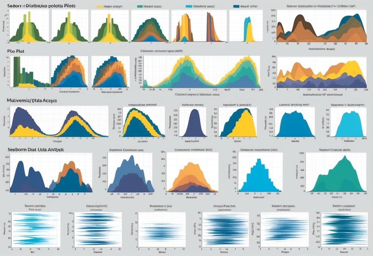
A colorful array of Seaborn distribution plots showcasing various plot types and multivariate data analysis

Multivariate data involves observations with more than one variable. Analyzing these data points is essential for identifying patterns and relationships among variables. Tools like Seaborn provide versatile plots that reveal these complex structures.

Visualizing Multi-dimension Data

Visualizing multivariate data involves showing relationships between multiple variables. Pairplot is a powerful tool, offering comprehensive visuals by creating a grid of scatter plots for continuous variables. It helps identify clusters, trends, and correlations.

Another useful tool is FacetGrid, which lets users plot subsets of data across multiple facets. This is helpful to compare different categories of a categorical variable while analyzing continuous characteristics.

Seaborn’s scatter plots can also visualize multivariate data by using color to encode a third variable’s information. These methods are crucial in exploratory data analysis to understand and interpret complex datasets better. Learn more about these techniques by exploring the detailed guide on multivariate data analysis.

Frequently Asked Questions

A person studying a chart of different distribution plot types for Seaborn

Seaborn offers a variety of options for visualizing data distribution in Python. In this section, users will discover how to work with distribution plots and learn about specific plotting functions and customization techniques available in Seaborn.

How can one create and interpret a seaborn distribution plot in Python?

To create a distribution plot in Seaborn, use the distplot or displot function. These plots help visualize the distribution of a dataset, providing insights into patterns such as central tendency and variability. Interpreting these plots involves examining features like peak areas, spread, and any skewness present in the data.

What are the key differences between histogram and distribution plots in seaborn?

Histograms are used to group continuous variables into bins, showing the frequency of occurrences in each bin. Distribution plots, on the other hand, can include kernel density estimation (KDE) which smoothens the appearance, providing a more detailed view of the data’s distribution shape.

Which seaborn function is used to visualize data distribution?

Seaborn features several functions for visualizing data distribution, such as distplot, displot, and kdeplot. These functions offer flexibility in how data distributions are displayed, including options for histograms, KDE, and empirical cumulative distribution functions (ECDF).

In seaborn, which plots are most suitable for visualizing statistical distributions?

For visualizing statistical distributions, Seaborn’s KDE plots, histograms, and pair plots are quite effective. Each offers unique ways to understand data spread and relationships. KDE plots are particularly helpful for seeing smooth distribution curves, while pair plots can examine multi-variate relationships.

Can you outline the steps to customize the appearance of seaborn distribution plots?

Customization in Seaborn is straightforward. By altering parameters like color, alpha, and bins, users can tailor plot aesthetics. Additionally, using matplotlib settings, plots can be further refined with customized axes, titles, and labels for improved clarity and presentation.

What are the various options for plotting bivariate distributions using seaborn?

Seaborn offers several options for bivariate distributions, including scatterplot, kdeplot, and jointplot functions.

These plots help visualize relationships between two variables, showing patterns like correlation and clustering.

Joint plots, for instance, combine scatter plots with histograms or KDE for enhanced insights.

Categories
Uncategorized

Learning Pandas for Data Science – Data Workflow Essentials Explained

Getting Started with Pandas

Beginning with Pandas involves setting up your Python environment and understanding key principles of this popular data analysis library.

This section will guide you through the installation process and introduce you to the foundational concepts critical for effective data manipulation and analysis.

Installation and Setup

To start using Pandas, one must first install Python if it is not already on the system.

Python can be downloaded from the official Python website. After installing Python, open a terminal or command prompt.

To install Pandas, use the following command:

pip install pandas

This will download and set up the Pandas library on your machine.

It’s also recommended to install Jupyter Notebook, an interactive tool that makes it easy to work with Python and Pandas. Use this command:

pip install jupyter

Once installed, launch Jupyter with:

jupyter notebook

This opens a notebook interface in the web browser, where you can write and execute Python code.

Having Pandas and Jupyter set up allows users to start exploring data science projects right away.

Pandas Fundamentals

Pandas is a powerful Python library for data management and analysis. The core components of Pandas are DataFrames and Series.

A DataFrame is a 2-dimensional labeled data structure, akin to a table in a database or Excel spreadsheet. A Series is a one-dimensional labeled array, like a column in a table.

To create a DataFrame, use:

import pandas as pd

data = {'Name': ['Alice', 'Bob'], 'Age': [25, 30]}
df = pd.DataFrame(data)

This snippet creates a simple DataFrame with names and ages.

Users can perform tasks such as filtering, grouping, and merging data. Mastery of these basics is essential for efficient data analysis and visualization using Pandas.

The library supports data cleaning, mutation, and aggregation, making it a favorite for those working with datasets in Python.

Understanding Data Structures

A laptop displaying a Pandas data workflow with charts and graphs, surrounded by books on data science and data structures

Data structures are fundamental in handling data with pandas. They help organize and manage data in a way that makes analysis straightforward and efficient.

Key structures include Series, DataFrames, and ndarrays.

Series and DataFrames

A Series is a one-dimensional array in pandas that holds data of a similar type. It’s similar to a list or array but with labeled indices. Labels make data retrieval more intuitive. For example, accessing data by label rather than by index number can simplify operations in various datasets.

A DataFrame is a two-dimensional, size-mutable, and heterogeneous tabular data structure. It consists of rows and columns, similar to a table in a database or a spreadsheet. DataFrames can hold different types of data across columns and are central to data manipulation in pandas.

Basic operations such as accessing, filtering, and summarizing data are streamlined with Series and DataFrames. They both allow for data alignment, handling of missing data, and integration with other libraries.

Working with Ndarrays

Ndarrays come from the NumPy library and represent N-dimensional data. They form the backbone for many operations in pandas.

While pandas adapts ndarrays into its Series and DataFrames, ndarrays themselves are ideal for numerical operations due to their performance efficiency.

These arrays are versatile, supporting various data types and operations like slicing, indexing, and mathematical transformations. Though not labeled like pandas structures, their speed and efficiency in handling large datasets make them useful in performing heavy computations before manipulating data in pandas.

Pandas smoothly integrates with these arrays, enabling the conversion of ndarrays into DataFrames with ease, enhancing data analysis capabilities by combining flexibility with efficiency.

DataFrames vs Series

While both Series and DataFrames are crucial in pandas, they suit different needs.

A Series is optimal for handling a single list of data, focusing on indexing and selection with labeled data. It is particularly useful when dealing with a single column or row from a DataFrame.

DataFrames, being two-dimensional, excel at handling structured tabular data, where rows and columns can vary in data types. This versatility supports complex data operations, including merging, joining, and reshaping.

The choice between using a DataFrame or Series depends on the dataset’s complexity and structure, with DataFrames providing more flexibility for detailed analysis of complex datasets.

Data Import/Export

A laptop displaying a pandas dataframe with columns and rows, surrounded by charts and graphs. A person's hand hovers over the keyboard, ready to input or export data

Data import and export are key tasks in data science for moving data into and out of software like Pandas. This process involves reading data from various file formats and saving manipulated data back into files. Understanding these tasks is crucial for handling data efficiently.

Reading CSV/Excel/SQL/JSON

Pandas provides several functions to read data from different formats.

The read_csv function is commonly used for importing data from CSV files. With a single line of code, one can load a CSV file into a DataFrame, making it easy to start analyzing data.

For Excel files, Pandas offers read_excel, which supports reading multiple sheet formats. This can be especially handy for datasets with various segments on separate sheets.

Data from SQL databases can be imported using SQL queries. The function read_sql allows users to read from SQL databases directly into Pandas, facilitating smooth data analysis without needing to manually export queries.

Similarly, JSON data can be loaded using the read_json function, which is helpful for web-based data or APIs that return JSON objects.

Exporting Data to CSV/JSON

Exporting data is as straightforward as importing it.

The to_csv function enables users to save DataFrames back into CSV format. Options include specifying the delimiter, handling headers, and more, giving flexibility in the export process.

For JSON files, to_json allows conversion of DataFrames into JSON format. This is popular for sharing data across web applications. JSON files are lightweight, making them ideal for long-term storage or data transmission on the web.

These functions ensure data remains accessible and shareable after processing, making it easier for further analysis or reporting.

Data Cleaning Techniques

A laptop displaying a Jupyter notebook with code for data cleaning using Pandas, surrounded by open textbooks and a notebook with handwritten notes

Data cleaning is a vital process in any data science workflow. It ensures that data is accurate, consistent, and free from errors. Key techniques include handling missing values, transforming data, and filtering rows and columns to prepare datasets for analysis.

Handling Missing Values

Missing values can negatively affect data analysis. You must first identify missing data, which can appear as blanks, “NaN” in Pandas, or “null” values.

Filling these gaps is crucial, and one method is using the Pandas fillna() function to replace missing data with specific values, such as the mean or median.

Dropping rows or columns containing numerous missing values is sometimes necessary. This can be done using dropna(). It’s important to consider the impact of these actions on the dataset’s integrity.

Another approach is to use interpolation, which estimates missing values based on available data points.

Data Transformation

Data transformation includes modifying data to improve its format or structure, which enhances analysis.

One such transformation is scaling, which adjusts data ranges. This is often done through normalization or standardization. The Pandas library offers functions like apply() and map() to help transform data efficiently.

You can also use log transformation to manage skewness in data distributions.

Converting categorical variables into numerical values using techniques like one-hot encoding is also essential.

Python libraries such as Pandas and SciKit-learn provide these capabilities, enabling data scientists to transform data effectively.

Filtering Rows and Columns

Filtering is essential for focusing analysis on relevant data segments. Boolean indexing is a powerful tool for this purpose.

It allows you to select data based on conditions, such as filtering rows where a column value exceeds a threshold. In Pandas, this can be achieved using expressions like df[df['column'] > value].

Column filtering involves selecting necessary features and discarding irrelevant ones, which helps reduce noise in the data.

Methods like loc[] and iloc[] in Pandas provide flexible ways to filter both rows and columns. Applying filters can significantly enhance data quality and analysis outcomes without altering the core dataset.

Data Manipulation and Transformation

Data manipulation and transformation are key processes in data science, often involving techniques like aggregating data, creating pivot tables, and performing vectorized operations. These methods help in refining raw data into a structured format that is easier to analyze and visualize.

Aggregating Data

Aggregating data is vital for summarizing information. By using functions like sum(), mean(), and count(), analysts can condense extensive datasets into meaningful summaries. This process helps in understanding trends and making data manageable.

For instance, calculating the average sales per quarter offers insights into business performance.

In Pandas, aggregation functions are applied to dataframes or series, allowing you to specify either rows or columns for the calculation. Such flexibility enhances the ability to generate custom insights.

An example might be calculating the total revenue for different regions using Pandas. This supports decisions by making trends more visible.

Pivot Tables and GroupBy

Pivot tables and the groupby function are essential tools for reorganizing data.

Pivot tables, similar to those in spreadsheet software, allow data to be summarized, compared, and analyzed across different dimensions. This is extremely helpful for identifying patterns.

The groupby function in Pandas is versatile, grouping data based on one or more columns. It enables detailed analysis by allowing operations like summation, averaging, and counting within each group.

For example, sales data can be grouped by product category to determine which category contributes most to revenue, enhancing understanding of market dynamics.

Vectorized Operations

Vectorized operations enhance performance by applying computations directly to array or table structures rather than iterating through elements. This approach is efficient for large datasets as it leverages low-level optimizations. The result is faster processing speeds and reduced complexity.

In Pandas, vectorization allows operations like element-wise addition, subtraction, or logical operations on dataframes.

Such operations are crucial for data transformation, enabling swift handling of datasets without explicit loops. For instance, calculating price increases across a large dataset can be achieved in a single step, allowing quicker insights into price trends.

Exploratory Data Analysis (EDA)

Exploratory Data Analysis (EDA) is a crucial step in data science. It helps data scientists and business analysts uncover patterns, spot anomalies, and test assumptions. This process involves various techniques, focusing on summary statistics and correlation analysis to draw meaningful conclusions from data.

Summary Statistics

Summary statistics provide a quick overview of data through key figures. These include mean, median, mode, standard deviation, and range.

By calculating these metrics, data professionals can get a sense of the central tendency and variability in the dataset. For instance, the mean shows the average value, while the standard deviation indicates how much data varies from the mean.

These statistics are essential in identifying outliers or unusual data points that might skew the results.

Using tools like Pandas in Python, such calculations are straightforward. Data scientists often rely on summary statistics as a foundational step in EDA, allowing them to make informed decisions about data preprocessing and analysis. This aids in ensuring data quality and reliability before diving into complex modeling.

Correlation and Statistical Analysis

Correlation and statistical analysis focus on relationships between variables.

Understanding these connections can highlight how one variable may predict or affect another.

Correlation coefficients, like Pearson’s or Spearman’s, measure the strength and direction of these relationships. A correlation near +1 or -1 indicates a strong relationship, while a value close to 0 suggests no correlation.

Statistical analysis goes beyond correlation by testing hypotheses or assessing the significance of relationships.

Techniques such as regression analysis help in predicting outcomes and understanding complex interactions within data.

These analyses are crucial for data scientists and business analysts to inform strategic decisions and guide further exploration. Leveraging Python libraries like SciPy and Matplotlib simplifies integrating these analyses within the data workflow.

Data Visualization

Data visualization is a crucial part of analyzing data with Pandas.

Tools like Matplotlib and Seaborn help create various visual representations.

These tools can be used for plotting different types of graphs, including bar plots and histograms, which are essential for understanding data distributions and trends.

Plotting with Matplotlib and Seaborn

Matplotlib is a popular library used for plotting graphs in Python.

It provides a wide range of plotting options from simple line graphs to complex 3D plots.

It’s known for its flexibility and comprehensive customization options.

Users can adjust everything from colors and line styles to axis labels and gridlines, making it a versatile tool for detailed visualization work.

Seaborn is built on top of Matplotlib, offering a higher-level interface for creating visually appealing and informative statistical graphics.

It simplifies tasks like drawing attractive plots in a few lines of code.

Seaborn includes built-in themes and color palettes, which make it easier to create professional-looking visualizations without extensive configuration.

Features like multi-plot grids and specialized plots for categorical data add depth to visualization capabilities.

Creating Bar Plots, Histograms, and More

Bar plots are essential for comparing categorical data.

They represent data with rectangular bars, the lengths of which are proportional to the values they represent.

Bar plots can be created efficiently using both Matplotlib and Seaborn, with customization options for colors, orientation, and grouped or stacked bars.

Histograms are crucial for visualizing the distribution of numerical data.

They display data using bins to show frequency counts of data intervals.

These plots help in understanding data spread and identifying patterns like skewness or the presence of outliers.

Both Matplotlib and Seaborn offer functions to create detailed histograms, making them invaluable for statistical analysis and initial data exploration.

Machine Learning with Pandas

Machine learning with Pandas involves preparing data, selecting features, and performing various analyses like regression.

This process often uses tools like scikit-learn for efficient data handling and model building.

Feature Selection

Feature selection is a vital part of using Pandas for machine learning.

It involves selecting the most relevant data features for a model. This step improves accuracy and reduces computation time.

Pandas can be used to manage and preprocess data, making it easier to identify important variables.

Using Pandas in combination with scikit-learn, users can automate feature selection with methods like recursive feature elimination or by applying feature importance scores.

These methods help in narrowing down the dataset to include only the features that significantly contribute to the model’s predictions.

Regression Analysis

Regression analysis with Pandas helps in understanding relationships between variables.

It is widely used to make predictions and model trends within datasets.

Tools like scikit-learn provide functions for different regression models, from simple linear regression to more complex methods.

Data must be clean and well-prepared in Pandas before applying regression models.

Pandas facilitates data processing by providing functions for handling missing data, normalizing values, and structured data formatting.

Effective data visualization can also be a part of this analysis, allowing users to visually interpret model outputs and assess the fit of regression lines.

This integration of Pandas and scikit-learn enables efficient workflows for predictive modeling.

Time-Series Analysis

Time-series analysis involves studying datasets where observations are recorded at specific time intervals.

It is essential for spotting trends, seasonal patterns, and cyclical changes, making it crucial in fields like finance, economics, and environmental studies.

Working with Time Series Data

Time series data is characterized by its time-ordered nature. Analysts often start by cleaning and preparing datasets to handle missing values and outliers. This preparation ensures the reliability of the analysis.

A common technique in time-series analysis is decomposition, which separates data into trend, seasonal, and residual components. This helps in understanding underlying patterns.

Forecasting future values based on historical data is an essential task in this context.

Utilizing libraries like Pandas can streamline processes such as data manipulation and visualization, which are key for effective analysis.

Resources like the Time Series Analysis with Python Cookbook offer practical recipes for handling such data efficiently.

Advanced Topics in Pandas

A laptop displaying a Pandas data workflow with charts and graphs on the screen. A notebook and pen sit beside it

When working with large datasets, it’s crucial to focus on performance tuning and memory optimization in Pandas. These practices improve task efficiency and reduce resource consumption, which is essential for handling big data effectively.

Performance Tuning

Optimizing performance in Pandas can be achieved through various methods.

One key approach is vectorization, which involves using Pandas functions that operate on entire arrays instead of iterating through elements. This makes operations significantly faster.

For example, using apply() can be slower compared to vectorized operations like mean() or sum().

Another method is using Cython or Numba for speeding up complex Python functions. This involves translating Python code to C for faster execution.

Additionally, choosing efficient data types for columns, such as category for string data that takes on a limited number of unique values, can enhance performance by reducing both processing time and memory usage.

Memory Optimization

Memory optimization ensures that processes run smoothly, even with limited resources.

One important strategy is to reduce memory usage by downcasting numeric types. For instance, converting float64 to float32 where precision is not critical can cut memory usage significantly.

Using chunksize in read functions helps manage memory by processing data in smaller portions. This is especially useful for reading large files without loading everything into memory at once.

Pandas also offers tools to parse only necessary data. For example, specifying columns while loading a dataset with usecols minimizes memory consumption by excluding irrelevant data.

Furthermore, converting data to more efficient formats, like storing DataFrames in Parquet files, can improve both memory usage and performance when dealing with big data and even when data is stored in HTML formats.

Applying Pandas in Real-world Projects

Using Pandas in real-world projects helps data scientists turn raw data into valuable insights.

Guided projects allow learners to apply skills practically on datasets like the Ebay Car Sales Data, showcasing how data analysis is executed in authentic scenarios.

Guided Project: Ebay Car Sales Data

In the Ebay Car Sales Data project, participants learn key data science skills by working with a dataset of used cars. This guided project provides a practical experience in cleaning, manipulating, and analyzing data using Pandas.

Learners focus on transforming messy data into clean, structured formats. This involves handling missing values, creating new variables, and extracting insights using various Pandas functionalities.

Such hands-on exercises are crucial for developing a strong understanding of data workflows, making it easier to tackle similar tasks in professional settings.

Case Studies and Scenarios

Real-world case studies often highlight how Pandas can streamline data workflows.

These scenarios show practical applications, such as using Pandas to analyze market trends, optimize operations, or improve decision-making processes.

Data scientists benefit from these experiences by understanding the significance of efficient data handling and processing. They learn how to create meaningful data visualizations and reports, which are essential for communicating findings and influencing business strategies.

Such projects help bridge the gap between theoretical knowledge and practical application.

They empower individuals to become proficient in data-driven decision-making, a critical skill in modern data science environments. By engaging with these examples, learners gain a clearer perspective on the role of data manipulation and analysis in everyday tasks.

Frequently Asked Questions

A laptop with a pandas logo open to a FAQ page, surrounded by data charts and graphs

This section covers key aspects of using Pandas for data science. It includes data manipulation, starting with data analysis, performing common cleaning tasks, handling missing values, managing datasets, and visualizing data.

What are the essential features of Pandas for data manipulation in data science?

Pandas offers data structures like Series and DataFrame that make data manipulation easy and efficient.

It allows filtering, sorting, and grouping data effortlessly. Functions like loc, iloc, and groupby are crucial for slicing data and analyzing it based on different criteria.

How can one start with data analysis using the Pandas library?

To begin data analysis with Pandas, one should first install the library using pip install pandas.

After installation, importing Pandas in a Python script is essential.

Using functions like read_csv or read_excel, data can be imported into a DataFrame for exploration and manipulation.

What are some common data cleaning tasks in Pandas and how are they performed?

Common data cleaning tasks include removing duplicates, renaming columns, and converting data types.

Pandas provides functions like drop_duplicates for duplicate removal and rename for renaming columns.

Converting data types can be done using astype.

How do you handle missing values in a dataset with Pandas?

Handling missing values involves identifying and dealing with them using Pandas methods.

The isnull function helps detect missing values, while fillna allows filling them with specific values or methods like forward fill.

The dropna function is used to remove any rows or columns with missing data.

Can you explain how to merge and concatenate different datasets using Pandas?

Pandas enables dataset merging using merge for joining DataFrames based on keys, similar to SQL joins.

Concatenation is achieved with concat, which combines DataFrames either vertically or horizontally.

These methods are vital for assembling large datasets from various sources.

What is the best way to visualize data directly from a Pandas DataFrame?

Visualizing data from a Pandas DataFrame can be easily done using the library’s integration with Matplotlib.

The plot function in Pandas generates basic plots like line graphs or histograms directly from a DataFrame.

For more advanced visualizations, using Pandas with libraries like Seaborn is effective.

Categories
Uncategorized

Learning about Pandas Applying Methods on Single and Multiple Columns: A Comprehensive Guide

Understanding Pandas and Dataframes

Pandas is a powerful library essential for data manipulation and analysis in data science. It provides robust data structures that simplify the process of handling data.

One of the primary structures in Pandas is the DataFrame. A DataFrame is similar to a table in a database or a spreadsheet. It contains rows and columns, making it easy to store and manage large datasets.

Pandas offers another data structure known as a Series, which is a one-dimensional array-like object. Each Series has an index that labels each element, allowing for easy access and manipulation.

A typical pandas DataFrame contains multiple Series, with each Series representing a column. Each column can hold different types of data, such as integers, floats, or strings.

Working with columns in a DataFrame is straightforward. You can easily add, remove, and modify columns to suit the analysis needs. The index, which labels the rows, assists with efficient data retrieval.

By using Pandas, analysts can easily perform operations such as filtering data, applying functions, and aggregating data. These capabilities make it an indispensable tool in data science workflows.

Pandas’ strength lies in its ability to handle large amounts of data efficiently. Whether working with simple datasets or complex, multi-dimensional data, Pandas provides the necessary tools and methods to streamline data operations.

Basics of Applying Functions to Dataframes

Applying functions to DataFrames can significantly improve data analysis efficiency. By using tools like the apply() method and lambdas, one can perform complex operations across entire datasets with ease. Understanding these tools is essential for effective data manipulation in Python using Pandas.

The Apply Method

The apply() method in Pandas is a powerful function that enables users to apply custom operations across DataFrame rows or columns. This method transforms data by introducing a specific function to each element within a designated axis.

For instance, applying a mathematical operation such as squaring all values in a DataFrame column is simplified using this method.

The syntax of apply() involves specifying the function and axis. By default, apply() uses the axis of columns. Users can determine how the function affects their data, making it versatile for various tasks.

For instance, summing values across rows or obtaining their mean can be streamlined efficiently. According to GeeksforGeeks, the apply() method empowers users to modify DataFrames creatively and effectively.

Using Lambdas with Apply

Lambdas are anonymous functions that offer a concise syntax for simple operations. Integrating lambdas with the apply() method enhances flexibility and simplifies code, especially when defining one-off operations.

These functions are commonly used within the apply() method to perform immediate transformations.

For example, using a lambda function to increment each DataFrame value by one involves minimal code. The lambda syntax is simple: df['column'].apply(lambda x: x + 1).

According to a tutorial by Dataquest, combining lambdas with apply() enables efficient vectorized operations without the need for traditional loops. This approach not only saves time but also ensures that the codebase remains clean and understandable.

Advanced Single Column Manipulations

Single column manipulations in Pandas are crucial for efficient data analysis. This section explores advanced techniques for handling single columns using Series objects and the map method. These techniques enhance data manipulation capabilities, enabling users to perform sophisticated operations with ease.

Series Object Operations

The Pandas Series object allows for powerful operations on a single column. Each column in a DataFrame can be treated as a Series, which means it can utilize the various methods specific to Series objects.

By using attributes like .str, which acts as an accessor, users can perform string operations directly on elements of a Series.

For numeric operations, functions like sum(), mean(), and apply() can be utilized. The apply() function is often used for custom operations on series elements, though there are performance considerations.

According to discussions on Stack Overflow, directly calling optimized Pandas methods is usually faster than applying custom functions using apply().

The Map Method

The map() method is a concise and efficient way to transform data in a single column, especially for simple value mappings. Often used on a Pandas Series, map() replaces or transforms each element according to a function or dictionary.

This method shines in tasks like replacing values or applying a transformation function.

For instance, using map() can replace categorical values with numeric codes efficiently. Datagy points out that while both apply() and map() can be used for data transformations, map() is specifically tailored to handling Series objects. It is especially beneficial when simple transformations are needed, ensuring efficient data manipulation.

Transforming Multiple Columns

Transforming multiple columns in a Pandas DataFrame can be efficiently accomplished using the apply function. It allows for complex operations across columns. Additionally, understanding how to aggregate data across columns is crucial for data analysis, especially when summarizing or combining results.

The Apply Function for Multiple Columns

The Pandas apply function is a powerful tool when working with multiple columns. By using it with an axis parameter, users can apply a function to rows (axis=1) or columns (axis=0).

This function is ideal for performing operations that need to account for multiple elements at once. For instance, combining two columns into a new one by summing their values or applying a custom transformation is straightforward.

When applying functions to multiple columns, it is common to define a function that takes a DataFrame row, performs the computation, and returns the desired outcome. The result is often returned as a Pandas Series, which integrates seamlessly back into the original DataFrame, facilitating further transformations or analyses.

Aggregate Data Across Columns

Aggregating data across columns involves combining data from two or more columns to form a single output. It is frequently used in data analysis to summarize results or generate new metrics from existing data.

Pandas offers several methods for aggregation, which can include simple functions like sum, mean, or custom aggregation functions. By specifying axis=1 within the apply function, users can efficiently aggregate across columns rather than down rows.

This method is particularly useful in scenarios like calculating the total score from individual subject scores or generating a composite index. It allows for exploration of relationships and patterns by transforming detailed data into summarized insights, invaluable in decision-making processes.

Enhancing Performance with Apply and Map

A computer screen displaying code for applying and mapping methods on single and multiple columns using Pandas

In data analysis with Pandas, performance is key. The apply() and map() methods offer ways to enhance efficiency. They are often used when built-in operations are not available for specific tasks.

For single column transformations, map() is ideal and is used directly on Pandas Series.

For more complex operations, apply() can be used. It works with both Series and DataFrames, making it highly versatile. You can pass custom functions to apply() for greater flexibility and control over the data.

While map() is limited to Series, apply() can handle both Series and DataFrame operations. This means it’s useful for operations spanning multiple columns, such as aggregating data or applying diverse transformations simultaneously.

When working with DataFrames, understanding when to choose between apply() and other methods can greatly impact performance. As noted in the article on Transforming Pandas Columns, it’s crucial to balance the use of these methods against more efficient, vectorized operations.

Both map() and apply() contribute extensively to the efficiency of data processing tasks. They can be used with functions like lambdas, enhancing their power in many situations. Yet, be cautious, as these methods can be slower compared to vectorized operations.

For optimizing complex data manipulations, integrating these methods can be advantageous, but always weigh their performance impact, especially on large datasets. Use apply() for row and column applications to maximize potential while maintaining speed.

Custom Function Integration in Pandas

Pandas allows users to integrate custom functions into the data manipulation process, offering flexibility and precision. These functions can be applied using the apply() method, which is useful when standard functions do not meet specific needs.

Custom functions can enhance processing by applying transformations or calculations to DataFrame columns. Lambda functions offer a concise way to create on-the-fly functions for quick tasks. Users can input these functions directly through the apply() method to modify DataFrame columns or rows.

When using custom functions, it’s essential to understand the role of arguments and keyword arguments. These allow greater control over the function’s behavior, ensuring it operates as expected across varying data.

Example

Consider a DataFrame where you need to apply a function to adjust values:

def multiply_values(x, factor=2):
    return x * factor

df['new_column'] = df['original_column'].apply(multiply_values, args=(3,))

The above code shows how to use custom functions with args to specify additional parameters.

Using the raw parameter can influence how the function interacts with the data. Setting raw=True passes data as a NumPy array for potentially improved performance, while raw=False ensures values are passed as a Series.

By incorporating custom functions into Pandas workflows, users can achieve intricate data manipulations efficiently. This approach allows them to leverage both simplicity and power, tailoring operations to fit their unique data processing requirements.

Working with Numpy Inside Pandas

Pandas can be significantly enhanced by integrating with NumPy. NumPy provides powerful tools for advanced data manipulation, making it a perfect companion for Pandas’ capabilities.

Using NumPy with Pandas often involves vectorized operations, which boost performance. These operations allow computations on entire arrays rather than iterating element by element. This is not only faster but also simplifies the code.

When handling DataFrames, the apply() method is useful for applying functions along an axis. It can use NumPy functions, leading to efficient computation.

For instance, calculating complex statistics across DataFrame columns can be streamlined using this approach.

Here’s a simple example: imagine a DataFrame containing numerical data. Applying np.sqrt() to a column will return the square root of each element. This task, powered by the efficiency of NumPy, is both fast and clear.

Another benefit is NumPy’s array slicing capabilities, helping to manipulate data selection within Pandas’ DataFrames. You can select and operate on subsets of data without iterating through the whole dataset, saving time.

Managing large datasets often requires operations across multiple columns. Using NumPy’s functions with Pandas lets users perform operations like aggregation or transformation efficiently, ensuring smooth data analysis processes.

By combining NumPy with Pandas, users tap into a robust toolkit for data manipulation. This partnership enhances the ability to deal with complex datasets, providing clear and streamlined paths to insights. Written concisely, code leveraging this integration remains both powerful and readable.

The Power of List Comprehensions in Pandas

List comprehensions are a powerful tool in Python for making code concise and readable. When working with Pandas, they provide an efficient way to handle data manipulations within columns.

These comprehensions compress complex operations into a single line, which can enhance performance by reducing the need for explicit loops.

Consider a scenario: one wants to compute a new column based on existing data. Instead of writing multiple lines of loop code, list comprehensions can achieve this elegantly.

For example, if there is a DataFrame df, the operation could look like this:

df['new_column'] = [x * 2 for x in df['existing_column']]

This single line quickly applies a transformation to each item.

Performance and Efficiency

List comprehensions generally run faster than similar operations using apply() when dealing with simple functions. They leverage the efficiency of list iteration in Python, providing a speed advantage, especially on large datasets.

Here’s a basic side-by-side comparison:

Method Code Example Speed (Example Setting)
List Comp. [x*2 for x in df['col']] Faster
Apply Method df['col'].apply(lambda x: x*2) Slower

While .apply() is versatile, list comprehensions excel in straightforward operations, making them ideal for quick and efficient data transformations.

Controlling Operation Flow with Parameters

In pandas, applying methods to DataFrame columns can be customized through various parameters. These parameters help modify how functions are applied, affecting results and efficiency.

Understanding Apply Parameters

When using pandas’ apply() function, the parameters allow users to control the method’s behavior.

One crucial parameter is axis, which determines if the function should be applied across rows (axis=0) or columns (axis=1). This influences how data is processed, significantly impacting performance and output.

Another parameter to consider is result_type. It formats the output of the apply function, particularly useful when the function returns a list or a series. Choosing the correct result type can prevent errors and maintain the DataFrame’s structure.

Advanced users can use applymap() for element-wise operations and groupby functions for aggregating data across groups.

Positional vs Keyword Arguments

In programming, understanding positional arguments and keyword arguments helps control function calls better.

Positional arguments are passed to the function in the order they appear. This means their position directly affects how they are interpreted. It’s essential to ensure they are in the correct sequence to avoid bugs.

On the other hand, keyword arguments are defined by explicitly naming each argument. This approach enhances readability and flexibility, especially when a function supports a long list of arguments. It also allows users to change the order without affecting functionality, providing ease of use and preventing potential errors.

Using keyword arguments can enhance clarity when using complex pandas operations, leading to more maintainable code.

Dealing with Missing Data in Function Application

Handling missing data is crucial when applying functions to DataFrames in pandas. Effective methods ensure cleaner results and prevent errors when using tools like the apply() method or applymap().

Apply Methods and NaN Values

When dealing with missing data in pandas, understanding how numerical operations interact with NaN values is essential.

The apply() method can be used to operate on DataFrame columns or rows while taking into account any NaN values.

To fill or transform NaNs, developers often use functions like fillna() in their apply() functions. This ensures that mathematical operations don’t yield unwanted results due to NaNs. It’s important to remember that NaN is treated as a float and can affect operations if not handled properly.

The applymap() function is useful when applying functions element-wise on DataFrames. Though its use is less common for missing data, it remains valuable when each cell needs processing, including those with NaN. Since NaN is common, knowing how to manage it can improve data analysis and prevent incorrect outputs when using these functions. More methods can be found for handling missing data like using fillna().

Using Applymap for Element-Wise Operations

Applymap is a powerful function in Pandas used for element-wise operations. It acts on every single value of a DataFrame, unlike functions like apply() which operate on rows or columns. This makes it perfect for applying a function across all columns and rows in a DataFrame.

The function applymap() is exclusively available for DataFrames. When there is a need to transform every element in a DataFrame, applymap is the go-to method. For instance, converting all elements to strings can be done easily with the use of applymap(str).

A practical example: suppose there’s a DataFrame with numerical values, and the task is to format each number as a percentage. Using applymap(lambda x: f"{x:.2%}") would efficiently convert each number into the desired format.

One should remember that applymap does not work with pandas Series. It’s designed to operate on the 2D data structure of DataFrames. For Series, the map() function is more appropriate.

When dealing with larger DataFrames, applymap can be less efficient than more direct methods due to its element-wise nature. Yet, its straightforward approach makes it an excellent choice for comprehensive data transformations. To learn more about using applymap for performing element-wise operations, you can explore further resources.

Assigning Data with the Assign Method

A person using a computer to apply the assign method on single and multiple columns in Pandas

The assign() method in pandas is a powerful tool for adding new columns to a DataFrame. This method is used to either append new data or update existing columns with ease.

Adding new columns with assign() is straightforward. It allows developers to specify the column name and assign data using keyword arguments. For instance, df.assign(new_column=data) creates new_column populated with data.

Example Usage:

import pandas as pd

df = pd.DataFrame({'A': [1, 2], 'B': [3, 4]})
df = df.assign(C=lambda x: x.A + x.B)

This example adds a new column C by performing operations on existing columns A and B.

Multiple columns can be added simultaneously with assign(). It accepts multiple arguments, each creating a new column. This feature streamlines data manipulation tasks. Read more about assigning multiple new columns.

The assign() method ensures that changes do not affect the original DataFrame. Instead, it returns a new DataFrame with the updates. This behavior preserves data integrity during operations.

Frequently Asked Questions

A panda bear mascot surrounded by question marks, demonstrating methods on columns

Applying functions in Pandas can streamline data analysis. This section addresses common questions about using the apply function with columns in a DataFrame, applying functions with arguments, and more.

How do you use the apply function to multiple columns in Pandas and create a new column?

To create a new column by using the apply function across multiple columns, use a lambda function within apply(). Set axis=1 to indicate row-wise operation. For example, df['new_col'] = df.apply(lambda x: f(x['col1'], x['col2']), axis=1). This approach was suggested by Statology.

What is the process to apply a function with arguments to a single column in Pandas?

For a single column, use the apply method and pass the function directly. If additional arguments are needed, supply them with the args parameter. For example, df['new_col'] = df['col'].apply(function_name, args=(arg1, arg2)).

How can you apply a function to all columns in a Pandas DataFrame?

Use the applymap() function to apply a function to each element in the DataFrame individually. This is useful for element-wise operations. df.applymap(function_name) applies function_name across all cells.

In Pandas, how can you apply multiple functions at once to a DataFrame?

The agg() function lets you apply several functions simultaneously. It can be specified for individual columns or the whole DataFrame. For instance, df.agg(['sum', 'mean']) computes both the sum and mean for each column.

What method is used in Pandas to apply a lambda function and return multiple columns?

To return multiple columns using a lambda, use assign() in combination with apply(). For instance, df = df.assign(new_col = lambda x: function(x['col1'], x['col2'])). This can efficiently create multiple columns simultaneously.

How can you apply the same condition to multiple columns simultaneously in Pandas?

A common way is to use loc[] together with apply().

For example, apply a condition like df.loc[:, ['col1', 'col2']].apply(lambda x: condition, axis=1). This allows conditions to be set on multiple columns at once based on a single lambda function.

Categories
Uncategorized

Learning T-SQL – DML: UPDATE and DELETE Techniques Explained

Understanding DML: Definition and Importance

Data Manipulation Language (DML) is a vital component of SQL. It refers to the set of commands used to manage data in databases. These commands include INSERT, UPDATE, and DELETE, which allow users to modify data stored in tables.

Key DML Commands

  • INSERT: Adds new data into a table.
  • UPDATE: Alters existing data.
  • DELETE: Removes data from a table.

Each of these commands offers flexibility to ensure data is accurately reflected in the database.

DML operations are essential for maintaining data integrity and accuracy. They allow users to dynamically interact with data as requirements change. Unlike Data Definition Language (DDL) that deals with database schema, DML focuses on data manipulation.

In SQL, DML statements enable real-time data processing and analysis. This is crucial for applications that require frequent updates, such as inventory systems or customer management platforms.

An important aspect of SQL statements involving DML is their ability to be controlled through transactions. Transactions help maintain consistency by grouping multiple operations into a single, atomic action. This ensures data is not left in an incomplete state.

In contemporary database management, DML plays a significant role. It empowers users to effectively interact with their data, ensuring it remains relevant and up-to-date. Understanding how to use DML commands proficiently is a fundamental skill for anyone working with relational databases.

Setting up the Environment

Before diving into learning T-SQL with UPDATE and DELETE commands, it’s crucial to prepare the right environment. This involves installing SQL Server and creating a sample database for practice. These steps are essential for understanding database management and data manipulation.

Installing SQL Server

The first step is setting up SQL Server. Download the installer from the official Microsoft website, where you can find different editions such as Express or Developer, both suitable for learning.

Run the installer and choose Basic installation for simplicity. Follow the setup instructions. Choose default settings unless specific configurations are needed. Make sure to enable SQL Server Authentication for flexibility with future logins. A strong password for the sa account is recommended.

Once installed, SQL Server Management Studio (SSMS) should also be downloaded and installed. It’s a tool for managing SQL Server, executing queries, and organizing databases. With SSMS, you can connect to your server and begin setting up databases.

Creating a Sample Database

With SQL Server and SSMS ready, the next step is creating a sample database. Open SSMS and connect to your SQL Server instance. Right-click Databases in Object Explorer and select New Database.

Enter a name for your database and click OK. The database is created immediately. To practice T-SQL commands, create a table using this script:

CREATE TABLE Employees (
    EmployeeID INT PRIMARY KEY,
    Name NVARCHAR(50),
    Position NVARCHAR(50),
    Salary DECIMAL(10, 2)
);

This table allows practicing both UPDATE and DELETE operations effectively. As a database administrator or learner, working with this setup aids in mastering essential database tasks.

The Role of Transactions in DML

Transactions play a crucial role in managing data modifications within SQL databases. They ensure that operations like updates and deletions are processed reliably, maintaining data integrity and consistency. A clear grasp of how transactions work is essential for data engineers to effectively manage these processes.

Begin Transaction

A transaction begins with a Begin Transaction statement. This marks the start of a sequence of operations that should be treated as a single unit of work. In data management, this is important to ensure that any changes made during the transaction are isolated and do not interfere with other processes.

For example, when multiple updates or deletes are needed, a transaction ensures that all operations succeed before any changes are made permanent. If an error occurs during any part of the process, the transaction can be rolled back to prevent data inconsistencies. This provides flexibility and reliability, which is vital in environments where data accuracy is crucial.

Commit and Rollback

Commit and Rollback are key elements in managing transactions. A Commit operation finalizes the changes made during a transaction, making them permanent. Any data modifications become visible to other users and applications. It’s essential to use Commit when the desired changes are error-free and verified, ensuring that the database remains accurate.

On the other hand, Rollback is used to revert any changes made during the transaction. If an unexpected issue arises or the intended outcome isn’t achieved, Rollback will undo all operations. This helps maintain data consistency by allowing data engineers to correct mistakes without leaving incomplete or incorrect data in the system.

Crafting the UPDATE Statement

Crafting an effective UPDATE statement in T-SQL allows for precise data modification within SQL databases. It is essential to understand the syntax, the role of the WHERE clause, and handling updates involving multiple tables.

Syntax and Structure

The structure of an UPDATE statement is crucial for successfully modifying data. The basic syntax involves specifying the table to update and setting new values for one or more columns. For example:

UPDATE table_name
SET column1 = value1, column2 = value2

This syntax must be clear to avoid accidental changes. Using aliases can help make the UPDATE statement more readable. Ensure that column names and values are correctly aligned to avoid errors.

Using the WHERE Clause

The WHERE clause in an UPDATE statement is vital for targeting specific rows. Without it, every row in the table would be updated, which can lead to unintended changes.

For example:

UPDATE table_name
SET column1 = value1
WHERE condition

Choosing the correct condition for the WHERE clause is essential to ensure that only the intended data is modified. This often involves using operators like =, >, <, and LIKE to narrow down the selection.

Handling Multitable Updates

Updating data in multiple tables is more complex and often involves joins. When two or more tables need modification, a JOIN clause may be required within the UPDATE statement.

Example syntax might look like:

UPDATE a
SET a.column = b.value
FROM table1 a
JOIN table2 b ON a.id = b.id

Handling multitable updates requires a clear understanding of relationships between tables. Ensuring that the join conditions are accurate will prevent incorrect data modifications. Proper indexing on join columns can also enhance performance.

Executing UPDATE Operations

Executing an UPDATE operation in SQL is essential for modifying existing data. Understanding both single record updates and batch updates with transactions can help data engineers maintain accurate and efficient databases.

Updating Single Records

When updating a single record, using the primary key is crucial to ensure accuracy. The primary key uniquely identifies each record in a table, allowing precise updates. For example, in T-SQL, the syntax to update a single record looks like this:

UPDATE table_name
SET column1 = new_value1, column2 = new_value2
WHERE primary_key_column = key_value;

Remember to use the WHERE clause to target specific records. Without it, the update will apply to all records in the table. This method is fundamental for tasks where only one record’s data needs to be modified.

Batch Updates with Transactions

Batch updates involve modifying multiple records at once, often requiring more complex queries. Transactions play a vital role by grouping multiple UPDATE operations. This ensures that either all changes are applied, or none at all, preserving data integrity.

Here’s a basic structure of a transaction in T-SQL:

BEGIN TRANSACTION;
UPDATE table_name
SET column_name = new_value
WHERE condition;
COMMIT TRANSACTION;

Using transactions is particularly important when updates affect related data across different tables. By doing so, a data engineer can prevent partial updates, which could lead to inconsistencies. Understanding these concepts enhances the ability to perform efficient and reliable database operations.

DELETE Statement Fundamentals

The DELETE statement in T-SQL is vital for removing data from tables. Mastery of its basic syntax and understanding how to use the WHERE clause efficiently are essential skills for database management. These aspects ensure that only the intended data is modified or removed.

Basic Syntax

The DELETE statement is used to remove data from a table in T-SQL. Its basic structure involves specifying the table from which the records need removal. A typical DELETE statement looks like this:

DELETE FROM table_name;

Without a condition, this command removes all rows from the table. This feature is powerful but risky if used without constraints. It’s crucial to use DELETE with caution to avoid accidental data loss. By default, a DELETE operation frees the space held by the records.

Utilizing DELETE as part of the CRUD operations (Create, Read, Update, Delete) allows developers to effectively manage and change data within relational databases. Proper understanding of its syntax is necessary for clear and efficient database maintenance.

Implementing the WHERE Clause

The WHERE clause is a key part of the DELETE statement that adds precision. It allows users to specify which rows should be removed instead of deleting all data from the table. A DELETE operation with a WHERE clause looks like this:

DELETE FROM table_name WHERE condition;

The clause ensures that only rows meeting the specified condition are deleted. This prevents unintentional data removal and maintains database integrity.

Implementing the WHERE clause requires a clear understanding of the table’s structure. Knowing how to apply conditions effectively can optimize data management and improve performance by minimizing unnecessary data manipulation. Using indexing and checking execution plans can further enhance the DELETE operation’s efficiency.

Advance DELETE Techniques

Effective DELETE techniques in T-SQL, such as using joins or setting cascade delete rules, can enhance database performance and integrity. These methods help maintain organized data by ensuring that deletions are efficient and consistent.

Deleting Data Using Joins

In T-SQL, using joins for delete operations is a powerful technique. This method is beneficial when data in one table is closely linked to another through a primary key and foreign key relationship. By using a join, it is possible to delete data from multiple related tables in a single query.

Consider a scenario with a Sales and Customers table. To remove entries from Sales where customers meet a certain condition, one might use:

DELETE FROM Sales
FROM Sales
INNER JOIN Customers ON Sales.CustomerID = Customers.ID
WHERE Customers.Status = 'Inactive';

This approach allows efficient management of data by targeting specific records linked across tables.

Cascade Delete Rules

Cascade delete rules are used to automatically delete related data in other tables. When a record in the primary table is deleted, related rows in a dependent table are also removed. This is achieved by setting up cascade deletes in the database’s referential integrity constraints.

For example, when setting up a relationship between Orders and OrderDetails, a cascade delete ensures that when an Order is deleted, all associated OrderDetails entries are automatically removed. This can be set up using T-SQL or via the database’s graphical tools.

ALTER TABLE OrderDetails
ADD CONSTRAINT FK_Orders_OrderDetails
FOREIGN KEY (OrderID) REFERENCES Orders(ID)
ON DELETE CASCADE;

This configuration reduces the need for separate delete statements and helps maintain database integrity, preventing orphaned records and streamlining multi-table operations.

Data Retrieval and DML

Data retrieval and Data Manipulation Language (DML) are key components of interacting with databases in T-SQL. They involve the use of SELECT statements to retrieve data, and DML operations such as UPDATE and DELETE to manipulate data.

Understanding how these elements work together is essential for effective database management.

The Interplay with SELECT

SELECT statements in T-SQL are vital for retrieving data from tables. They allow users to specify which columns to display and filter rows based on given conditions.

Selecting data does not alter the database; it only queries information.

In practice, SELECT often works with DML. For example, retrieving rows before applying updates ensures accuracy and precision in data manipulation.

In DML operations like UPDATE, one may first use SELECT to identify which rows meet certain criteria. This two-step approach maintains data integrity and reduces errors in large datasets.

SELECT also aids in testing delete operations by displaying the target data before deletion, providing a safe check.

Using Joins in Data Manipulation

Joins are crucial when manipulating data across multiple tables. They combine rows from different tables based on a related column.

In T-SQL, using joins with DML enables unified updates or deletions on linked data. For instance, an INNER JOIN can match records in two tables, ensuring updates are consistent.

When a DELETE operation involves multiple tables, joins can specify related records to remove. This prevents orphaned data and maintains relational database integrity.

Properly using joins in DML helps control complex updates or deletions, making sure each action reflects the intended changes seamlessly across tables.

Specialized DML Operations

In T-SQL, specialized DML operations enhance data handling. Key concepts include using defaults and identity properties for data validity, and leveraging powerful commands like TRUNCATE and MERGE for efficient data management.

Working with DEFAULT and IDENTITY

Understanding how DEFAULT and IDENTITY work ensures consistent data entry.

The DEFAULT function is used to set a pre-defined value for a column when no value is specified. This can prevent errors and simplify data entry. For instance, a column for order date might automatically fill with the current date if left blank.

The IDENTITY property is useful for assigning unique numbers to a column, commonly used for primary keys. It automatically generates a unique value every time a new row is added.

This eliminates the need for manual entry of unique identifiers, reducing the risk of duplication and ensuring data integrity.

Using TRUNCATE, MERGE, and ALTER

The TRUNCATE command is a fast way to remove all data from a table, preserving its structure. Unlike DELETE, TRUNCATE cannot be rolled back and doesn’t fire triggers, making it more efficient for large record sets.

MERGE is a versatile statement that simplifies complex operations like keeping two tables in sync. It allows users to perform inserts, updates, and deletes in a single operation.

This is particularly useful for data warehousing and ETL processes, offering a streamlined approach to adjusting data based on certain conditions.

ALTER enables modifications to existing database objects. Common uses include changing column data types or adding new columns. Unlike data manipulation language commands, ALTER is part of the data definition language and focuses on altering the structure itself rather than the data within.

Insights for SQL Professionals

Professionals dealing with SQL, especially data engineers and database administrators, must understand crucial aspects of DML, including best practices and how to avoid common pitfalls. These insights are essential for ensuring efficient and error-free database operations.

Best Practices in DML

Data manipulation language (DML) involves operations like updating and deleting data within a database. It’s important to follow best practices to maintain data integrity and performance.

Developers and administrators should always test DML commands in a safe environment before applying them to live databases. Using transactions in SQL helps ensure that operations are completed successfully or rolled back entirely in case of an error, which is crucial for maintaining data consistency.

Furthermore, when performing mass updates or deletions, breaking down large queries into smaller batches can prevent system overloads. This approach also makes it easier to troubleshoot if errors occur during the execution.

Using indexes wisely can drastically improve the performance of DML operations. However, overly relying on them can lead to increased storage space usage and slower updates. Regularly reviewing the structure and usage of indexes is also recommended to maximize efficiency.

Common Pitfalls and How to Avoid Them

Common pitfalls in DML operations can lead to data inconsistencies and performance issues. One major pitfall is neglecting transaction management. Without transactions, partial updates during errors might corrupt data.

Data engineers should also beware of deleting records without a backup. It’s a good habit to create backups or ensure a rollback plan is in place before major deletions.

Another common mistake is not considering the impact of foreign key constraints. Ignoring these can lead to errors or unintentionally deleting linked data.

Incorporating cascade actions carefully and understanding table relationships can help prevent these issues.

Finally, poorly constructed queries can lead to slow performance. Developers should regularly analyze query plans and optimize their SQL code to avoid inefficiencies.

Keeping queries as simple and targeted as possible reduces the chance of hitting performance bottlenecks.

Security Concerns in DML Statements

Security is a critical aspect when handling DML statements like UPDATE and DELETE in T-SQL. Proper management can help prevent unauthorized access and data corruption.

DML Triggers are one tool to enhance security. They execute T-SQL code in response to data modifications, such as INSERT, UPDATE, or DELETE statements, to monitor and control activities.

Permissions play a key role in securing DML operations. Restrict access using Data Control Language (DCL) commands like GRANT and REVOKE. Only authorized users should have the ability to perform CRUD operations.

Monitoring is another important aspect. Keeping an eye on DML activities can help identify suspicious behavior.

Using logs and audits ensures that data changes are traceable and can be reviewed.

Additionally, consider implementing security measures such as encryption and role-based access control to safeguard sensitive information. These measures help protect data even if someone gains access to the system.

It is crucial to regularly update security settings and test systems for vulnerabilities to adapt to new threats. By actively managing the security of DML statements, database administrators can prevent data breaches and maintain system integrity.

Frequently Asked Questions

Learning T-SQL involves understanding how to use commands like UPDATE and DELETE effectively. Familiarity with the distinctions between DML and DDL commands is also important. Here are answers to some common questions about these topics.

How do I perform an UPDATE operation using T-SQL and what are the best practices?

An UPDATE operation in T-SQL is used to modify existing records in a table. To do this, use the UPDATE statement followed by the table name.

It is crucial to include a WHERE clause to specify which records should be updated. Without it, all records in the table may change by accident.

It’s best to back up data before running large updates.

What are the steps to correctly use the DELETE statement in T-SQL?

To use the DELETE statement, write DELETE FROM followed by the table name. Like with updates, a WHERE clause should specify the precise records to remove. If omitted, the command will delete all rows.

Checking foreign key relationships is essential to avoid integrity issues.

In SQL, what distinguishes DML commands from DDL commands?

DML, or Data Manipulation Language, includes commands like INSERT, UPDATE, and DELETE that modify the data within tables. DDL, or Data Definition Language, encompasses commands like CREATE, ALTER, and DROP, which define the structure of database objects. They serve different purposes, with DML focusing on data, while DDL deals with the framework.

Can you demonstrate how to use a SELECT statement within an UPDATE query in T-SQL?

A SELECT statement can be embedded within an UPDATE query to dynamically set the updated values. This is achieved using the SET clause with a subquery.

For example, UPDATE table_name SET column1 = (SELECT column2 FROM another_table WHERE condition) allows the update of column1 based on the value retrieved by the SELECT statement.

How do you ensure data integrity when performing DELETE operations in T-SQL?

To maintain data integrity during DELETE operations, enable referential integrity constraints like foreign key relationships. These constraints prevent the deletion of records that could cause orphaned records in related tables.

Always ensure backups are available before performing delete operations, especially in a production environment.

What are common mistakes to avoid when using UPDATE and DELETE commands in T-SQL?

Common mistakes include omitting the WHERE clause. This can lead to unintended changes or deletions across an entire table. Another mistake is not previewing changes with a SELECT query to confirm the right records are targeted. It’s also important to consider the impact on related data and maintain back-ups to recover from errors.

Categories
Uncategorized

Learning Data Analysts Roles: Essential Skills and Responsibilities

Understanding the Role of Data Analysts

Data analysts play a vital part in transforming raw data into meaningful insights. They focus on examining data trends and patterns through advanced techniques.

Responsible for providing data-driven decisions, data analysts work with various tools to visualize and present their findings. This helps organizations enhance their strategies and achieve better results.

Core Responsibilities

Data analysts are tasked with collecting, cleaning, and organizing data. These tasks ensure that data sets used for analysis are accurate and relevant.

They also conduct statistical analyses to uncover patterns or trends. Analyzing the data helps provide actionable insights which businesses can use to improve their strategies.

Further, data analysts create clear and effective data visualizations that allow stakeholders to easily understand complex data.

By turning data into visual stories, they help guide data-driven decisions. Data storytelling, using understandable language and visuals, is essential to effectively communicating findings.

Key Technical Skills

A data analyst should be well-versed in data analysis tools and techniques.

Key technical skills include proficiency in software like SQL, Excel, and specialized analytics programs. Data visualization tools like Tableau or Power BI are also crucial for developing rich visual representations.

Understanding programming languages such as Python or R aids in analyzing large data sets.

Analysts must possess strong problem-solving skills. Their ability to identify and resolve data inconsistencies plays a critical role in the accuracy of their analyses.

Technical skills are complemented by excellent communication skills to effectively share insights and recommendations with non-expert audiences.

Data Analyst vs. Data Scientist

Though data analysts and data scientists both work with data, their roles differ in focus and depth. A data analyst primarily examines data to find actionable information and patterns. The role includes data cleaning, organizing, and basic reporting. Their work often centers on descriptive and diagnostic data use.

In contrast, a data scientist delves more into predictive modeling and machine learning. They develop advanced algorithms that help forecast future trends based on historical data.

Data scientists tend to work with larger data sets and use more complex tools, making their technical expertise usually broader. Analysts and scientists thus represent different steps of the data-driven decision process within a business.

Essential Data Analysis Tools

In the world of data analysis, certain tools are fundamental for extracting, analyzing, and presenting information. These tools range from databases that store data to advanced software for in-depth analysis, ending with platforms that help in visualizing findings.

Relational Database Management

Relational databases are crucial for storing and managing large amounts of data. SQL (Structured Query Language) is a powerful language used to interact with these databases.

Many data analysts rely on SQL for tasks such as querying data, updating information, and maintaining data integrity.

In addition to SQL, platforms like Microsoft Excel are often used in conjunction with databases. Excel provides functionalities like PivotTables, which help in summarizing and analyzing data efficiently.

These tools enable analysts to manage and retrieve data quickly, which is essential for making informed decisions.

Advanced Analysis Software

For deeper data analysis, software like Python and big data technologies including Hadoop and Spark are indispensable.

Python is favored for its ease of use and extensive libraries that support statistical analysis and machine learning. Analysts use Python to automate data processing and perform complex calculations that are not feasible in other tools.

Hadoop and Spark are frameworks that manage large datasets across clusters of computers, making them ideal for handling big data.

These technologies allow analysts to process and analyze vast amounts of data efficiently, which is key in extracting insights from big data.

Visualization and Reporting Tools

Visualization is a vital component of data analysis, allowing analysts to present their findings clearly.

Tools like Tableau and Power BI are popular for creating visual representations of data. These platforms help transform raw data into interactive dashboards, charts, and reports, making complex data easily understandable.

Both Tableau and Power BI offer features that allow for real-time data updates and in-depth exploration of datasets.

These visualization tools are crucial for communicating insights effectively to stakeholders who may not be familiar with raw data analysis. Furthermore, Excel remains a staple tool for creating detailed reports and conducting basic data visualization.

Statistical Analysis and Data Modeling

A person analyzing data on a computer, surrounded by graphs and charts, with a data modeling software open on the screen

Statistical analysis and data modeling form the backbone of understanding data in depth. These processes help in discovering patterns, making predictions, and evaluating outcomes with accuracy. They facilitate actionable insights and predictive analytics crucial for business success.

Applying Statistical Methods

Statistical analysis is essential for extracting meaningful information from raw data. It involves techniques like regression analysis, hypothesis testing, and variance analysis to identify trends and relationships.

Data analysts use these methods to make sense of complex datasets, enabling informed decisions. In organizations, this kind of analysis is crucial for understanding customer behaviors, market trends, and operational efficiencies.

Analysts rely on tools like R and Python, which have rich libraries for statistical computations. These tools allow for robust statistical processes, reducing errors and increasing reliability, which is vital in sectors such as finance and healthcare.

Creating Predictive Models

Predictive models are the result of applying statistical methods to forecast future events. Data modeling involves designing mathematical models that predict outcomes based on historical data.

A key component is using machine learning algorithms to enhance model accuracy.

Through techniques like decision trees and neural networks, these models can predict customer demand, assess risks, or even personalize product recommendations.

Data analysts must focus on creating and validating these models to provide reliable predictions. This process involves iterative testing and feedback loops.

Understanding model limitations and continuously refining them is important for successful predictive analytics and maintaining trust in the insights derived.

Effective Data Communication

A data analyst presenting charts and graphs to a group of attentive colleagues in a modern conference room

Effective communication in data analytics involves both conveying complex data insights clearly and engagingly and working with stakeholders. Mastering these skills enables data analysts to present information in a way that drives decision-making and ensures successful collaboration.

Storytelling with Data

Data storytelling is a crucial skill that transforms raw data into a narrative that is easily understood. By using data visualization tools like Excel, Tableau, or Power BI, analysts can create charts and graphs that highlight trends and patterns.

This helps in simplifying complex information, making it more digestible.

The story often follows a structure, including an introduction, main content, and conclusion. This approach aids in engaging the audience and conveying the key insights effectively.

Through a well-crafted story, readers can better understand the implications of the data, which is essential for strategic decision-making.

Interacting with Stakeholders

For a data analyst, communicating effectively with stakeholders is vital. Stakeholders may include managers, team members, or clients who rely on accurate and meaningful insights.

Analysts need to adapt their communication style depending on the audience’s technical expertise.

Active listening and asking the right questions help to clarify stakeholder needs, ensuring the analysis addresses their concerns.

Additionally, involving stakeholders throughout the process enhances transparency and trust.

By presenting findings clearly using accessible language and relevant visuals, analysts can support stakeholders in translating data into actionable strategies.

These communication skills are essential for success and enable a data analyst to play a significant role in decision-making processes across various industries.

Data Cleaning and Preparation

A person organizing and sorting data into clean, structured format for analysis

To get the best results, data cleaning and preparation are essential for transforming raw data into a format ready for analysis. By utilizing various techniques, one can ensure that the datasets are accurate and dependable, creating a strong base for further examination.

Data Wrangling Techniques

Data wrangling refers to the process of converting raw data into a more usable form. This includes steps like removing duplicates, filling in missing values, and transforming data formats.

Tools such as Python and libraries like Pandas are often used to automate these tasks, saving time and minimizing errors.

Common techniques involve normalizing data and aggregating information from multiple sources. For instance, data analysts regularly use methods to handle outliers and irrelevant data points, ensuring the datasets are consistent.

Incorporating these practices enhances the quality and reliability of the data, which is crucial for any data analysis project.

Ensuring Data Quality

Maintaining high data quality is vital to the success of any analytical work. It involves validating data accuracy and checking for inconsistencies.

Data analysts must employ rigorous methods to ensure the data’s integrity, such as running regular audits and validation checks.

It’s important to have a systematic approach for correcting any errors found. This can include creating validation rules or using automated tools to flag anomalies.

Analysts often rely on data cleaning methods to scrutinize datasets, ensuring they meet the required standards before proceeding with analysis.

An organized data environment supports better decision-making and leads to more reliable insights.

Business Intelligence and Analytics

A group of analysts review and interpret data charts and graphs in a modern office setting

Business intelligence (BI) and analytics play crucial roles in supporting data-driven decisions within organizations. These processes help in turning raw data into meaningful insights, enabling business analysts and business intelligence analysts to identify trends and make informed choices.

Integrating BI in Data Analysis

Integrating BI into data analysis involves using tools and technologies to collect, store, and analyze data. This integration allows businesses to transform complex data sets into easy-to-understand formats.

BI tools, such as dashboards and reporting software, provide visuals like charts and graphs that simplify data interpretation for business analysts.

BI helps organizations in identifying operational efficiencies, spotting market trends, and recognizing customer preferences.

When business intelligence is effectively integrated, companies can ensure that their data analysis solutions support strategic goals, offering a competitive edge in the marketplace.

Advanced analytics techniques, including predictive modeling and machine learning, can enhance this integration by adding depth and accuracy to data-driven decisions.

Extracting Actionable Insights

Extracting actionable insights from data is a critical function of business intelligence. By analyzing data trends and patterns, business intelligence analysts can forecast outcomes and influence strategy.

This requires the ability to interpret data accurately and predict future scenarios, which is crucial for businesses looking to adapt and grow.

Tools and techniques such as data mining and cluster analysis enable the extraction of valuable insights that inform decision-making processes.

The result is a deeper understanding of business performance and customer behavior. This approach helps in optimizing marketing strategies, improving operational efficiencies, and enhancing customer satisfaction, all of which are essential for sustainable business success.

Specialized Areas of Analysis

A data analyst surrounded by various charts, graphs, and computer screens, analyzing specialized areas of data

Specialized areas of data analysis play a crucial role in various industries. With advancements in technology, data analysts are needed to address unique challenges across different sectors and emerging fields.

Sector-Specific Data Analysis

Data analysts often focus on particular industries, tailoring their skills to meet specific needs.

For instance, in healthcare, analysts work to manage and interpret patient data, aiding in clinical decisions and improving patient outcomes.

In finance, they assess market trends and financial risks, providing insights for better investment strategies.

In other areas like retail, data analysts focus on consumer behavior to optimize sales and marketing strategies. Information security analysts in sectors such as IT work to prevent data breaches by analyzing security breaches and developing protocols to strengthen the defenses.

Emerging Fields and Technologies

With technology evolving rapidly, new avenues in data analysis have emerged.

The field of machine learning and big data offers opportunities to develop models that predict trends and automate processes.

Analysts work with machine learning models to create advanced algorithms that improve decision-making and efficiency.

Data mining allows for deeper exploration of large datasets, uncovering patterns and correlations not immediately obvious.

As these technologies advance, new roles such as data engineers and statisticians are more crucial, focusing on creating architectures that support complex data systems and analytics.

These positions require specialized skills in statistics and programming, driving innovation across various sectors.

Career Path and Progression

A flowchart showing the progression of a data analyst's career path, with various roles and responsibilities branching out from entry-level to senior positions

The career path for a data analyst involves a range of opportunities for growth, educational advancement, and possible transitions to related fields. Individuals often start in junior roles and can move to senior positions as they gain experience. Education plays a crucial role in advancing one’s career. Transitioning to related roles like data scientist or operations analyst is also common.

From Junior to Senior Roles

As individuals begin their careers in data analysis, they often start as associate data analysts. In this role, they focus on collecting, processing, and performing statistical analyses on data.

With experience, they may progress to become mid-level analysts. At this stage, they work on complex projects and might lead small teams.

Continuing from mid-level, a professional may become a senior data analyst. In this position, responsibilities expand to include strategic initiatives and influencing decision-making processes. They also mentor junior staff.

Career advancement depends heavily on demonstrated skills and accomplishments, along with the ability to drive results in data-driven projects.

Academic and Continuous Learning

Education serves as a foundation for a career in data analysis. While a bachelor’s degree in fields such as statistics, computer science, or mathematics is often required, some may opt for a master’s degree to further enhance their skills.

Continuous learning is essential, as technology and methodologies in data analysis frequently evolve.

Many analysts participate in online courses, workshops, and seminars to stay current with industry trends. Certifications in specialized tools, like SQL or Python, can also improve career prospects.

This continuous dedication to learning helps analysts adapt to advancements in the field and enables them to take on more complex roles over time.

Transitioning to Related Roles

Data analysts often have opportunities to transition into different roles within or outside their organization. Many choose to become data scientists, which requires additional skills in machine learning and predictive modeling.

Others may pivot towards becoming operations analysts, focusing on improving business processes.

These transitions allow for broader career opportunities and can lead to roles that involve more strategic planning and decision-making.

Gaining expertise in data visualization and business intelligence tools can facilitate these transitions, providing the necessary skills to excel in these new capacities and enhance career advancement.

Industry Standards and Best Practices

A data analyst reviewing industry standards and best practices in a modern office setting with multiple computer screens and data visualizations

Data analysts navigate a world grounded in precise standards and ethical guidelines. Ensuring data accuracy and legal compliance forms the backbone of effective data management.

Maintaining Data Integrity

Data integrity is vital for reliable analysis. Data integrity means upholding accuracy and consistency over its lifecycle. Analysts prioritize collecting and organizing precise data to facilitate quality insights.

Techniques for maintaining integrity include using tools like R programming for data validation. Analysts often rely on robust data sources and implement systematic checks.

Maintaining data integrity is crucial when dealing with big data, where errors can significantly impact outcomes. Using backup plans and rigorous validation processes can help minimize risks.

Keeping data secure is another critical aspect, often involving collaboration with an information security analyst to protect against breaches. This ensures collected data remains unaltered and trusted.

Adhering to Legal and Ethical Guidelines

Data analysts must follow strict legal frameworks to protect privacy and ensure ethical use of information. Regulations like GDPR set clear rules about data handling and consent.

Compliance requires a firm grasp of legal standards and company policies. Analysts should receive regular training on privacy laws to stay updated. Understanding these frameworks helps prevent data misuse and maintains public trust.

They also follow ethical guidelines to avoid biases in data interpretation and presentation. Data literacy programs can enhance understanding of ethical considerations. Awareness fosters responsible data use and creates a transparent working environment.

Problem-Solving and Critical Thinking

A data analyst surrounded by charts, graphs, and a computer, analyzing and problem-solving to find patterns and insights

Effective problem-solving and critical thinking are crucial for data analysts. They involve evaluating complex datasets and drawing meaningful insights. These skills help analysts break down challenges and create data-driven solutions.

Approach to Tackling Data Challenges

Data analysts are often faced with complex tasks that require a strategic approach. They begin by clearly defining the problem. This first step is essential to ensure that efforts are focused and effective.

Once the problem is understood, they gather relevant data, ensuring its accuracy and completeness.

Next, they use powerful tools and techniques to clean and process the data. For example, data analysts might use SQL to sort and filter large datasets with ease.

Applying statistical methods is another common practice to analyze and interpret the information accurately.

The ability to spot patterns and anomalies in data is critical. Data analysts leverage skills like critical thinking and problem-solving to develop hypotheses and test them.

They iterate on their approach based on findings, refining their analyses to better understand the underlying data story.

Developing Analytical Thought Process

Analytical thinking is at the core of data analysis. It requires a logical and methodical approach, where questioning assumptions is key.

Analysts must examine all angles of a problem before drawing conclusions. They need to employ strategies that foster a deep exploration of data.

Building an analytical thought process involves training in varied analytical techniques. Data analysts enhance their skills by engaging in activities that demand logical reasoning and precision.

Working with diverse datasets helps them build a robust analytical mindset.

Moreover, analysts continuously seek knowledge to stay updated with the latest tools and techniques. This ongoing learning develops their ability to break down complex problems into manageable parts. Such expertise enables them to find correlations and causations within the data confidently.

Data Analysts in the Job Market

A group of people studying charts, graphs, and data sets to learn about the roles and responsibilities of data analysts in the job market

Data analysts are vital in today’s data-driven business environment, as they help companies make informed decisions. This section explores the high demand for these professionals and what they can expect to earn in this dynamic field.

Demand and Job Security

Data analysts are in high demand as businesses across industries look to leverage data for strategic insights. Companies depend on data analysts to identify patterns and trends that inform business decisions.

The increasing use of AI to handle routine data-related tasks allows data analysts to focus on critical analysis and strategy. This shift has further escalated the need for skilled analysts, making the profession both secure and promising.

Many large companies like Cigna offer diverse roles, including claims analysis and risk assessment, demonstrating the importance of data analysts in various sectors.

Those starting a career as a data analyst can expect a stable job market with numerous opportunities for advancement and specialization, especially as data continues to grow in importance in decision-making processes.

Understanding the Average Salary

The average salary for data analysts reflects their crucial role in business operations. Salaries vary depending on factors like location, experience, and industry.

Entry-level data analysts can expect competitive starting salaries, which often increase with experience and expertise in tools like Python and R. These programming languages are frequently sought in job postings, highlighting their importance in the data analyst toolkit.

Higher-level roles offer increased pay, with salaries indicating the growing recognition of data analysis as a valuable skill. This compensation is representative of the value placed on insights and strategies developed from data analysis.

Consistent demand and attractive salaries make data analyst careers appealing for those interested in data-driven problem solving.

Enhancing Skills with Training and Certifications

A person studying and completing various training and certification programs related to data analysis, surrounded by books, a computer, and educational materials

To excel in data analysis, it’s crucial to focus on education that targets both technical and coding skills. Training programs and certifications can guide learners to proficiency in these areas, providing validation and a competitive edge.

Identifying Beneficial Courses

When seeking the right data analyst courses, it’s important to look for those that cover essential technical skills. Courses on programming languages such as Python, R, and SQL are vital. These enable analysts to manipulate and interpret data effectively.

Online platforms like DataCamp and Google’s Data Analytics Certificate offer structured learning paths. These courses often provide a mix of lectures, hands-on projects, and assessments that help build confidence in coding and analytical abilities.

Selecting courses with real-world projects ensures practical application of learned skills.

Certifications to Validate Expertise

Certifications serve as evidence of a data analyst’s capabilities and expertise in the field. Popular certifications include the Microsoft Certified: Data Analyst Associate and the Google Data Analytics Professional Certificate.

These credentials can enhance job prospects by demonstrating knowledge and skills.

Microsoft Learn offers pathways to prepare for these exams, focusing on data visualization, modeling, and report design.

Certifications are not only useful for validating skills but also for keeping up-to-date with changing technologies. Targeting certifications that are recognized industry-wide adds credibility to a professional’s profile and can be a stepping stone for career advancement.

Frequently Asked Questions

Data analysts play a crucial role in interpreting data to help businesses make informed decisions. This section covers key aspects of the role, qualifications, and skills needed for a successful career in data analysis.

What are the primary responsibilities of a data analyst?

Data analysts collect, process, and analyze large datasets to identify trends and insights. They create reports and visualizations to communicate findings, helping guide business strategies and decisions.

What qualifications are necessary for a career in data analysis?

A bachelor’s degree in fields like mathematics, computer science, or statistics is typically required. Proficiency in tools such as Excel, SQL, and data visualization software is also important.

How can one become a data analyst without prior experience?

Entry into data analysis can be achieved through online courses and certifications. Platforms like Coursera offer relevant learning programs.

Building a portfolio with projects demonstrating skills can significantly help.

Which skills are essential to succeed as a data analyst?

Essential skills include proficiency in data analysis tools, strong statistical knowledge, and the ability to communicate complex findings clearly. Problem-solving and critical thinking are also vital.

What is the typical salary range for a data analyst?

The salary of a data analyst can vary based on experience, location, and industry. Entry-level positions generally start from $50,000 annually, while experienced professionals can earn significantly more.

What do entry-level data analyst positions typically entail?

Entry-level roles often involve data collection, cleaning, and basic analysis tasks. These positions are designed to help new analysts develop their problem-solving skills and technical proficiency.

Categories
Uncategorized

Learning about SQL Rollups: Simplifying Data Aggregation

Understanding SQL Rollup

SQL Rollup is a tool used in database queries to summarize data and calculate subtotals and grand totals efficiently. It allows for various levels of aggregation within a hierarchy, simplifying complex data into more digestible forms.

Defining Rollup

Rollup is an extension of the SQL GROUP BY clause. It simplifies data analysis by providing aggregate data across multiple dimensions.

For instance, when dealing with sales data for various products, Rollup can compute subtotals for each product category and a grand total for all sales.

This is beneficial in organizing and interpreting large datasets.

The syntax usually involves listing columns in a hierarchy, such as ROLLUP(A, B, C), where SQL processes the data by grouping and aggregating based on this order. This creates multiple grouping sets, which include all possible combinations of these columns, along with the overall total.

The Purpose of Rollup in SQL

Rollup serves the essential function of data aggregation. When a database contains hierarchical data, Rollup efficiently computes subtotals at each level of the hierarchy.

For example, in a sales report, it can generate totals for each region, then for each country within a region, and finally a grand total for all regions. This is particularly useful for reports that require data to be summed up at different levels.

The SQL ROLLUP also aids in generating these comprehensive reports by calculating necessary subtotals and the grand sum without manually writing multiple queries, thus saving time and reducing complexity.

SQL Rollup Syntax

The SQL Rollup provides a way to create summaries in query results by adding subtotals and grand totals. Understanding its syntax helps users create efficient data aggregations and can be particularly useful in reporting scenarios.

Basic Rollup Syntax

In SQL, the Rollup syntax is used within the GROUP BY clause. It allows the user to generate summary rows in the result set. The basic format is as follows:

SELECT column1, column2, aggregate_function(column3)
FROM table_name
GROUP BY ROLLUP (column1, column2);

When using Rollup, it processes columns inside the parentheses from left to right. This generates aggregate data, like subtotals, for each level of hierarchy in those columns. The final result includes these subtotal rows and a grand total row, if applicable.

Mastering this syntax enables analysts to quickly produce complex reports.

Rollup with Group By Clause

When using Rollup with a GROUP BY clause, the Rollup is an extension that simplifies creating multiple grouping sets. While a regular GROUP BY groups the data by each unique set, adding Rollup expands this by including additional subtotal rows for each level and a grand total.

The Rollup option does not produce all possible combinations of groupings like the CUBE function. Instead, it controls the hierarchical grouping, ensuring efficient computation.

In SQL Server, it’s important to note that Rollup uses existing columns and extends their groupings without changing the original order. This feature makes it a valuable tool for summarizing complex datasets efficiently in business environments.

Working with Aggregate Functions

In SQL, aggregate functions like SUM, COUNT, and AVG are powerful tools for summarizing large datasets. These functions, combined with ROLLUP, can generate important insights, such as subtotals and grand totals, to aid decision-making.

Using Sum with Rollup

The SUM function is essential for adding values in a dataset. When used with ROLLUP, it can provide both subtotals for groups and a grand total. This feature is useful for generating sales reports or financial summaries.

For instance, to calculate the total sales per product category and overall, the query might look like this:

SELECT category, SUM(sales)
FROM sales_data
GROUP BY ROLLUP(category);

In this example, each category’s total sales are calculated, and ROLLUP adds an extra row showing the total sales for all categories combined. This method simplifies understanding of both detailed and aggregate sales figures, making data evaluation more efficient.

Count, Avg, and Other Aggregates

Aggregate functions such as COUNT and AVG also benefit from using ROLLUP. The COUNT function is used to tally items in a dataset, while AVG calculates average values.

For example, using COUNT with ROLLUP helps analyze customer visits per store, then add a grand total of all visits:

SELECT store, COUNT(customer_id)
FROM visits
GROUP BY ROLLUP(store);

Similarly, AVG with ROLLUP provides average sales data per region, with an overall average row. These applications are invaluable in identifying trends and assessing performance across categories. By leveraging these functions with ROLLUP, SQL users can efficiently interpret various data points.

Hierarchical Data and Rollups

In SQL, the handling of hierarchical data often involves organizing data into different levels. This organization can make data analysis more structured and meaningful. Rollups play a crucial role in this process by simplifying the generation of summary rows for various levels within a hierarchy.

Understanding Hierarchical Aggregation

Hierarchical aggregation involves arranging data into a parent-child structure. This is common in business settings where information is segmented by categories such as regions, product types, or time periods. SQL Rollup can simplify aggregating data at each hierarchical level, providing subtotals that enhance decision-making.

For example, in a sales database, employees might be grouped by department, and those departments grouped by region. Using Rollup, SQL can automatically calculate totals at each level. This includes department sales within each region and overall sales for all regions. The Rollup feature in SQL extends the GROUP BY clause, allowing you to see these various levels without manual calculations.

Rollup with Hierarchical Categorization

Rollup is especially useful when data is categorically hierarchical, meaning categories exist within other categories. By using Rollup, users can define data groupings and easily generate reports that include both subtotals and grand totals.

In a retail scenario with products categorized by electronics, each electronic type might further split into brands. With SQL Server Rollup, this hierarchy can be represented efficiently, by summarizing sales figures first by electronic type, then by individual brand, and finally, for total electronic sales. This layered aggregation helps businesses understand performance across different dimensions without complex SQL queries. To learn more about SQL Rollups, visit SQL Server ROLLUP with simple examples for a practical application of these concepts.

Using Rollup for Subtotals and Grand Totals

In SQL, the ROLLUP function helps to create subtotals and a grand total row when dealing with grouped data. This can be particularly useful for analyzing sales data where aggregated results are necessary for decision-making.

Generating Subtotals

When using ROLLUP in SQL, subtotals are generated by applying aggregate functions on grouped data. For instance, in a sales database, if data is grouped by product and then by month, ROLLUP can calculate the sum of sales for each month per product.

To implement this, the query will use the GROUP BY clause with ROLLUP to create grouping sets. This results in subtotals for each category, detailing how much each product sold per month.

For example, the SQL snippet might look like:

SELECT Product, Month, SUM(Sales) AS TotalSales
FROM SalesData
GROUP BY Product, Month WITH ROLLUP;

This query aggregates sales while showing subtotals for each product. The sub-total rows reveal insights about sales distribution across different time periods.

Calculating Grand Totals

The grand total row is added at the end of the result set using ROLLUP. This row gives an overall sum of all sales figures included in the data set. A grand total helps in understanding the complete picture, summing up sales across all categories.

In the previous example, as the query processes the groups, ROLLUP computes and includes a final grand total row. This includes the cumulative sales data without any specific grouping column labels, effectively showing the sum for the entire data set. Implementation of this approach aids decision-making by providing a comprehensive view of total sales performance.

Advanced Rollup Operations

A laptop displaying SQL code with a series of rollup operations and a notebook with handwritten notes beside it

Advanced Rollup operations in SQL allow users to create reports with various levels of aggregation. By mastering these techniques, one can efficiently summarize data and generate comprehensive insights for data analysis.

Partial Roll-ups

A partial roll-up focuses on summarizing data for a specific subset of columns. This allows the user to gain insights without needing a full roll-up, which can be especially useful when dealing with large datasets. The rollup operator extends the GROUP BY clause, generating super-aggregate rows at different levels.

The partial roll-up can be achieved by specifying fewer columns than usual. For instance, applying a roll-up on columns A and B but not C allows results to show totals for different combinations of A and B, without aggregating C. This behavior resembles the flexibility provided by grouping sets, and it is useful in complex queries where certain dimensions need more focus than others.

Rollup Combined with Cube

Combining rollup with a cube operation offers even broader insights, as it allows for aggregation across multiple dimensions. While a rollup provides a hierarchical level of data aggregation, a cube offers a comprehensive cross-tabulation of all possible combinations.

Using both operators, one can gain a complete picture of how different factors influence the metrics being analyzed. The rollup operator simplifies hierarchical data, while the cube allows for a more detailed cross-section. Such operations are valuable in scenarios where businesses require detailed reports involving various factors. Combining these techniques can help achieve a balanced mix of aggregated data without overwhelming complexity.

Group By Enhancements with Rollup

A computer screen displaying SQL rollup queries and data visualizations

The Group By clause in SQL can be enhanced using Rollup, which is used to create subtotals and grand totals. These functionalities help in making complex data analysis easier and more streamlined.

Grouping Sets and Rollup

A grouping set is a tool that enhances the Group By statement by allowing multiple groupings in a single query. It is especially helpful in SQL Server for simplifying aggregate calculations. The Rollup option expands the capabilities of grouping sets by automatically calculating subtotals along with the final grand total.

In MySQL, the Rollup modifier can be added to the Group By clause to enhance multi-level data analysis. By using Rollup, SQL queries can generate additional rows showing the subtotal of each grouping set, thus providing more detailed summaries of data.

Group By with Super-aggregate Rows

The Rollup function is a powerful extension of the SQL Group By clause. It not only helps in grouping data but also in creating super-aggregate rows, which include various dimensions and hierarchical levels. These rows represent subtotals of grouped data, and the final row is the grand total.

Using Rollup in SQL Server, users can streamline data analysis by combining different dimensions. The grand total row is particularly useful for overseeing overall data trends. When used correctly, it can greatly enhance the clarity and depth of data analysis within a single SQL query.

Implementing Rollup in SQL Databases

A database diagram with tables and columns, showing the implementation of SQL Rollups

SQL Rollup is an important tool for generating detailed reports by summarizing data. It extends the functionality of the GROUP BY clause, making it easier to calculate subtotals and grand totals in databases like Microsoft SQL Server and MySQL.

Rollup in Microsoft SQL Server

In Microsoft SQL Server, the Rollup is a subclause that simplifies generating multiple grouping sets. When an SQL query includes a Rollup, it creates summary rows, providing subtotals and a grand total row. This allows users to quickly analyze different levels of data aggregation within a single query.

For example, consider a sales table. By using Rollup, one can calculate total sales for each product category along with a cumulative total. This reduces the number of queries needed and increases efficiency.

Rollup is ideal for creating hierarchical reports that need different granularities of data.

Rollup in MySQL and Other Databases

In MySQL, Rollup is also used to generate aggregated results with subtotals and a grand total. Implementing Rollup in MySQL involves adding the Rollup operator to the GROUP BY clause in an SQL query, allowing the extension of summary data efficiently. This is especially useful for databases that require data to be grouped by different dimensions.

Rollup can provide insights by showing detailed data alongside summaries for evaluation. For other databases, the process might vary, but the core functionality remains consistent.

Ensuring that queries are well-structured can make data analysis more intuitive and informative.

Filtering Aggregated Data

A computer screen displays a database query with aggregated data, while a chart visualizes SQL rollups

When working with SQL Rollups, filtering the aggregated data correctly is crucial. This process often involves using specific clauses to refine results and ensure meaningful data presentation.

Using Having with Rollup

The HAVING clause is a vital tool when filtering aggregated data in SQL, especially when using Rollup. Unlike the WHERE clause, which filters rows before aggregation, the HAVING clause applies conditions after data aggregation. This allows users to set conditions on the result of aggregate functions like SUM or COUNT.

For instance, when calculating total sales per product, HAVING can be used to show only those products with sales exceeding a specific threshold. This approach is useful in scenarios where users want to highlight significant data points without being affected by less relevant information.

Understanding the distinction and correct application of HAVING ensures precise data filtering after running rollup operations, which helps in generating cleaner and more readable reports.

Order By and Rollup

The ORDER BY clause enhances data presentation by arranging the output in a specified sequence. When combined with Rollup, it becomes even more powerful. This clause helps in sorting the final result set of aggregated data, allowing for easy comparison and analysis.

For example, after using Rollup to get sales totals per product, ORDER BY can sort these subtotals in either ascending or descending order. This clarity aids users in identifying patterns or trends within the dataset more quickly.

It is important to remember that logical sorting enhances the overall understanding of data, making it a key part of data analysis tasks.

Incorporating ORDER BY effectively ensures that the result set is not only complete but also arranged in a way that enhances interpretation and presentation.

Rollup in Business Intelligence Reporting

A stack of SQL textbooks surrounded by colorful charts and graphs

SQL rollups are essential in business intelligence for simplifying data and presenting clear insights. They’re used to create structured reports, analyzing sales trends, and streamlining inventory management by facilitating aggregate data analysis.

Constructing Sales Reports

In crafting sales reports, SQL rollups help summarize data by various dimensions, such as year, category, and region. This technique allows organizations to assess trends efficiently.

For example, a rollup can show sales by year, breaking down numbers into more detailed views, like sales by quarter or month, providing a clear timeline of performance. This enables businesses to evaluate seasonal trends and allocate resources effectively.

Additionally, analyzing sales by category can identify which products or brands are driving growth. It can highlight the success of specific marketing campaigns or the performance of various departments.

Rollups allow a detailed comparison of these dimensions, contributing to strategic decision-making by focusing on what’s most important.

Finally, using rollup in sales reports aids in constructing comprehensive dashboards that reflect key business insights, offering a bird’s-eye view while retaining the ability to drill down into specifics.

Rollup and Inventory Analysis

Rollup usage is significant in inventory management as well. It aggregates data across product lines, helping optimize stock levels. By summarizing data on stock counts by category or brand, managers can make informed decisions about restocking and discontinuation.

For example, understanding inventory levels across multiple locations can prevent stockouts and reduce excessive stock, saving costs.

Departments responsible for managing inventory can use rollups to analyze patterns, such as which items frequently run out or those with surplus stock. This is crucial for meeting demand without overstocking, which ties up capital.

Additionally, rollups can assist in forecasting future inventory requirements by analyzing past sales patterns and inventory turnover rates. They enable more precise predictions about which products need more attention in terms of supply chain and logistical planning.

Data Analysis with SQL Rollup

A computer screen displaying SQL code with rollup functions

SQL Rollup is an advanced feature that enhances data analysis by allowing efficient aggregation across multiple dimensions. It streamlines the reporting process and improves the ability to perform detailed data insights.

Multi-level Analyses

The rollup operator is integral for performing multi-level analyses in SQL queries. It functions by creating a series of subtotals that lead to a grand total, helping to break down complex data into more understandable parts.

For instance, in sales data, it can offer aggregated totals by product, month, and year. This technique saves time by eliminating the need for multiple queries for summary results, as seen in projects such as the SQL Pizza case study.

Using aggregate functions like SUM or AVG in ROLLUP operations helps generate different levels of aggregation. These functions allow users to gain valuable insights without extensive manual calculations.

The ROLLUP feature benefits businesses by offering summarized views that support informed decision-making.

Data Insight and Reporting Efficiency

The ROLLUP operator improves the reporting process by providing hierarchical grouping and easy-to-read insights. It efficiently handles large datasets by automatically grouping and summarizing data, which simplifies complex analyses.

For example, it can condense multiple sales metrics into summary tables, enhancing reporting efficiency.

By using the ROLLUP feature, businesses can not only save time but also improve accuracy. It removes the need for repetitive coding, making reports more efficient and insightful.

This structured approach allows analysts to focus on interpreting data trends rather than spending excessive time on data preparation.

Frequently Asked Questions

A stack of books on SQL with a magnifying glass and a pencil

The ROLLUP operation in SQL enables efficient data analysis by creating hierarchical summaries. It serves different purposes than the CUBE operation and is useful in situations where simple aggregation is needed over specific dimensions.

How does the ROLLUP operation function within GROUP BY in SQL?

The ROLLUP operation works as an extension of the GROUP BY clause in SQL. It allows for aggregated results to be calculated across multiple levels of a dimension hierarchy. By adding ROLLUP to GROUP BY, SQL creates subtotal and grand total summaries for the specified columns.

Can you provide an example of using ROLLUP in SQL?

Consider a sales database for an electronics store. Using ROLLUP, you can generate a report that includes sums of sales for each product category and a grand total.

For example, SELECT Category, SUM(Sales) FROM SalesData GROUP BY ROLLUP(Category) produces subtotals for each category and a single grand total row.

What is the difference between ROLLUP and CUBE operations in SQL?

While ROLLUP generates subtotal rows moving upwards in a hierarchy, CUBE provides a broader analysis. CUBE calculates all possible combinations of aggregations based on the given columns, effectively creating a multi-dimensional summary. This results in more detailed and varied grouping compared to ROLLUP.

What are the primary purposes of using a ROLLUP in SQL queries?

ROLLUP is primarily used for generating hierarchical data summaries. It helps in creating reports that include intermediate totals and a grand total, making it simpler to understand aggregated data.

This feature is essential for producing business reports and financial summaries where clarity and detail are necessary.

In what scenarios is it preferable to use ROLLUP over CUBE in SQL?

ROLLUP is preferable in scenarios where a straightforward hierarchy or a step-by-step summarization is needed. It is particularly useful when dealing with reports that require fewer aggregate calculations, such as sales by month followed by a yearly total, without needing all possible group combinations like CUBE.

How does the ROLLUP operation impact the result set in a SQL GROUP BY clause?

Using the ROLLUP operation, the result set from a GROUP BY clause includes additional rows for subtotal and total summaries. These rows contain aggregated data that are not available in a standard GROUP BY query.

This simplifies data analysis by providing clear insights at different levels of aggregation.

Categories
Uncategorized

Learning T-SQL – Data Manipulation Language (DML) Essentials for Beginners

Understanding T-SQL and Its Role in Data Management

T-SQL is essential for working with SQL Server databases. It is crucial in handling tasks related to data manipulation language while serving unique functions within database environments.

The Fundamentals of T-SQL

T-SQL stands for Transact-SQL, which is an extension of SQL (Structured Query Language). It enhances SQL by adding features such as procedural programming, local variables, and support for functions and triggers. These enhancements enable users to perform complex operations directly in the database.

T-SQL is widely used for querying and modifying data. This includes retrieving specific data using SELECT statements and altering data with INSERT, UPDATE, and DELETE commands. It also supports error handling and transaction control, making it powerful for use in data management tasks.

Differences Between DML, DDL, DCL, and TCL

T-SQL commands are divided into categories: DML, DDL, DCL, and TCL.

  • Data Manipulation Language (DML): Deals with data modification tasks like INSERT, UPDATE, and DELETE.
  • Data Definition Language (DDL): Manages database structure using commands like CREATE, ALTER, and DROP.
  • Data Control Language (DCL): Focuses on permissions and includes GRANT and REVOKE.
  • Transaction Control Language (TCL): Manages transactions with commands like COMMIT and ROLLBACK.

Understanding these categories helps in using T-SQL to its full potential. Each type serves specific roles in database operations, making T-SQL versatile in data management processes.

Establishing the Data Structure

Creating and managing data structures in T-SQL is crucial for organizing and maintaining databases. This process involves using specific commands to define, modify, and remove tables and other objects within a database.

Using CREATE Statements

The CREATE statement is fundamental when starting a new database project. It helps in building database objects like tables and views.

For instance, using CREATE TABLE defines the table structure, specifying columns and their data types. For example:

CREATE TABLE Students (
    StudentID int,
    Name varchar(100),
    Age int
);

This command sets the foundation of the database, ensuring that all data is stored in an organized manner.

Altering Structures with ALTER

ALTER is used to modify existing database objects, allowing flexibility as data requirements change.

Through ALTER TABLE, new columns can be added, existing columns can be changed, or constraints can be imposed or removed. For example:

ALTER TABLE Students
ADD Email varchar(100);

This command adds a new column to the existing table. Using ALTER is essential to adapt the database structure without losing existing data.

Removing Structures with DROP and TRUNCATE

Managing database space efficiently is possible with DROP and TRUNCATE commands.

DROP TABLE completely removes a table and all its data from the database:

DROP TABLE Students;

In contrast, TRUNCATE TABLE empties a table but keeps its structure intact:

TRUNCATE TABLE Students;

Use DROP when a table is no longer needed, and TRUNCATE to quickly delete all data while retaining the table for future use. These commands are powerful tools in managing the health and size of your database.

Performing Basic Data Retrieval with SELECT

Retrieving data using SQL involves forming the correct commands to filter and sort information from databases. Key aspects include crafting SELECT statements, using the WHERE clause to refine results, and utilizing ORDER BY for sorting.

Constructing the SELECT Statement

The SELECT statement is the foundation of data retrieval in SQL. It specifies the columns to be displayed from a particular table.

The basic syntax includes mentioning the column names or using an asterisk (*) to select all columns. Here’s an example:

SELECT column1, column2 FROM table_name;

Alternatively, use SELECT * to retrieve all columns.

It’s important for users to choose specific columns to limit excess data retrieval, which can improve query performance. A well-structured SELECT simplifies the data analysis process.

Filtering Data with the WHERE Clause

The WHERE clause refines the results returned by a SELECT statement by specifying criteria to filter records. It can be based on different conditions like equality, range, or patterns. For example:

SELECT column1, column2 FROM table_name WHERE condition;

Conditions can use operators such as =, <, >, BETWEEN, and LIKE.

This clause is vital when needing specific data from vast tables. Using basic SQL queries, one can target only relevant data and optimize resource use.

Sorting Results with ORDER BY

Once data is retrieved, the ORDER BY clause helps in organizing it based on specified columns.

Sorting can be ascending (default) or descending using keywords ASC or DESC. Example syntax:

SELECT column1, column2 FROM table_name ORDER BY column1 [ASC|DESC];

Sorting the data aids in understanding it better, especially in reports and analyses where order matters. Choosing the right columns to sort by is crucial for data interpretation and presentation.

Inserting and Modifying Data

Data Manipulation Language (DML) in T-SQL is essential for managing database records. Inserting new data, updating existing entries, and using subqueries are key skills for efficient database handling.

The INSERT Statement

The INSERT statement allows users to add new records to tables. It specifies the table and the data to insert in each column. For instance, using the basic syntax, one can write:

INSERT INTO table_name (column1, column2) VALUES (value1, value2);

To insert data into all columns, omit column names:

INSERT INTO table_name VALUES (value1, value2);

Knowing how to manage primary keys and default values is vital.

Primary keys must be unique for each entry, so users must ensure not to duplicate them unless the database automatically generates them.

Updating Records with UPDATE

The UPDATE statement helps modify existing records. It requires a where clause to specify which records to change, preventing unintended updates to all records. The basic syntax is:

UPDATE table_name SET column1 = value1 WHERE condition;

Proper use of conditions is crucial. For instance, changing a user’s email:

UPDATE users SET email = 'new_email@example.com' WHERE user_id = 10;

Using caution with UPDATE is important, as incorrect conditions can result in widespread data changes, harming database integrity.

Utilizing Subqueries in DML

Subqueries can enhance DML statements by providing results to be used in the query’s outer part. These are often used within INSERT or UPDATE statements to ensure data accuracy and efficiency.

For example, a subquery within an INSERT statement might fetch data from another table:

INSERT INTO sales (product_id, quantity) SELECT product_id, 10 FROM products WHERE category = 'Electronics';

Utilizing subqueries allows for dynamic and versatile data manipulation. It is beneficial for complex queries where data relationships determine the result set.

Understanding how to work with subqueries ensures more powerful and precise data handling in T-SQL.

Deleting Data from Databases

In databases, the process of removing data is an important task. Understanding the differences between DELETE and TRUNCATE commands and effectively using the DELETE statement are essential skills for managing database information efficiently.

DELETE vs TRUNCATE

The DELETE and TRUNCATE commands both remove data from tables, but they differ significantly in usage and effect.

The DELETE command removes specific rows based on a condition provided through a WHERE clause. It allows the user to target particular data entries. This command is often used when precise control over data removal is needed.

In contrast, TRUNCATE removes all rows from a table without the option to filter. It is faster than DELETE because it does not log individual row deletions and resets any identity columns. However, TRUNCATE cannot be used if there are foreign key constraints linked to the table.

Both methods interact with data at different levels of granularity, influencing their choice based on the task requirements.

Using the DELETE Statement

The DELETE statement is crucial for data management. It allows the user to specify which rows to remove from a table, using conditions within the WHERE clause.

For example, DELETE FROM Employees WHERE id = 10; will specifically remove the employee with an ID of 10. This selective targeting preserves other data.

Proper use of the DELETE statement helps maintain database integrity. It supports transactions, allowing rollbacks if an error occurs during deletion. This can prevent accidental data loss.

Unlike TRUNCATE, DELETE triggers any delete-related functions or audits in the database environment, making it suitable for operations where such activities are necessary.

Advanced Data Manipulation Techniques

In advanced T-SQL, understanding how to manipulate data effectively is crucial. Techniques like using JOINs for integrating data from multiple tables and employing the MERGE statement to combine datasets can optimize database interactions and improve performance.

Employing JOINs in Queries

JOIN operations in SQL are pivotal for data integration across multiple tables. They allow users to link records that have common fields, enabling a comprehensive view of related data.

JOINs come in different types, such as INNER JOIN, LEFT JOIN, RIGHT JOIN, and FULL JOIN, each serving a specific purpose.

INNER JOIN returns rows when there is a match in both tables being joined. LEFT JOIN, on the other hand, returns all records from the left table and the matched records from the right. RIGHT JOIN does the opposite, while FULL JOIN returns all records from both tables when there’s a match.

These operations are essential for effective data manipulation as they reduce redundancy and enhance the relational database’s efficiency.

For practical examples, consider exploring a guide like the Practical Guide for Oracle SQL, T-SQL and MySQL which covers these JOIN techniques in detail.

Combining Data with MERGE

The MERGE statement in T-SQL is a powerful tool for handling complex data manipulation tasks like synchronizing tables. It offers a way to perform INSERT, UPDATE, or DELETE operations in a single statement based on conditional logic.

MERGE allows comparing a target table with a source table, and depending on matches found, it executes the corresponding actions.

This is particularly useful for maintaining accurate and up-to-date data in systems where datasets frequently change.

For instance, utilizing MERGE can efficiently update or insert records to ensure that the data remains consistent across systems.

An insightful explanation of MERGE usage can be found in the book T-SQL Fundamentals, which delves into these advanced techniques.

Data Integrity and Transactions

Data integrity and transactions are crucial when working with T-SQL. They help ensure that data is accurate and reliable.

Transactions control data operations to maintain consistency. Commands like COMMIT and ROLLBACK are used to finalize or undo transactions.

Understanding Transactions

Transactions are a series of operations that are treated as a single unit. They are critical in ensuring data integrity.

When a transaction begins with the BEGIN TRANSACTION statement, it locks the involved data to prevent other operations from interfering.

Throughout this process, significant points known as savepoints can be established. These savepoints allow users to partially roll back transactions if needed.

Transactions ensure that if an error occurs, changes can be undone to preserve data accuracy.

Each transaction follows the ACID properties: Atomicity, Consistency, Isolation, and Durability.

Atomicity means all operations within a transaction succeed or none at all.

Consistency ensures database rules are followed during a transaction.

Isolation prevents transactions from affecting each other adversely.

Durability guarantees that once a transaction is committed, it remains in effect even if the system crashes.

By understanding and managing these elements, developers can handle data effectively.

Transaction Control with COMMIT and ROLLBACK

Transaction control is essential to manage changes in a database. The COMMIT command is used to save all modifications made during a transaction. Once a transaction is committed, the data changes are permanent.

If errors are detected or a reversal is required, the ROLLBACK command comes into play. ROLLBACK undoes all changes since the last BEGIN TRANSACTION.

Using lock mechanisms ensures that data remains stable and consistent during transactions. They prevent issues like dirty reads and lost updates by controlling access to the data.

SAVEPOINT allows more precision by letting users revert to a particular point within a transaction.

By mastering COMMIT and ROLLBACK controls, database stability and integrity are maintained.

Security and Permissions in SQL Server

Security in SQL Server ensures that only authorized users can access and manipulate data. It involves setting permissions to control access to databases, tables, and other objects. This protection is crucial for maintaining data integrity and confidentiality.

Using GRANT and REVOKE

GRANT and REVOKE are fundamental commands in managing permissions. GRANT assigns specific rights to users, such as the ability to select, insert, or delete data. This command is essential for allowing authorized users to perform necessary tasks.

When a user receives a GRANT command, they gain specified permissions. It is vital for administrators to understand each user’s role when assigning these permissions.

For instance, a data analyst might need only read access, whereas a database manager could require broader capabilities.

On the flip side, REVOKE withdraws previously granted permissions. This action is crucial when a user’s role changes or when access needs to be restricted.

Regular review and updating of permissions help ensure a secure SQL environment.

By using these commands judiciously, administrators can maintain a balance between accessibility and security.

The Importance of Data Control Language

The Data Control Language (DCL) comprises commands like GRANT and REVOKE that control access to database objects. DCL plays a crucial role in enforcing security measures.

By strategically applying DCL commands, administrators can protect sensitive data and ensure compliance with organizational policies.

It is important to have a clear understanding of the organization’s data security needs.

Through careful planning, administrators can design a permission structure that aligns with business goals and security guidelines.

Using DCL effectively aids in preventing unauthorized access, which is a critical aspect of database security management.

DCL is indispensable for any well-managed SQL Server environment. It helps maintain data privacy and integrity by ensuring that only approved users can access specific data.

Through correct use of these commands, a secure and efficient data management strategy can be achieved.

SQL Server-Specific T-SQL Features

SQL Server offers unique T-SQL functionalities that enhance data manipulation and performance. The following subtopics explore key features such as working with identity columns and Microsoft’s Azure SQL services.

Working with Identity Columns

Identity columns in SQL Server are essential for automatically generating sequential numbers in a table. This feature is particularly useful for primary keys.

Users can define the starting point and increment value. For example, setting an identity to start at 1 with an increment of 1 auto-generates ascending numbers for new entries.

When managing identity columns, one must be aware that inserting explicit values requires using the SET IDENTITY_INSERT table_name ON statement. This statement allows manual value insertion for identity columns. However, this should be done cautiously to avoid duplicates.

Proper management of identity columns ensures data integrity and consistency. It is a seamless way to handle large datasets without manual number assignment.

Understanding Microsoft’s Azure SQL Services

Microsoft’s Azure SQL services – including Azure SQL Database, Azure SQL Managed Instance, and Azure Synapse Analytics – offer powerful cloud-based solutions for SQL Server users. These services provide flexibility and scalability suitable for varied business needs.

Azure SQL Database is a managed cloud database offering high availability and security. It is designed for handling different workloads efficiently.

Azure SQL Managed Instance provides a hybrid option with full SQL Server capabilities alongside the benefits of a fully managed service.

Azure Synapse Analytics, formerly known as SQL Analytics Endpoint, focuses on big data and analytics. It can seamlessly integrate with Microsoft Fabric and Analytics Platform System for enhanced analytics performance.

These services enable businesses to leverage cloud resources, thus aligning with modern data management practices.

Optimization and Performance Tuning

In T-SQL, improving query performance and optimizing the database are crucial for efficient data manipulation. By focusing on key elements like indexing and writing effective code, performance improvements can be significant.

Indexing and Query Optimization

Indexing plays a vital role in speeding up data retrieval. A well-designed index can reduce query response time significantly. It works by providing a shortcut, much like an index in a book, allowing SQL Server to quickly locate data without scanning entire tables.

Covering indexes, which include all the columns a query might need, can improve query execution by reducing data lookups.

The use of clustered and non-clustered indexes should be balanced based on query requirements. A clustered index sorts data rows in storage, while non-clustered indexes have a separate structure.

Monitoring query performance through execution plans can help identify which indexes are used effectively and which are not. This analysis facilitates the tweaking of index strategies for better performance.

For more insights, SQL Server 2017 Query Performance Tuning offers comprehensive guidelines.

Best Practices for Efficient T-SQL Coding

Writing efficient T-SQL code is essential for performance tuning. Using set-based operations instead of cursors can vastly improve execution times as they handle data in bulk rather than row-by-row.

Simplifying complex queries by breaking them into smaller steps can make them more maintainable and transparent. This can also help in identifying performance bottlenecks.

It’s advisable to avoid using unnecessary columns in the SELECT statement to minimize data processing.

Keeping statistics up to date ensures the query optimizer has the most current data, which aids in generating efficient execution plans.

Adopting these best practices promotes swift and efficient query execution. For detailed techniques, T-SQL Querying provides valuable strategies.

Tools and Utilities for Database Management

A person using a computer to write and execute T-SQL queries for database management

Managing databases is essential for any data-driven task. Using the right tools and utilities ensures efficiency and reliability. Key resources include SQL Server Management Studio, which provides a robust interface, and SQL Server Agent, which enables task automation.

SQL Server Management Studio (SSMS)

SQL Server Management Studio (SSMS) is a comprehensive tool that allows users to manage SQL Server databases with ease. It offers a graphical interface to create, edit, and delete database objects. Users can also write and execute queries efficiently.

SSMS provides a range of utilities for troubleshooting and performance tuning. IntelliSense assists with code suggestions, reducing errors. Built-in query analyzer helps optimize SQL code execution. Through its designers, users can visually alter table structures and relationships without complex queries.

The tool is continually updated to support new SQL Server features and improvements. SSMS integrates well with other SQL Server tools, ensuring a seamless experience for database administrators and developers alike.

Automation with SQL Server Agent

Automating routine tasks increases productivity and reduces human error. SQL Server Agent is a valuable tool that allows users to schedule and manage tasks such as backups, updates, and report generation.

SQL Server Agent runs tasks based on specified triggers or schedules. Users define jobs, steps, and alerts with simple configuration options. It supports complex workflows involving multiple tasks and conditional logic.

Administrators can monitor job statuses and receive alerts if tasks fail or succeed, ensuring smooth operations. With its capabilities, SQL Server Agent helps maintain efficient and error-free database environments. This utility is essential for anyone looking to streamline their SQL Server management processes.

Developing a Learning Roadmap for T-SQL Mastery

Embarking on a journey to master T-SQL involves connecting with valuable resources and communities while also building a comprehensive personal reference. These steps ensure a deep understanding and fluency in using T-SQL.

Resources and Communities for Learning

Engaging with online courses and books provides foundational knowledge for learners. Websites like Microsoft’s documentation and platforms such as Coursera are excellent starting points for detailed topics and tutorials.

Joining developer forums and online communities like Stack Overflow allows learners to engage with peers who share insights from real-world SQL challenges.

Participating in these forums helps address doubts quickly and efficiently and sometimes even leads to discovering new learning paths.

Building a Personal T-SQL Reference

Creating a personal T-SQL reference such as a cheat sheet can be very useful. This document serves as a quick guide to syntax, common commands, and best practices.

Including examples from practical applications and real-world use cases helps cement understanding.

Collecting notes from articles, tutorials, and projects builds a thorough resource over time, which is critical as proficiency increases.

This reference grows alongside learning, evolving into a powerful personal tool for regular use.

Frequently Asked Questions

Learning T-SQL, particularly Data Manipulation Language (DML), involves understanding how data is managed and manipulated in databases. This section addresses key questions around DML commands and their usage in T-SQL, as well as their role in database transactions.

What are the core Data Manipulation Language (DML) commands in SQL?

DML commands allow users to retrieve, insert, update, and delete data within a database. The primary commands include SELECT, INSERT, UPDATE, and DELETE. These commands enable interaction with the data stored in a database.

Can you provide examples of how to use DML commands in SQL?

To insert data, the INSERT command is used, such as INSERT INTO table_name (column1, column2) VALUES (value1, value2).

The SELECT command retrieves data: SELECT * FROM table_name WHERE condition.

For updates, use UPDATE table_name SET column1 = value1 WHERE condition.

Delete data with DELETE FROM table_name WHERE condition.

How do DML operations differ in T-SQL compared to standard SQL?

T-SQL, used in Microsoft SQL Server, extends standard SQL with additional features. These include procedural programming, local variables, and transaction control functions. This allows for more complex operations compared to standard SQL.

What are the key differences between Data Definition Language (DDL) and Data Manipulation Language (DML)?

DDL commands, such as CREATE, ALTER, and DROP, define and modify database structures. In contrast, DML commands interact with the data itself. DDL changes the schema, while DML works with the data housed within that schema.

How is Data Manipulation Language utilized within a Database Management System (DBMS)?

Within a DBMS, DML commands are essential for users to access and manipulate data. Users can perform operations on data tables to update and manage the information efficiently. DML forms the backbone of interacting with the actual data.

What role does DML play in the context of database transactions and data integrity?

DML is crucial for managing database transactions. It ensures that data integrity is maintained. Operations like INSERT, UPDATE, and DELETE should be part of transactions to prevent data loss or corruption.

Transaction control commands like BEGIN, COMMIT, and ROLLBACK ensure these operations maintain consistency.

Categories
Uncategorized

Learning Principal Component Analysis Theory and Application in Python: A Practical Guide

Fundamentals of Principal Component Analysis

Principal Component Analysis (PCA) is a key technique in data science and machine learning. It reduces the dimensionality of data while maintaining important information.

This process involves understanding variance, principal components, and applying PCA in practical scenarios.

Understanding PCA

PCA is a statistical method that transforms a set of potentially correlated variables into a smaller set of uncorrelated variables, known as principal components. The main idea is to identify directions in the data that maximize variance.

The first principal component captures the most variance, and each subsequent component captures the remaining variance while being orthogonal to the previous components.

Central to PCA is the concept of the covariance matrix, which helps identify the relationships between variables. Eigenvectors and eigenvalues play a role in determining principal components.

Eigenvectors show the direction of the most variance, while eigenvalues indicate the magnitude. Explained variance is the proportion of the dataset’s total variance that a principal component accounts for, providing insight into the significance of each component.

PCA in Machine Learning

In machine learning, PCA is frequently used for dimensionality reduction, helping manage high-dimensional data efficiently by reducing noise and focusing on significant patterns.

By transforming the data into principal components, PCA helps in visualizing complex datasets, making them easier to interpret and analyze.

PCA is particularly useful when dealing with datasets with highly correlated variables. It can improve algorithm performance by eliminating multicollinearity.

The PCA algorithm projects data into a new coordinate system where each dimension corresponds to a principal component, resulting in a reduced feature space.

Tools like Python provide libraries to implement PCA, integrating it seamlessly into AI workflows for various applications.

Mathematical Concepts Behind PCA

Principal Component Analysis (PCA) relies on several foundational mathematical concepts. These include understanding how data variables relate through measures like covariance and correlation, as well as the properties and uses of eigenvalues and eigenvectors.

These elements help streamline and simplify complex data for analysis.

Covariance and Correlation

Covariance measures how two variables change together. If both variables increase or decrease simultaneously, the covariance is positive. If one increases while the other decreases, it is negative.

The covariance matrix is essential in PCA, as it summarizes how variables in a dataset vary with each other.

Correlation, on the other hand, is a normalized form of covariance measuring the strength and direction of a linear relationship between variables. While covariance might be difficult to interpret directly, correlation is scaled and more intuitive.

The role of both these metrics in PCA is to identify which variables influence each other, which helps in reducing dimensionality.

Both covariance and correlation aid in determining directions for maximum data variation, a critical step in PCA.

Eigenvalues and Eigenvectors

Eigenvalues and eigenvectors are central to PCA’s function. Derived from the covariance matrix, eigenvalues determine the magnitude of data variance in the direction of their corresponding eigenvectors.

The process of eigendecomposition breaks down the matrix into eigenvalues and eigenvectors, allowing analysts to identify and prioritize principal components.

Principal components are the vectors of maximum variance and are used for transforming the original data. Singular Value Decomposition (SVD) is often used alongside eigendecomposition to enhance computational efficiency in PCA.

Eigenvectors define the directions, while eigenvalues indicate the importance of those directions in capturing dataset features. This relationship enables the simplification of complex datasets, making PCA a powerful tool in data analysis.

Python Libraries for PCA

Principal Component Analysis (PCA) in Python can be effectively implemented using popular libraries like Scikit-Learn and NumPy. These tools provide essential functions for dimensionality reduction, helping data scientists process and visualize data.

Scikit-Learn for PCA

Scikit-Learn is a powerful library for machine learning in Python. It includes a dedicated module for PCA, which allows users to quickly implement this technique.

The PCA class in Scikit-Learn offers tools to fit the model on data and transform it into principal components. Users can specify the number of components to keep while fitting the data, controlling how much variance is retained.

A key feature is its integration with other machine learning libraries. Scikit-Learn’s PCA can be used alongside tools for data preprocessing, classification, and clustering.

This feature makes it ideal for complete data analysis workflows. The library also provides functions for visualizing PCA results, often in combination with Matplotlib, to plot the principal components.

NumPy for Linear Algebra

NumPy is essential for performing linear algebra operations in Python, which are core to how PCA works. Although NumPy does not have a dedicated PCA function, its array manipulation capabilities are crucial.

It provides the numpy.linalg module, which includes functions for matrix decomposition, such as Singular Value Decomposition (SVD), used in PCA calculation.

With NumPy, users can manually compute PCA by calculating the covariance matrix and performing eigenvalue decomposition.

This deeper understanding of the mathematical process behind PCA is valuable for those who want to grasp the underlying concepts more thoroughly. Although not as straightforward as Scikit-Learn, applying linear algebra functions using NumPy promotes a better understanding of PCA computation.

Data Preprocessing for PCA

Preprocessing data before applying Principal Component Analysis (PCA) is vital. It ensures that variables contribute equally to the analysis and that the algorithm functions effectively.

The following subsections will explore the crucial steps involved, including standardizing datasets and addressing missing values.

Standardizing the Dataset

Standardizing the dataset is a key step in data preprocessing. It involves transforming data so that it has a mean of zero and a standard deviation of one. This process is crucial when dealing with high-dimensional data because PCA is sensitive to the scales of the variables.

Without standardization, variables with larger ranges can dominate the principal components.

One common method to achieve this is using StandardScaler from the scikit-learn library. The function fit_transform applies this scaling to the data. For example, given a dataset X, you would use:

from sklearn.preprocessing import StandardScaler
scaler = StandardScaler()
X_standardized = scaler.fit_transform(X)

By doing so, each feature in X is normalized, making them equally important for PCA processing. Normalizing ensures that PCA captures the underlying data patterns by focusing on variance rather than the magnitude of the data.

Handling Missing Values

Handling missing values is another critical aspect of data preprocessing. Missing data can skew PCA results or even lead to erroneous outcomes.

It’s important to decide on a strategy to manage these gaps before proceeding with PCA.

Common approaches include removing rows with missing data or filling gaps with mean, median, or mode values. Alternatively, more sophisticated methods like k-Nearest Neighbors imputation or regression imputation can be used for more reliable estimates.

For instance, using pandas:

import pandas as pd
X.fillna(X.mean(), inplace=True)

This line replaces missing entries with the mean of the corresponding column, ensuring that all data can be utilized in PCA.

Selecting a method of handling missing data should be based on the dataset’s characteristics to preserve the integrity of the analysis.

Implementing PCA with Scikit-Learn

Principal Component Analysis (PCA) is a key technique for reducing the dimensionality of datasets in machine learning. Using the Scikit-Learn library in Python, this process is streamlined with functionality for selecting components and transforming data efficiently.

Working with the PCA Class

The PCA class in Scikit-Learn simplifies the application of PCA by providing a structured approach to data transformation. Users begin by importing the PCA class from Scikit-Learn and initializing it with specific parameters.

One of the primary methods used is fit_transform, which fits the model and applies the transformation in one step. This method efficiently reduces the dimensions of the input data.

Upon initialization, the explained_variance_ratio_ attribute becomes accessible. This attribute is crucial as it shows the proportion of variance each principal component captures, aiding users in evaluating the importance of each component.

This helps in making informed decisions about which components are most valuable for analysis. More detailed guidance on implementing PCA in Scikit-Learn is available at platforms like GeeksforGeeks.

Choosing the Number of Components

Selecting the number of components, or n_components, is a critical decision in PCA. The choice significantly affects the results, balancing between reducing dimensionality and retaining data variance.

The explained_variance_ratio_ helps guide this choice by showcasing the variance explanation by each component.

To understand the value of the components, examining the cumulative explained variance is beneficial. This represents the total variance captured by the selected components.

When the cumulative explained variance reaches an acceptable level, the user can confidently decide on the number of components to retain. Data scientists often use a threshold, such as 95%, to ensure most data variance is preserved. More insights into selecting components can be found at StackAbuse.

Visualizing PCA Results

Visualizing PCA results helps in understanding the importance of different components and the relationships in the data. Common tools include scree plots for variance insights and biplots for examining variable loadings.

Scree Plots and Cumulative Variance

Scree plots are helpful for assessing the proportion of total variance each principal component explains. They plot eigenvalues in descending order to show where the most variance is captured.

By examining the scree plot, it becomes clear how many components are useful before additional ones add little value.

Matplotlib is often used for creating scree plots. It helps in visualizing the elbow point, indicating which components should be retained. This point is where the plot starts to level off, suggesting diminishing returns for further components.

Tracking cumulative variance is also important as it shows how much total variance is accounted for by the chosen components. Typically, a cumulative variance of 70-90% is deemed satisfactory.

Biplot for Understanding Loadings

A biplot represents both scores and loadings, allowing the visualization of how variables contribute to the principal components. This provides a dual perspective: showing data points and variable influence in a single plot.

Observing data points and variable vectors aids in understanding groupings and patterns within the data.

By using a biplot, one can see which variables have the greatest impact. A scatter plot in Python leverages libraries such as Matplotlib and Plotly to effectively display these relationships.

Variable loadings show how each influences a component, guiding insights into underlying structures. This makes the biplot a powerful tool for in-depth analysis and interpretation of PCA results.

Applications of PCA in Data Science

Principal Component Analysis (PCA) is a powerful tool in data science used for dimensionality reduction, feature extraction, and noise reduction. It is essential in dealing with high-dimensional data, helping simplify complex datasets while retaining important information.

Feature Reduction in High-Dimensional Data

In high-dimensional datasets, PCA plays a crucial role by reducing the number of features while preserving the core patterns. This allows data scientists to handle and analyze large datasets effectively.

With fewer dimensions, computational efficiency improves, making it easier to perform tasks like classification and regression.

By selecting the principal components, irrelevant noise can be reduced, allowing meaningful signals to emerge, thus enhancing the performance of machine learning models.

Furthermore, PCA simplifies the visualization of complex, high-dimensional data in a two or three-dimensional space. This aspect is especially beneficial in initial data exploration stages, where understanding the basic structure of the data is essential.

Improving model accuracy is another advantage, as reduced complexity often leads to faster and more reliable outcomes.

PCA in Exploratory Data Analysis

PCA is widely applied in exploratory data analysis as it helps generate insightful summaries of complex data. By transforming correlated variables into a set of uncorrelated ones, PCA allows data scientists to uncover hidden patterns in datasets.

This transformation is valuable for clustering and segmentation tasks, where distinguishing different groups within the data is needed.

In addition, PCA assists in identifying the most significant variables influencing a particular outcome. It aids in filtering noise and emphasizing signal structure, leading to a more accurate analysis.

Through visualization of the principal components, researchers can detect trends, spot outliers, and refine data exploration strategies, fostering deeper insights and better decision-making.

Advanced PCA Topics

Principal Component Analysis (PCA) can be extended and adapted with various advanced techniques. These methods enhance the capabilities of traditional PCA for specific needs like handling non-linear data structures and optimizing computational efficiency.

Kernel PCA

Kernel PCA is an extension of traditional PCA designed to handle non-linear data structures. Instead of performing a linear transformation, Kernel PCA uses the kernel trick to project the input data into a higher-dimensional feature space.

This allows it to capture complex structures that linear PCA cannot.

By applying different kernel functions, such as Gaussian or polynomial kernels, Kernel PCA can uncover patterns in data that are not linearly separable. This makes it effective for tasks such as noise reduction and capturing more intricate relationships between variables in datasets.

For further insights into Kernel PCA, explore the comprehensive guide available here.

Incremental PCA and Randomized PCA

Incremental PCA is a variant that addresses the issue of scalability by processing data in a batch-by-batch manner. This technique is useful when dealing with large datasets that cannot fit into memory all at once.

It updates the PCA model incrementally, making it efficient for real-time applications or streaming data scenarios.

Randomized PCA, on the other hand, is a technique aimed at reducing the computation time by using random samples of the data to approximate the principal components.

This method is particularly beneficial when the dataset is large and a quick approximation is needed without compromising too much on accuracy.

Both methods provide solutions to scaling challenges in dimensionality reduction tasks. More details on Incremental and Randomized PCA can be found here.

PCA in Different Domains

Principal Component Analysis (PCA) is used in various fields to simplify complex data sets. By reducing dimensions, PCA helps identify patterns and trends that might not be obvious. Key areas of application include finance and computer vision, where it enhances tasks like feature selection and image compression.

PCA in Finance

In finance, PCA is used to manage and analyze financial data efficiently. For example, traders and analysts use PCA to reduce the dimensionality of large sets of stock prices, interest rates, or economic indicators.

This reduction simplifies the data, making it easier to identify factors that drive market movements.

PCA helps in the construction of diversified portfolios, identifying major sources of market risk.

By understanding the key components influencing the market, financial institutions can enhance their risk management strategies.

PCA also assists in feature selection, helping identify and focus on influential variables in trading models.

PCA in Computer Vision

In the field of computer vision, PCA plays a crucial role in image compression and pattern recognition. By transforming images into a set of uncorrelated variables known as principal components, PCA effectively reduces the amount of data required to describe visual inputs.

This technique is essential for efficient image compression and processing.

Feature selection is another key application. PCA identifies the most significant features of an image, thus improving accuracy in tasks like object detection or facial recognition.

The ability to simplify vast datasets without losing significant information makes PCA indispensable in developing advanced computer vision applications.

Optimizing PCA Performance

Optimizing PCA involves careful selection of parameters like the number of components, as well as using efficient computing strategies to manage large datasets. This ensures maximum performance and accurate dimension reduction.

Selecting the Right Parameters

Choosing the correct n_components is essential in PCA to effectively reduce dimensions while preserving important information.

Determining how many components to retain can be done by examining the cumulative explained variance. This approach shows how much variance is covered by each component, helping to decide the optimal number of components needed.

For effective implementation, set a threshold for the cumulative explained variance, often around 90-95%. This allows for sufficient dimensionality reduction without significant data loss.

Using cross-validation, one can fine-tune these parameters, ensuring the best model performance and reducing the risk of overfitting.

Efficient Computing with PCA

Efficient computation with PCA can enhance performance, especially when dealing with large datasets.

Sometimes, calculating PCA on a smaller dataset using a subset of the data can improve speed while maintaining accuracy. This can be achieved through techniques like random sampling or stratified sampling.

Leveraging libraries like scikit-learn in Python provides optimized functions for PCA, allowing for faster calculations.

Additionally, consider using hardware acceleration if available, such as GPUs, which can greatly speed up the process.

These practices ensure PCA runs efficiently, even with complex datasets, making it a practical tool in data science.

Practical Examples Using Real Datasets

Understanding how Principal Component Analysis (PCA) works with real-world datasets is crucial. This section covers practical applications of PCA using well-known datasets that help illustrate its effectiveness for dimensionality reduction and data visualization.

PCA on the Breast Cancer Dataset

The Breast Cancer Dataset is widely used in machine learning. It contains data about breast cancer tumors, including features like texture, perimeter, and smoothness.

The goal of using PCA on this dataset is to reduce the number of dimensions while retaining most of the variance.

First, PCA identifies which components capture the most variance in the data. Typically, the first few principal components will hold the key information.

For instance, just two or three principal components might explain a significant portion of the dataset’s variance.

By plotting these components, it is easier to visualize patterns or clusters that differentiate malignant and benign tumors. This dimensionality reduction simplifies the structure of the data without losing valuable insights.

PCA on the Iris Dataset

The Iris Dataset is a classic in the field of machine learning. Containing measurements of iris flowers from three species, it includes features like petal and sepal lengths and widths.

Applying PCA helps reduce these four dimensions to two or three principal components. The primary component will capture the most variance, followed by the second and third.

Visualizing these components through plots often reveals clear separations between species.

By reducing dimensions, PCA makes it easier to interpret complex datasets and can aid in accurately classifying data based on key features. This process transforms a high-dimensional space into a more manageable form, highlighting differences and similarities within the dataset.

Challenges and Considerations of PCA

Principal Component Analysis (PCA) is a powerful tool for dimensionality reduction, but it has several challenges and considerations. These include handling the curse of dimensionality and ensuring accurate interpretation of the results. Understanding these aspects helps in effectively using PCA in various contexts like in creating more efficient machine learning models.

Curse of Dimensionality and Overfitting

The curse of dimensionality occurs when the number of features in a dataset is very high. In such cases, PCA aims to reduce dimensions, but choosing the right number of components is key.

If too many components are kept, the model may suffer from overfitting, capturing noise instead of general patterns. On the other hand, retaining too few components might lead to loss of important information.

Feature engineering and careful selection of the number of components are crucial.

One method is to plot the variance explained by each component and pick those contributing to most variances. Understanding how PCA balances the trade-off between dimensionality reduction and data loss is vital.

It’s often used in datasets with many highly correlated variables, like distinguishing benign from malignant conditions in medical diagnostics.

Interpreting PCA Results

Interpreting PCA results requires careful analysis of principal components and their corresponding variables. Each principal component is a linear combination of the original features, often making direct interpretation challenging.

Analysts must look at the loadings of the original variables on each component to determine their role in explaining variation.

Data scaling before applying PCA is essential because PCA is sensitive to the magnitude of variables. Standardization ensures that features contribute equally to the principal components.

Interpreters often need to relate output classes or targets back to the original features to understand their real-world implications. This approach helps improve the interpretability of machine learning models and enhances decision-making processes.

Frequently Asked Questions

Principal Component Analysis (PCA) is a popular technique in machine learning for reducing the dimensionality of data while retaining most of the variance. Understanding the steps, interpretation, and practical applications is crucial for effectively using PCA.

What are the steps to perform PCA in Python using sklearn?

To perform PCA using sklearn, first import the necessary libraries, including PCA from sklearn.decomposition. Standardize the data, as PCA is sensitive to the scale of data.

Fit the PCA model to the data and transform it to get the principal components.

How do you interpret the results of PCA in a machine learning context?

The results from PCA tell how much variance each principal component captures. In machine learning, these components can help simplify models by reducing the number of features, making models less complex and possibly improving performance on new data.

What is the method to choose the number of components for a PCA in Python?

Choosing the number of components is often guided by the explained variance ratio.

Plotting a cumulative variance plot helps decide the minimum number of components needed to retain a significant proportion of variance, such as 95%.

How can you implement PCA with pandas and numpy libraries effectively?

With pandas and numpy, ensure data is in a DataFrame, and missing values are appropriately handled. Use numpy for matrix operations when standardizing and centering data.

Implement PCA by integrating with sklearn for smooth processing.

In what ways can PCA be applied to real-world datasets?

PCA is frequently used in fields like finance for risk analysis, image compression in computer vision, and in biology for genomic data. These applications benefit from dimensionality reduction to simplify complex datasets without losing valuable information.

How do you visualize the variance explained by each principal component?

Visualizing variance can be done using a scree plot or a bar plot. Each bar or point represents the variance explained by a component. This helps in quickly assessing how many components account for most of the data’s variability.

Categories
Uncategorized

Learning about SQL Functions: Mastering Database Queries

Understanding SQL and Its Functions

Structured Query Language (SQL) is an essential tool for database management. It allows users to interact with databases by performing tasks such as querying, updating, and managing data.

SQL is widely used by developers and data analysts to handle various database operations efficiently.

SQL functions are built-in routines that help perform complex operations. They can be categorized into several types including aggregate functions like AVG() and SUM(), string functions, and date functions.

These functions simplify complex data manipulations and improve query performance.

Aggregate functions are used to perform calculations on a set of values. For example, COUNT() helps count rows while MIN() and MAX() are useful for finding minimum and maximum values in a dataset.

These are especially handy for data analysts who need to summarize data quickly.

For those new to SQL, taking an SQL Basics Course could be beneficial. These courses often cover fundamental SQL data types and query syntax, making it easier to understand and implement SQL functions effectively.

List of Common SQL Functions:

  • Numerical Functions: Deal with numbers.
  • String Functions: Handle text operations.
  • Date Functions: Work with dates and times.

Databases rely on SQL to ensure data is accurate and easily accessible. SQL’s ability to manage and retrieve large datasets quickly makes it a valuable skill for anyone working in database management.

Aspiring SQL users can boost their skills using SQL Tutorials and interactive exercises.

Setting Up the SQL Environment

Setting up the SQL environment is important for database management and development.

Specific platforms, like PostgreSQL, MySQL, SQL Server, MS Access, and Oracle, each have distinct setup requirements and features. Understanding these will help you efficiently create and manage databases and tables.

Working with PostgreSQL

PostgreSQL is a powerful, open-source database system known for its advanced features. To start, download and install PostgreSQL from the official website.

During installation, you set a password for the PostgreSQL superuser.

Once installed, use tools like pgAdmin for a graphical interface. With pgAdmin, users can create databases with ease.

You simply right-click on the “Databases” node and choose “Create Database.”

Tables can be created by defining their columns and data types under the new database.

Dropping a database is straightforward. In pgAdmin, right-click the database you want to delete and select “Delete/Drop.”

Be sure to double-check before confirming!

Exploring MySQL and SQL Server

Both MySQL and SQL Server offer robust platforms for database creation and management.

Download MySQL from its website and SQL Server from Microsoft’s site.

MySQL uses MySQL Workbench for a graphical interface, while SQL Server relies on SQL Server Management Studio (SSMS).

In MySQL Workbench, creating a database involves clicking on the “Create a new schema” icon, entering the database name, and applying the changes.

For SQL Server, use SSMS to connect to your instance, right-click “Databases,” and choose “New Database.”

Creating tables in MySQL requires defining columns and settings within the schema. For SQL Server, right-click the database, select “New Table,” and define your columns.

Dropping a database in both MySQL and SQL Server can be done by running a DROP DATABASE command or through the GUI.

Setup Essentials for MS Access and Oracle

MS Access is part of Microsoft Office, making setup easy for users familiar with the suite. Tables are created using the “Table Design” view, where columns and types are defined.

Access is ideal for smaller projects due to its ease of use.

Oracle Database setup involves downloading the installer from Oracle’s website, and configuring it using Oracle SQL Developer for a visual interface.

Creating a database in Oracle can be complex but is often managed by entering specific commands or using their setup tools.

Oracle and Access both allow for straightforward table creation through their respective interfaces.

Dropping databases in Oracle involves specific commands, so ensuring the right database context is crucial.

SQL Syntax: Writing Select Statements

When writing SQL queries, the SELECT statement is a cornerstone command for retrieving data from databases. This section will cover how to refine searches using the WHERE clause and organize data effectively with ORDER BY and GROUP BY.

Understanding the Where Clause

The WHERE clause filters records in a query, making it an essential part of SQL syntax. It helps specify which rows should appear in the results.

For instance, if a table named employees contains information about staff, the query SELECT * FROM employees WHERE department = 'Sales'; retrieves only those in the Sales department.

Operators like =, <, >, and LIKE can refine searches. To find employees hired after 2020, use WHERE hire_date > '2020-12-31';.

Logical operators such as AND, OR, and NOT combine multiple conditions.

SELECT * FROM employees WHERE department = 'Sales' AND salary > 50000; finds high-salary employees in the Sales department.

These features make the WHERE clause a powerful tool for customizing query results.

Utilizing Order By and Group By

The ORDER BY clause sorts query results. Whether ordering alphabetically by name or numerically by salary, it provides structure.

For example, SELECT * FROM employees ORDER BY salary DESC; lists employees from highest to lowest salary. Specifying ASC sorts data in ascending order.

GROUP BY categorizes data based on shared values. In a sales database, SELECT department, COUNT(*) FROM employees GROUP BY department; displays the number of employees per department.

Combined with aggregate functions like SUM, AVG, or COUNT, GROUP BY is instrumental in summarizing data.

Using these clauses, SQL users can control the organization and presentation of their query results, enhancing data analysis capabilities.

Utilizing Aggregate Functions in Queries

SQL aggregate functions are essential for summarizing data efficiently. These functions, including COUNT(), SUM(), and AVG(), help in calculating totals, averages, and more. SQL also provides functions to determine the minimum and maximum values within datasets.

Mastering Count(), Sum(), and Avg()

When working with SQL queries, mastering COUNT(), SUM(), and AVG() functions is crucial. These functions help process large datasets and provide meaningful information.

  • COUNT(): This function counts the number of rows that match a query. For instance, COUNT(*) returns the total row number in a table, which is common in analyses and reports.

  • SUM(): Ideal for financial and numerical data, SUM() calculates the total sum of values in a column. For example, to find the total sales for a month, SUM() is employed.

  • AVG(): To find the average value of a dataset, AVG() is used. It’s particularly useful for computing average scores or prices.

Combine these functions with the ROUND() function for numeric precision, especially when dealing with decimal values, for more readable results.

Finding Minimum and Maximum Values

SQL provides the MIN() and MAX() functions to identify the smallest and largest values in datasets. These functions are vital in performance analysis and decision-making processes.

  • MIN(): This function finds the lowest value within a set. For instance, in a list of prices, MIN() helps to identify the cheapest item.

  • MAX(): Conversely, MAX() determines the highest value. It is useful in domains like sales data analysis, where finding the highest sales month is necessary.

Using these functions ensures data is efficiently summarized and insights are easily gathered.

These operations can be enhanced when used with other SQL functions like the GROUP BY clause, which organizes data into groups, allowing more complex and detailed data analysis.

Effective Use of Conditions and Logic

Using conditions and logic in SQL allows for complex data manipulation and retrieval. Effective use can lead to more precise results and efficient queries.

Applying Conditional Logic with Case

The CASE statement in SQL is similar to if-then-else logic in programming languages. It lets users handle conditions directly in the query.

This function enables dynamic content creation by providing specific outputs based on varying conditions.

For example, one can classify data by using CASE to assign category names based on values.

An important part of this is understanding how CASE is used in comparison with other conditional operators like WHERE, LIKE, and BETWEEN.

Each of these operators has unique ways of filtering data. By incorporating CASE, users can create detailed custom outputs alongside these filters, greatly enhancing query power and flexibility.

Leveraging In, And, & Or in Queries

The IN operator simplifies writing conditions when checking if a value exists within a set. This is particularly useful when filtering multiple values in a column.

For example, using IN can replace repetitive OR conditions, which checks several possibilities.

Logical operators AND and OR determine how conditions combine. They help build more specific filtering criteria within WHERE clauses.

AND is used when all conditions must be true, while OR satisfies any condition. When combined with NOT, these operators further refine the results by excluding specific criteria.

Understanding how these elements work together allows SQL users to build sophisticated and efficient queries.

Advanced Data Manipulation Techniques

A computer screen displaying SQL functions and data manipulation techniques

SQL offers diverse tools for manipulating data efficiently. Mastery of these advanced techniques ensures effective data management that suits various practical needs.

Inserting and Updating Data

The INSERT INTO statement allows adding new records to a table. You specify the table and the VALUES for each column, ensuring the correct data type for each entry.

An example syntax might be INSERT INTO table_name (column1, column2) VALUES (value1, value2). This technique is essential for expanding datasets with new information.

When data needs modification, the UPDATE command is used. It targets specific records based on given conditions, using SET to define new values.

For instance, UPDATE table_name SET column1 = new_value WHERE condition.

Understanding this lets users maintain up-to-date data, which is crucial for accurate data analysis.

Deleting Rows and Setting Defaults

Removing unnecessary data from a table is accomplished with the DELETE statement. It permanently removes rows from a table that meet specified conditions.

For example, DELETE FROM table_name WHERE condition deletes specific records without affecting the table structure. This action helps keep databases clean and relevant.

Specifying default values ensures that new records in a table always have baseline data if no value is provided at insertion.

The DEFAULT keyword is used in table creation, like column_name type DEFAULT default_value. This feature helps avoid errors in data entry and ensures consistency, especially when dealing with large volumes of data.

Understanding Joins and Relational Databases

A diagram showing tables connected by lines, with SQL functions displayed nearby

Joins are essential for working with relational databases, enabling users to connect data from multiple tables. Select statements and the where clause often work alongside joins to filter and retrieve specific data.

Exploring Different Types of Joins

SQL Joins are crucial in relational databases for combining records from two or more tables. The most common types include:

  • Inner Join: Returns records with matching values in both tables. It’s the default join type.
  • Left (Outer) Join: Returns all records from the left table and matched records from the right.
  • Right (Outer) Join: Returns all records from the right table and matched records from the left.
  • Full Join: Retrieves all records when there is a match in either table.

Each join type is used based on what data is needed from the tables. By choosing the right join, users can efficiently gather the required information.

Executing Queries Across Multiple Tables

Executing queries across multiple tables involves using select statements and may use the where clause to filter data.

With an understanding of join operations, users can specify how different tables relate. Join conditions are used to identify linked data.

For instance, in an inner join, users specify columns from each table that match, such as a customer ID.

Including a where clause can filter these results further, focusing on rows that meet certain criteria.

Working with Nulls in SQL

A computer screen displaying SQL code with NULL values and SQL functions

Dealing with null values is crucial in SQL because they represent missing or unknown information in a database.

Understanding how to handle these values can lead to more accurate data queries and analysis.

Handling Nulls with Coalesce and IsNull

Two important functions for dealing with null values are Coalesce and IsNull.

Coalesce takes multiple arguments and returns the first non-null value. It’s useful when you want to provide substitute values for null entries.

For instance, to replace a null value in a salary column, one could use COALESCE(salary, 0), which returns zero if the salary is null.

IsNull is another helpful function, particularly in SQL Server. It checks whether a given expression is null and returns a specified replacement value instead.

For example, ISNULL(bonus, 100) will provide 100 if the bonus column entry is null.

Both functions enhance data reliability by allowing the use of default values in calculations.

Setting and Using Defaults

Default values play a vital role in managing nulls by ensuring that no data entry lacks essential information.

In table design, default values can be specified for columns, which SQL applies automatically if no other value is provided during data insertion. This prevents the occurrence of unexpected nulls.

To set a default, a column can be created with a specified default value like this: ALTER TABLE employees ADD bonus INT DEFAULT 0;.

This default applies when inserting new rows without specified bonus values.

Utilizing defaults ensures consistency and completeness in data records, making queries and analyses more dependable.

Using String and Text Functions

A computer screen displaying SQL code using string and text functions

SQL string and text functions are powerful tools that allow users to alter and query string data effectively. This section highlights key techniques, such as combining strings using concatenation and identifying patterns in strings with the LIKE operator.

Manipulating Strings with Concatenation

Concatenation in SQL involves combining two or more strings into a single string. This is essential for creating comprehensive and readable data outputs.

Users frequently need to join text attributes, such as combining first and last names into a complete name.

In SQL, the concatenation operator varies by database. In SQL Server, the plus sign (+) is used, while in MySQL and others, the CONCAT() function works universally. An example of its use:

SELECT CONCAT(first_name, ' ', last_name) AS full_name FROM employees;

This operation is essential for ensuring data presents in a coherent way.

String functions such as this maintain the integrity of string data, preparing it for display or further processing in SQL queries.

Searching Patterns with LIKE

Pattern matching is a crucial task in handling text data. The LIKE operator is used in SQL to search for a specified pattern in a column. It uses wildcard characters, such as % for multiple characters and _ for a single character.

For instance, finding all names starting with ‘J’ can be done as:

SELECT * FROM employees WHERE name LIKE 'J%';

This makes pattern matching flexible, allowing users to find records that meet specific textual criteria.

Understanding these text functions empowers users to efficiently filter and manage their data based on unique patterns and structures.

Performing Date and Time Calculations

A calendar with overlapping date and time calculations, surrounded by SQL function symbols

Date and time calculations in SQL are essential for tasks like finding differences between dates, formatting date inputs, and extracting specific date components. These operations often use date functions that make handling temporal data straightforward and efficient.

Working with Dates and Times

Working with dates and times in SQL involves using various functions designed to simplify date manipulations.

Common date functions include GETDATE() for retrieving the current date and DATEDIFF() for calculating the interval between two dates. These tools help to measure durations or identify specific timeframes within datasets.

An interval in SQL can specify the amount of time between two dates. This is often used with functions like DATEADD() to adjust dates by adding or subtracting specified intervals.

These operations are essential for tasks like forecasting or scheduling future activities.

SQL can also extract specific parts of a date, such as the year, month, or day, using functions like YEAR(), MONTH(), and DAY().

These are helpful for filtering or grouping data by particular date components. Comprehensive resources like SQL Server Date and Time Functions with Examples provide numerous examples of how these functions are applied.

Optimizing Queries with Indexes and Views

A computer screen displaying a database query with indexes and views, alongside a book on SQL functions

Indexes and views are essential tools for improving SQL performance. They help queries run faster by organizing and simplifying data retrieval. This section explores how to create, use, and manage these tools effectively.

Creating and Using Indexes

Indexes improve query speed by allowing quick access to data rows. SQL indexes act like a detailed table of contents, letting the database find information without scanning every record.

For example, indexing a column like last_name can make queries up to 3,000 times faster.

There are different types of indexes, such as clustered and non-clustered. Clustered indexes sort the physical data according to the index, while non-clustered indexes do not alter the data arrangement.

Choosing the correct type of index is crucial for SQL query optimization.

Unique indexes are special as they prevent duplicate values in a column, ensuring data integrity. Creating indexes on frequently searched or sorted columns can save time and resources.

Building and Managing Views

Views are virtual tables created from a SQL query. They simplify complex queries by storing the logic separately, making them easier to reuse.

Views help ensure consistent results and enhance security by exposing only the necessary data to users.

Managing views involves updating the underlying query as data structures change. This maintenance ensures views remain accurate and relevant.

Views also help optimize performance by encapsulating complex joins and calculations, making the main queries more concise.

Views can be a powerful tool when dealing with large datasets, as they reduce data redundancy and improve clarity. By using views effectively, database administrators can streamline workflows and enhance database performance.

Exploring Window Functions and Their Uses

A computer screen displaying SQL code with various window functions and their applications

Window functions in SQL provide a powerful way to perform operations across a range of rows related to the current row, helping in data analysis. They allow calculations like ranking, cumulative sums, and averaging over a specified frame.

Understanding Over Clauses and Frames

Over clauses are crucial in window functions. They define the set or “window” of rows to consider during calculations. An over clause uses partitions to segment the data, processing each section separately without aggregating the data into one result.

Frames refine the data selection further by limiting the rows within a partition. Frames can be specified as rows or ranges, offering flexibility in how the calculations apply.

They determine how window functions like ROW_NUMBER, RANK, or SUM behave on subsets of data.

Knowing how to use these effectively can enhance data queries, providing deeper insights into specific data segments. It helps identify trends, manage large datasets, and gain meaningful analytics from raw data.

Leveraging Window Functions for Analytics

Window functions excel in complex data analysis. By utilizing functions such as RANK, ROW_NUMBER, and DENSE_RANK, users can assign unique ranks or sequential numbers within data partitions. This is useful for identifying top records in ordered datasets.

Functions like SUM, AVG, and COUNT can calculate cumulative totals or averages over a window frame, offering a dynamic view of data trends.

By applying FETCH and OFFSET, analysts can retrieve only specific rows, refining data management and reducing processing load.

These capabilities make window functions indispensable for tasks requiring detailed data slices. They can improve performance and expand the analytical capabilities of SQL, supporting more strategic data-driven decision-making.

Frequently Asked Questions

A computer screen displaying a list of frequently asked questions about SQL functions, with a person reading and learning from it

Understanding SQL functions is crucial for managing and manipulating data effectively. This section explores different types of functions, user-defined functions, and examples of common string functions in SQL.

What are the different types of functions available in SQL?

SQL offers a variety of functions, including aggregate functions like SUM and COUNT, which are used to perform calculations on sets of data.

Scalar functions, such as UCASE and LCASE, work on individual data values. There are also date functions like NOW() and numeric functions like ROUND().

How do you create and use user-defined functions in SQL?

User-defined functions (UDFs) in SQL are created to perform specific calculations or tasks. To create a UDF, use the CREATE FUNCTION statement.

A UDF can take parameters, perform operations, and return a result. They are useful for simplifying complex calculations and promoting code reuse in queries.

Can you provide examples of common string functions used in SQL?

Common string functions in SQL include CONCAT, which combines two strings, and SUBSTRING, which extracts a part of a string.

The REPLACE function can substitute parts of a string with new values, making string manipulation more efficient and straightforward.

What are some examples of SQL functions and how are they applied in database management?

Examples of SQL functions include AVG for calculating average values and MIN and MAX for finding minimum and maximum values, respectively.

These functions are crucial in database management as they provide quick insights into data trends and summaries.

What techniques are effective for learning SQL functions and commands?

Effective techniques for learning SQL functions include hands-on practice with examples and exercises.

Resources like SQL tutorials can also provide structured learning paths. Regular practice of writing and debugging SQL queries helps build a solid understanding of various functions and commands.

How are functions used in Oracle databases compared to standard SQL?

Oracle databases use SQL functions similar to standard SQL, but have additional features and optimizations.

Functions like DECODE and TO_DATE offer advanced processing capabilities specific to Oracle.

Oracle’s PL/SQL expands on standard SQL functionalities for more complex database operations.

Exploring these functions can enhance database management skills in an Oracle environment.

Categories
Uncategorized

Learning T-SQL – Aggregate Queries Explained for Effective Data Analysis

Understanding Aggregate Functions in T-SQL

Aggregate functions in T-SQL perform calculations on a set of values and return a single result. They are essential in data analysis as they help summarize information, making it easier to identify patterns or trends.

Defining Aggregate Functions

Aggregate functions operate on multiple rows of a database to produce a single value. These functions are crucial in analyzing large datasets by summarizing data into concise results.

Aggregate functions are used with the GROUP BY clause to aggregate data grouped by specific columns. For example, calculating the total sales for each product category involves grouping rows by category and then applying a function to find the total sales.

Aggregate functions are distinct from scalar functions, which operate on each row individually. The key utility of aggregate functions lies in their ability to collapse many rows into fewer grouped results, focusing analysis on specific columns.

Common Aggregate Functions: MIN, MAX, COUNT, AVG, SUM

Several aggregate functions are frequently used in T-SQL, each serving a unique purpose. MIN() and MAX() find the smallest and largest values in a set, respectively. They are useful for identifying boundaries or limits within your data set.

COUNT() tallies the number of rows in a group, giving insights into dataset size or frequency. It counts non-null values, making it helpful for determining the presence of data.

AVG() calculates the average value of a set, commonly used in financial and performance metrics to find the mean.

SUM() totals the values in a column and is especially beneficial in financial summaries, like total sales or expenditure.

These functions allow users to perform swift calculations, offering critical insights and helping in decision-making tasks across various datasets.

The GROUP BY Clause

The GROUP BY clause is an essential feature in SQL and T-SQL used to arrange identical data into groups. It works in conjunction with aggregate functions to produce meaningful summaries of data sets, making it valuable for data analysis tasks.

Syntax and Usage

The GROUP BY clause in SQL is crucial for organizing data into specific groups. It is often used with aggregate functions such as SUM, AVG, COUNT, MIN, and MAX to perform calculations on each group.

The basic syntax for using GROUP BY is:

SELECT column_name, aggregate_function(column_name)
FROM table_name
WHERE condition
GROUP BY column_name;

This clause must follow the WHERE clause but comes before ORDER BY or HAVING.

Each column listed in the SELECT statement must be either in an aggregate function or listed in the GROUP BY clause. This ensures that every selected non-aggregated field is grouped correctly.

Creating Groups of Values

Creating groups with the GROUP BY clause allows for effective data segmentation. For example, grouping sales data by region allows businesses to analyze each region’s performance.

The GROUP BY clause can accommodate multiple columns, enabling complex groupings.

SELECT column1, column2, aggregate_function(column3)
FROM table_name
GROUP BY column1, column2;

This example groups the data by column1 and column2, thus enabling multilevel grouping. This is useful when distributions across different categories within each primary group are required.

Including NULL Values in Aggregations

Working with NULL values in T-SQL aggregate queries requires specific handling. Understanding how different functions treat NULLs can affect the outcome of calculations like sum and count, which are commonly used in data analysis.

Handling NULLs in Aggregate Calculations

In SQL, NULL represents missing or unknown data. When performing calculations, misunderstanding their handling can lead to unexpected results.

For example, the SUM function skips NULLs, meaning they do not add to the total. However, it’s important to note that NULLs can influence aggregate calculations if not managed properly.

When using COUNT, counting all rows including NULLs requires the use of COUNT(*). To count only non-NULL values, COUNT(column_name) is used instead.

Developers often use ISNULL or COALESCE to replace NULL values with a specific value, ensuring more predictable results.

For instance, replacing NULL with zero in a numerical column can prevent discrepancies in total calculations.

Ignoring NULLs with Aggregate Functions

Many aggregate functions in SQL are designed to ignore NULL values by default. Functions like AVG, MIN, and MAX do not consider NULLs, which simplifies working with incomplete data.

This behavior avoids skewing results when aggregating over a dataset with missing values.

For intentional exclusion, the WHERE clause can filter NULLs before aggregation, ensuring only complete records are considered.

This method is useful when NULLs are deemed irrelevant or when precise results are required without data imputation.

Advanced Grouping Concepts

Advanced grouping concepts in T-SQL enhance data analysis by providing various ways to summarize data, beyond basic aggregation. Techniques like ROLLUP, CUBE, and GROUPING SETS enable richer data insights and flexible reporting.

Using ROLLUP and CUBE

ROLLUP and CUBE are powerful tools for creating subtotals and totals in SQL queries.

ROLLUP creates a hierarchical result set, providing aggregations at multiple levels. For example, using ROLLUP with sales data grouped by region and year will give totals for each region, each year, and an overall total.

CUBE, on the other hand, produces a multi-dimensional aggregation. It generates subtotals for all possible combinations of specified columns, essentially covering every grouping possibility.

This is useful in scenarios where a complete analysis across different value combinations is required. Understanding when and how to apply these functions can dramatically improve data analysis capabilities.

Understanding GROUPING SETS

GROUPING SETS allows users to specify multiple groupings in a single query, combining efficiency with flexibility.

Instead of writing separate queries for each grouping, GROUPING SETS can do this in one go.

This is particularly useful when experimenting with different ways to aggregate data, such as wanting totals by product, by store, and by both simultaneously.

Using GROUPING SETS reduces computation time and improves performance since it processes multiple groupings at once.

It empowers data analysts to explore complex data relationships and extract meaningful insights.

Employing GROUPING SETS enhances query efficiency by minimizing the need for repetitive SQL code, making it an excellent choice for intricate data analysis tasks.

Refining Results with the HAVING Clause

The HAVING clause in T-SQL is a vital tool for filtering aggregated data. Unlike the WHERE clause, which filters rows before any aggregation occurs, the HAVING clause is used after data has been grouped and aggregated, allowing for more focused results.

Filtering Groups Post-Aggregation

The HAVING clause is used to filter groups of data after the aggregation functions like COUNT, AVG, SUM, MIN, and MAX have been applied.

This is useful when specific conditions need to be applied to grouped records. For example, in a sales database, HAVING can be employed to find all products with total sales exceeding a certain amount.

The HAVING clause works together with the GROUP BY clause. While GROUP BY groups the results, HAVING allows you to specify which of those groups appear in the results based on aggregate conditions.

Unlike the WHERE clause, which cannot include aggregate functions, the HAVING clause is specifically designed to handle conditions involving aggregates.

Calculations with DISTINCT

Calculations using the DISTINCT keyword in T-SQL are vital for obtaining unique values in a dataset. This section explores how to use DISTINCT in aggregate queries to improve query performance and accuracy.

Utilizing DISTINCT in Aggregate Queries

When working with large datasets, retrieving unique values is crucial.

Using the DISTINCT keyword in T-SQL allows for filtering out repeated entries, ensuring that calculations only consider unique items.

This is especially useful in aggregate functions like COUNT, SUM, and AVG, where repeated entries can skew results.

For example, using COUNT(DISTINCT column_name) helps to determine how many unique items are in a column, which can be important for accurate data analysis.

This approach is often utilized in advanced T-SQL techniques to optimize performance.

For SQL Server users working with T-SQL statements, incorporating DISTINCT can streamline query operations, making them faster and more efficient by reducing the number of rows processed by aggregates.

Key Point: Employing DISTINCT in aggregate queries is essential for accurate calculations of unique values, enhancing the reliability of the results.

Working with Numeric Data in SQL Server

In SQL Server, handling numerical data efficiently is crucial for data analysis and reporting. This section focuses on using aggregate functions to process numeric values effectively.

Applying Aggregates to Numerical Data

SQL Server provides various aggregate functions specifically tailored for numerical data.

Functions like SUM, AVG, and COUNT are commonly used to summarize data.

It’s important to manage decimal places, especially when precision is vital. The ROUND() function helps adjust decimal points, ensuring data is presented accurately.

When assessing variations in data, functions such as VAR and VARP calculate variance, while STDEV and STDEVP determine standard deviation. These are particularly useful in statistical analyses.

For checking data integrity across records, the CHECKSUM_AGG function generates a checksum value, helping detect changes in data sets over time.

These tools make it easier for users to analyze and present numeric data in meaningful ways within SQL Server.

Integrating Aggregate Functions with JOINs

Integrating aggregate functions with JOINs in T-SQL allows for powerful data analysis, combining data from multiple tables while performing calculations like SUM, AVG, or COUNT. This process enhances efficient data retrieval and analysis, making it crucial for complex database management tasks.

Comprehensive Data Retrieval with INNER JOIN

An INNER JOIN is used to combine rows from two or more tables based on a related column between them. It retrieves records that have matching values in both tables, making it a fundamental technique in SQL Server for efficient data collection.

When using aggregate functions, such as SUM or COUNT, with an INNER JOIN, it ensures that only relevant data is included in the calculations.

Consider a situation where a company needs to calculate the total sales for each customer. By using an INNER JOIN, they can link the customers table with the orders table based on the customer_id.

Using a SELECT statement, the total sales can then be calculated for each customer:

SELECT customers.customer_name, SUM(orders.amount) AS TotalSales
FROM customers
INNER JOIN orders ON customers.customer_id = orders.customer_id
GROUP BY customers.customer_name;

This example shows how integrating aggregate functions with an INNER JOIN can provide detailed and accurate data insights.

The Order of Operations in Aggregate Queries

When working with aggregate queries in T-SQL, understanding the sequence in which operations are performed is crucial. This understanding helps users optimize their queries and obtain accurate results efficiently, especially when dealing with functions like MIN and MAX.

ORDER BY and Aggregate Functions

The ORDER BY clause plays a significant role in T-SQL queries by sorting the results. However, when used with aggregate functions, it does not determine the order in which data is processed but affects only the final output.

Aggregate functions such as MIN and MAX calculate their results before the ORDER BY clause is applied. This means the database engine will process all relevant rows to determine the smallest or largest values before arranging the final result set.

For queries requiring sorted inputs before aggregation, consider using subqueries or temporary tables to maintain the desired sequence.

It is important to remember that the ORDER BY clause is applied to the result of the aggregate function, not during the calculation itself. By structuring queries correctly, users can efficiently manage data sorting and aggregation.

Leveraging Aggregates in Analytical Tools

Aggregate functions are essential in analytical tools for summarizing data efficiently. They enable users to draw valuable insights through data integration and querying. Integrating T-SQL aggregate functions with tools like Power BI enhances the ability to analyze large datasets effectively.

Connecting T-SQL Aggregates to Power BI

Power BI is a powerful tool for data visualization and analytics. By using T-SQL, users can create detailed reports and dashboards. T-SQL allows for the manipulation of large amounts of data, making it easier to perform calculations such as sums, averages, and counts.

In Power BI, connecting to T-SQL databases lets analysts leverage aggregate queries directly. This integration streamlines data processing and allows users to access real-time data insights.

Microsoft Learn offers training and courses on using Power BI with T-SQL, providing essential skills for those looking to enhance their analytical capabilities. This approach ensures that users can create responsive and dynamic reports, improving data-driven decision-making processes.

Best Practices for Performance and Readability

Optimizing T-SQL queries, especially those using aggregate functions, can improve performance and readability. Effective query writing involves understanding key principles and applying them consistently.

Writing Efficient Aggregate Queries

Efficient aggregate queries play a crucial role in performance.

One important approach is minimizing the dataset size before applying aggregate functions, which can be done by filtering data using the WHERE clause. This reduces the amount of data processed, speeding up execution.

Using indexed columns within aggregate functions like SUM or COUNT enhances speed. Indexes help queries retrieve data faster by providing a shortcut to the required data.

It’s also beneficial to use specific columns rather than SELECT * in queries. This cuts down on unnecessary data retrieval, saving time and resources.

For enhanced readability, consistent formatting and meaningful aliases should be used.

Clear identifiers make queries easier to read and understand, aiding both training and future revisions. Courses often emphasize these practices as they make code easier to maintain and optimize.

Aggregates in Practice: Real-World Scenarios

Aggregates play a crucial role in processing large datasets by summarizing information effectively. They provide insights into data patterns, support decision-making, and enhance performance in various applications.

Applying T-SQL Aggregates in Business Contexts

T-SQL aggregates, such as COUNT, MIN, and MAX, are frequently used in business settings to analyze data trends.

In sales data, for example, COUNT can quantify transactions, while MAX and MIN determine the highest and lowest sales figures, respectively. These insights help businesses make informed decisions.

COUNT_BIG is essential when working with large datasets that require precise row counts beyond the standard integer range. This function ensures accuracy without sacrificing performance.

In financial reports, STRING_AGG helps concatenate strings, making it easier to generate comprehensive summaries of transactions or client names.

The GROUPING_ID function enhances data grouping, allowing users to identify NULL values across subgroups. This improves data clarity, especially when reporting outliers or exceptions.

T-SQL aggregates can also integrate with tools like Excel, where aggregated results aid in creating visual dashboards. This integration supports business intelligence efforts, offering clear visuals and actionable insights.

Frequently Asked Questions

This section addresses how to write aggregate queries in SQL, common functions used, and specific techniques for tasks like summing values or using the GROUP BY clause. It also explores how these aggregate functions compare to those in Excel.

How do you write an aggregate query in SQL?

To write an aggregate query in SQL, use functions like SUM, COUNT, AVG, MIN, and MAX. These functions help calculate values based on groups of rows instead of individual rows. A typical aggregate query involves selecting columns and using these functions to process data collectively.

What are the common aggregate functions used in SQL queries?

Common aggregate functions include SUM, COUNT, AVG, MIN, and MAX. Each serves a specific purpose, such as counting rows, averaging values, or finding minimum or maximum values in a dataset.

Can you explain the use of the GROUP BY clause in SQL aggregate functions?

The GROUP BY clause groups rows that have the same value in specified columns into summary rows. It’s often used with aggregate functions like SUM or COUNT to perform calculations on each group. This is essential for analyzing data based on specific categories or attributes.

How does one sum the values of a column using SQL aggregate functions?

To sum values in a column, use the SUM function in an SQL query. Specify the column in the function’s parentheses, and if needed, combine it with GROUP BY to sum values within each group. This technique allows users to tally amounts efficiently.

Which aggregate functions are typically used to analyze numerical data in SQL?

For analyzing numerical data, the SUM, AVG, MIN, and MAX functions are commonly used. They help calculate totals, averages, minimum values, and maximum values, respectively. These functions are vital for statistical analysis and data summarization.

What are the differences and similarities between aggregate functions in SQL and Excel?

Aggregate functions in SQL and Excel include operations like SUM, COUNT, and AVERAGE. Both platforms provide similar functions. However, SQL processes data in a database and can handle larger datasets more efficiently. Meanwhile, Excel is user-friendly for smaller and more manual calculations. It also offers more interactive data analysis features.