Categories
Uncategorized

Learning SQL for Data Analysis – Exploring the Power of Common Table Expressions (CTEs)

Understanding Common Table Expressions (CTEs)

Common Table Expressions (CTEs) are a powerful feature in SQL that helps simplify complex queries. They allow the creation of a temporary result set, which can be referred to within a SELECT, INSERT, UPDATE, or DELETE statement. This makes CTEs an essential tool for data analysis and manipulation.

A CTE is defined at the beginning of a query with the WITH keyword. It can be thought of as a short-term view that only exists during the execution of the query. This temporary result set improves the readability and organization of SQL code.

A basic CTE structure looks like this:

WITH CTE_Name AS (
  SELECT column1, column2 
  FROM table_name
)
SELECT * FROM CTE_Name;

CTEs are especially useful when a query involves complex JOINs or multiple nested subqueries. They break down tasks into simpler parts and make the script more understandable.

There are two main types of CTEs:

  • Non-recursive CTEs: Used for straightforward queries.
  • Recursive CTEs: Useful for hierarchical data structures like organizational charts or family trees.

Recursive CTEs are often more challenging to implement but offer significant flexibility. They loop through data until a condition is met, making them perfect for traversing relationships.

For those new to SQL, resources like an interactive Recursive Queries course can be helpful. With practice, CTEs become an invaluable part of any data analyst’s toolkit.

Syntax and Structure of CTEs

Understanding the syntax and structure of Common Table Expressions (CTEs) is essential for writing cleaner and more efficient SQL queries. This section highlights the use of the WITH keyword and the basic components of CTEs, offering clear examples to demonstrate their functionality.

The WITH Clause

The WITH clause is fundamental in defining a Common Table Expression. It precedes the query block and provides a way to name a temporary result set that can be referenced within subsequent SELECT statements.

The syntax starts with the WITH keyword, followed by the CTE name and the query that defines it. For instance:

WITH cte_name AS (
  SELECT column1, column2
  FROM table_name
  WHERE condition
)

This structure allows the CTE to temporarily hold query results, making complex queries more readable. It’s useful when the same subquery is used multiple times, as it can simplify the code and enhance performance.

Basic CTE Components

A CTE’s basic components involve the CTE name, the column list, and the defining query. These parts play a critical role in how it functions within an SQL query.

  • CTE Name: A unique identifier for the CTE.
  • Column List: Optional; specifies the names of the columns.
  • Defining Query: The core SQL select statement that outlines the data set.

The CTE is typically used in queries involving joins, aggregations, or recursive operations. By using this method, one can efficiently handle complex data retrieval tasks, making the code both powerful and easy to maintain.

Implementing Recursive CTEs

Recursive CTEs in SQL are powerful tools for handling hierarchical data and recursive queries. They consist of an anchor member and a recursive member, which help in processing data by iteration and extension.

Anchor Member

The anchor member is the non-recursive part of a recursive CTE. It provides the initial result set that kick-starts the recursive process. Typically, it selects the base or starting rows of a hierarchical structure. For example, when managing organizational charts, the anchor member identifies top-level employees who do not report to anyone.

An anchor member fetches records with a specific condition, such as a NULL in the ReportsTo field. This initial query assists in setting up the stage for subsequent recursive actions. For more details, explore recursive CTEs in SQL.

Recursive Member

The recursive member extends the result set generated by the anchor member. It repeatedly applies the query to gather further levels of the hierarchy by joining the CTE’s result with the base table. This process continues until no more rows are returned.

The recursive member’s role is crucial in traversing through levels in datasets like family trees or network graphs. For example, each iteration can find direct reports for employees previously identified. Users need to be mindful of infinite loops, which can occur if exit conditions are not carefully defined, as explained in handling recursive queries using CTEs.

CTE Versus Subqueries and Temporary Tables

Understanding the differences between Common Table Expressions (CTEs), subqueries, and temporary tables is crucial for handling complex queries efficiently. Each has its unique strengths and use cases in SQL.

Subquery Comparisons

Subqueries are queries nested within another SQL query. They can replace tables or be used in conditions. They provide flexibility because they can be placed in various parts of a query, including SELECT, FROM, and WHERE clauses. One benefit of subqueries is their simplicity—the user doesn’t need to manage or name a separate result set.

However, subqueries can sometimes become complex when deeply nested. Performance might suffer since subqueries may be evaluated multiple times if they are not optimized. This disadvantage makes understanding when to use subqueries versus other options like CTEs essential. For more about these differences, visit SQL Subqueries vs Temporary Tables vs CTEs.

Temporary Tables Analysis

Temporary tables store and manage data temporarily. They are useful for breaking complex queries into manageable parts by allowing intermediate results to be stored for further manipulation. Unlike subqueries, temporary tables allow for the creation of indexes, improving query performance through optimization.

Temporary tables can handle large datasets efficiently because the optimizer uses statistics from these tables to plan queries. They are beneficial when the same complex subquery is needed multiple times in a larger query, as storing results once saves processing time. For a deeper understanding of temporary tables, read more at CTE vs. Temporary Table: What’s the Difference?.

Improving Query Readability and Maintainability

Common Table Expressions (CTEs) are a great way to enhance both query readability and maintainability in SQL. CTEs act like temporary tables that writers can reference within a query, which helps simplify complex queries.

CTEs improve code readability by breaking down large SQL statements into more manageable parts. This makes it easier to understand each part of the query individually.

With better maintainability, developers can update or fix parts of the query without changing the entire code. If a specific part of the query needs an update, it’s localized to the CTE, reducing the risk of errors elsewhere.

One advantage of CTEs is their reusability. Once defined, a CTE can be used multiple times in a query, saving time and effort. This reduces duplication and ensures consistency across the queries.

Here’s a simple Example:

WITH Sales_CTE AS (
    SELECT product_id, SUM(sales) AS TotalSales
    FROM Sales
    GROUP BY product_id
)
SELECT product_id, TotalSales
FROM Sales_CTE
WHERE TotalSales > 1000;

This example shows how a CTE can condense a query by summarizing sales data and then filtering it. This makes the SQL code simpler and more logical.

For those wanting to explore further, CTEs in SQL offer useful practice. They provide a powerful tool to enhance the manageability of SQL code and ensure clarity in database operations.

Performance Aspects of CTEs

Common Table Expressions (CTEs) play a critical role in SQL query performance. They simplify complex queries, making them more readable and maintainable. However, it’s important to know that CTEs function as temporary result sets that can slow down query execution if not used wisely.

CTEs are often compared with other techniques like subqueries and temporary tables. In theory, there should be no significant performance difference between a CTE and a subquery. Both present similar information to the query optimizer.

For optimal performance, developers need to consider the structure of CTEs. Recursive CTEs, for instance, can cause performance issues if not properly optimized. These more advanced types of CTEs require careful implementation to avoid slowdowns, as they tend to be resource-intensive.

When working with SQL queries, using indexes and updating statistics can enhance performance. CTEs, like subqueries, can benefit from these approaches. Query designers aiming for better performance should also consider query hints and restructuring the queries.

For T-SQL users, CTEs can improve query performance by reorganizing complex queries into easier-to-read formats. Yet, challenges arise when the CTEs are extensive or nested too deeply, potentially leading to execution delays.

Advanced SQL Operations with CTEs

Common Table Expressions (CTEs) enhance SQL queries by allowing complex data operations. They simplify the implementation of multi-level aggregations, help execute hierarchical queries, and facilitate data manipulation processes like updating or deleting records.

Multi-level Aggregations

CTEs are powerful for performing multi-level aggregations in SQL. They allow data to be organized into different layers, making it easier to compute metrics at various levels. For example, a business analyst can calculate sales totals by region and then aggregate them by country.

Using nested CTEs, users can first set up detailed calculations and then aggregate this data in a subsequent query. This approach reduces complexity and enhances readability. Incorporating CTEs in advanced SQL helps streamline processes that involve multiple layers of calculations without creating temporary tables.

Hierarchical Queries

Handling hierarchical data, such as organizational charts or file directories, becomes efficient with CTEs. By using recursive CTEs, SQL can traverse these structures with ease. Unlike other methods, recursive CTEs allow representation and querying of parent-child relationships naturally within a single query set.

This approach is particularly beneficial for exploring data that has varying depths and connections, such as family trees. Recursive CTEs can retrieve data from all levels of the hierarchy, simplifying queries that would otherwise require complex loops or multiple join operations.

Data Manipulation Statements

CTEs enhance the flexibility of data manipulation tasks in SQL. They are especially useful when dealing with data changes through the DELETE, UPDATE, and MERGE statements.

Before executing these operations, a CTE can filter or prepare data, ensuring accuracy and efficiency.

In an UPDATE statement, CTEs can identify specific records that need changes. For DELETE operations, they help target specific data sets without affecting other database segments.

In the case of MERGE statements, CTEs streamline data comparisons and combinations from different tables, ensuring seamless data integration.

By structuring updates and deletions within a CTE, SQL operations remain both efficient and clear, preventing unintended data changes.

Using Multiple CTEs in a Single Query

Using Common Table Expressions (CTEs) can make complex SQL queries more readable and efficient.

Multiple CTEs are useful when working with large datasets that need to be broken down into simpler parts.

Defining Multiple CTEs

Use a single WITH clause to define multiple CTEs. Separate each CTE with a comma.

WITH first_cte AS (
    SELECT ...
),
second_cte AS (
    SELECT ...
)
SELECT ...

Each CTE can be referenced independently in the main query.

Nested CTEs

One CTE can reference another. This is useful when intermediate results are needed.

WITH initial_data AS (
    SELECT ...
),
filtered_data AS (
    SELECT * FROM initial_data WHERE ...
)
SELECT * FROM filtered_data

Benefits of Multiple CTEs

  • Improved Readability: Breaking down a query into logical steps enhances clarity.
  • Reusability: CTEs can be reused within the same query, reducing repetition.

Multiple CTEs can be particularly powerful for performing complex operations in a structured manner.

Performance Consideration

While CTEs improve readability, be cautious with performance. In some databases, CTEs might not optimize as well as subqueries, especially if they are nested or recursive.

Working with Database-Specific CTE Variations

Different database systems have unique ways to handle Common Table Expressions (CTEs). Understanding these differences can help in writing more efficient queries. The focus here is on how CTEs are implemented and used in PostgreSQL, SQL Server, and Azure SQL Database.

PostgreSQL CTEs

PostgreSQL offers robust support for CTEs, including recursive CTEs. It’s important to know that CTEs in PostgreSQL are optimized using query planning.

CTEs are often used for simplifying complex queries, especially those involving recursive operations.

Recursive CTEs in PostgreSQL allow users to perform operations like hierarchical queries. For instance, when dealing with a tree-structured data format, recursive CTEs can retrieve an entire hierarchy.

In PostgreSQL, CTEs are always materialized, meaning the results are computed once and stored temporarily, which can be beneficial or limiting based on the specific query.

SQL Server CTEs

SQL Server provides both simple and recursive CTEs and is known for their straightforward syntax. They can be used in SELECT, INSERT, UPDATE, and DELETE statements.

A key feature of SQL Server CTEs is that they are not materialized; hence they can be re-evaluated each time they are referenced within a query, allowing for dynamic query results, especially when multiple CTEs are used in complex queries.

SQL Server also allows nesting of CTEs within the same query using a single WITH clause, making it versatile for different use cases.

Azure SQL Database

Azure SQL Database supports CTEs, aligning closely with the functionality offered by SQL Server, given their shared heritage.

This cloud-based solution benefits users with its scalable resources when running complex CTE queries.

Azure SQL Database handles CTEs similarly by not materializing them, which aligns with SQL Server’s methodology. This helps in resource optimization, especially for large-scale data processing tasks.

The database allows using recursive CTEs, enabling users to process repeating patterns effectively. This is particularly useful in applications dealing with large data sets in a cloud environment, ensuring performance efficiency.

Real-World Applications of CTEs

Common Table Expressions (CTEs) are crucial for organizing complex SQL queries. They’re especially useful in scenarios like analyzing employee data and generating sales reports, enhancing both clarity and efficiency.

Employee Data Analysis

CTEs simplify the examination of large sets of employee data by organizing complex queries into readable segments. They help in aggregating employee details, such as calculating average salaries or counting the number of employees in each department.

By breaking down these tasks, data processing becomes more efficient and manageable.

An example of using CTEs would be when tracking employee performance over time. By using recursive CTEs, it is possible to efficiently gather historical data, comparing different metrics, such as quarterly performance scores.

Benefits:

  • Enhances clarity of complex queries
  • Facilitates historical data comparison
  • Improves overall efficiency in data analysis

Sales and Revenue Reporting

CTEs are effective when handling sales and revenue data. They allow for breaking down the overall total sales and summarizing revenue by product line or region.

With CTEs, analysts can also focus on specific sales trends over time by using aggregated data without cluttering SQL scripts.

Analysts can generate detailed reports that not only show totals but also insights such as monthly sales growth. By using CTEs, they can organize data into sections that clearly delineate different sales metrics, leading to better-informed business strategies.

Key Uses:

  • Summary of total sales by product or region
  • Trend analysis over specific time periods
  • Clear reporting that supports strategic decision-making

Best Practices for Debugging and Troubleshooting CTEs

Debugging CTEs involves examining SQL code closely. Check for basic syntax errors and ensure each CTE is correctly defined before the main query.

Break down SQL queries into smaller parts if results are not as expected. By isolating sections, it’s easier to spot mistakes or logical errors.

Use tools that highlight syntax and offer error messages. These can be invaluable when troubleshooting complex SQL queries.

When facing unexpected results, consider using sample data to test queries. Incorrect data outputs may highlight logic errors within the CTEs.

Log errors and test under different scenarios. This practice can help confirm if issues are persistent or situational.

Regularly review the logic within nested CTEs. Complex structures can sometimes lead to errors that are not immediately apparent. Checking each layer might reveal hidden bugs.

Comments within code can aid in tracking where an issue arises. They provide context not readily apparent in complex SQL statements.

For more on improving CTE readability and efficiency, consider exploring techniques discussed in this SQL guide.

Incorporating these practices can streamline the troubleshooting process, leading to cleaner and more efficient SQL code.

Expanding Skillsets: Interactive Exercises and Use Cases

Learning SQL involves practical exercises that help in mastering Common Table Expressions (CTEs). CTEs are powerful for data analysts and scientists, aiding in managing complex queries effectively.

Hands-on SQL Exercises

Hands-on exercises are vital for data analysts to enhance their SQL skills. Platforms such as LearnSQL.com provide a variety of interactive exercises. These exercises help learners understand how to use CTEs in real-world scenarios.

Practicing different exercises allows users to tackle typical data problems. By working through coding challenges, they build confidence and proficiency in SQL. Iterative activities like these develop a deeper intuition for querying and manipulating databases efficiently.

CTE Examples and Scenarios

Examples and scenarios involving CTEs showcase their advantages in data analysis. CTEs allow complex queries to be broken into simpler parts, making them easier to read and maintain. This is particularly useful for data scientists who deal with large datasets.

A common use case is reorganizing hierarchical data, where CTEs simplify the computation layers. By using CTEs, organizations can enhance their data querying processes, improve performance, and make data manipulation tasks clearer. These examples demonstrate the crucial role CTEs play in elevating data handling capabilities for professionals.

Frequently Asked Questions

Common Table Expressions (CTEs) in SQL are powerful for simplifying complex queries and improving readability. They provide several advantages over traditional subqueries and can be leveraged in various scenarios, including recursive operations.

How do I properly use a Common Table Expression (CTE) for data analysis in SQL?

A CTE is defined using the WITH keyword, followed by the CTE name and query. It helps in breaking down complex queries into simpler parts. This is especially useful for data analysis, where multiple calculations and data transformations are required in a single query.

What are the advantages of using CTEs over traditional subqueries in SQL?

CTEs improve the readability of the query by making it easier to follow the flow of logic. They can also enhance performance by allowing multiple uses of the same CTE within a query. Unlike subqueries, CTEs can be recursive, which is beneficial for hierarchical data and other complex scenarios.

Can you provide examples of complex data analysis problems solved using CTEs in SQL?

One example is finding the most common toys per factory, where CTEs organize data into temporary tables to execute multiple calculations in sequence. Another use is in recursive queries for constructing organizational hierarchies or calculating cumulative sums.

Is there a limit to the number of CTEs that can be included in a single SQL query?

Typically, there is no strict limit on the number of CTEs, but performance and readability can decline with excessive CTEs. It’s essential to balance complexity and performance by keeping the query straightforward and using CTEs judiciously.

What are the best practices for optimizing the performance of CTEs in SQL?

To optimize CTEs, ensure that indexes are properly used on tables, keep the CTEs as simple as possible, and avoid performing unnecessary calculations or transformations. Use effective strategies to ensure the CTE isn’t the query’s bottleneck.

How does recursive CTE functionality differ from non-recursive in SQL?

Recursive CTEs use themselves within their definition. This allows the query to execute repeatedly until it meets a termination condition. It’s useful for working with hierarchical data like organizational structures.

Non-recursive CTEs, on the other hand, execute their logic once without self-reference.

Categories
Uncategorized

Learn What Normalization Is, and Each of the Three Normal Forms Explained Simply

Understanding Database Normalization

Database Normalization is the process of organizing data to reduce redundancy and improve data integrity.

This involves dividing large tables into smaller, manageable pieces without losing meaningful connections between the data.

There are several normal forms used to structure databases. The main goal is to make data storage more efficient and reliable.

First Normal Form (1NF) ensures each column contains atomic values, meaning they are indivisible. This helps prevent repeat data within a table.

Second Normal Form (2NF) builds on 1NF by removing subsets of data that apply to multiple rows of a table. Data is placed in separate tables linked with foreign keys.

Third Normal Form (3NF) strives to remove data not dependent on the primary key. This further simplifies the structure by ensuring that only data directly related to a table’s primary key is kept within that table.

The purpose of normalization includes reducing data redundancy and preventing data anomalies during insertions, deletions, and updates.

Normalization in databases like these help maintain consistency and make databases easier to manage. Data is organized logically, making it accessible and streamlined. For more on normal forms, you can refer to resources such as those at Guru99.

Concept of Normal Forms in DBMS

Normal forms in DBMS are crucial for organizing and structuring databases. Each step in normalization removes redundancies and ensures data integrity.

Here, we explore how data is refined through different normal forms: from basic separation to complex structure adjustments.

Defining Normal Forms

Normal forms in database management categorize the structure of tables to minimize redundancy and dependency. First Normal Form (1NF) ensures that each column contains atomic values, promoting unique entries.

Second Normal Form (2NF) builds on 1NF by removing partial dependencies of any column on a primary key. This step involves making sure that each piece of data relies on the table’s unique identifier, thus enhancing data consistency.

As you progress, Third Normal Form (3NF) further refines data by eliminating transitive dependencies. This means that non-prime attributes (those not part of a key) are only dependent on super keys.

Boyce-Codd Normal Form (BCNF) is a stringent version of 3NF, handling anomalies by ensuring every functionally dependent column is a super key.

Advanced forms like Fourth (4NF) and Fifth Normal Forms (5NF) focus on multi-valued dependencies and complex relational structuring, while Sixth Normal Form (6NF), less commonly used, deals with temporal databases.

Importance of Sequential Progression

Adopting normal forms sequentially is essential for systematic data organization.

Starting with 1NF is vital as it lays the groundwork by ensuring atomic values in each field.

Proceeding to 2NF and 3NF reduces redundancies, making data more efficient for queries.

As normalization progresses, each step reduces the chance of anomalies. BCNF ensures stricter conditions, ideal for preventing data discrepancies.

Higher forms like 4NF and 5NF must be considered for databases with intricate data relationships, ensuring detailed dependency management.

Sequential progression ensures that databases are optimized for performance, integrity, and scalability, making them more reliable for extensive data operations.

First Normal Form (1NF)

The First Normal Form (1NF) focuses on making sure that each database table has atomic values and no repeating groups. These criteria help ensure data is efficiently organized, preventing redundancy and enhancing consistency.

Criteria for 1NF

For a table to meet the requirements of the First Normal Form, each field must contain only atomic values. This means that fields should not hold multiple values.

For instance, instead of having a list of phone numbers in one column, each phone number should have its own row.

Each table should have a primary key. This key uniquely identifies each record. No identical rows should be present, ensuring every entry is distinct.

Additionally, each column should only contain values belonging to a single category. For instance, a “Date of Birth” column must not include phone numbers.

These rules aim to reduce data redundancy. Redundancy can lead to inconsistencies and wasted storage space. Ensuring compliance with 1NF helps structure data more logically and efficiently.

Benefits of 1NF

Following the First Normal Form rules provides several advantages.

By using atomic values, databases become easier to search and filter. This results in faster query responses and simpler updates.

1NF also minimizes redundancy. With only unique entries and no repeating data, storage is utilized more effectively, and the risk of errors is reduced.

Maintaining consistency becomes easier, as each change needs only to be made once.

Moreover, implementing 1NF sets a foundation for higher normal forms. It simplifies the progression to more advanced normalization stages, ensuring the database remains organized as complexity increases. This enhances both the performance and reliability of the database system.

Second Normal Form (2NF)

Second Normal Form (2NF) is a crucial step in database normalization. It addresses issues related to partial dependency and ensures that each non-key attribute is entirely dependent on the primary key.

Achieving 2NF

To achieve 2NF, a table must first be in First Normal Form (1NF). This means the table should contain no repeating groups or arrays.

The next step is eliminating partial dependencies.

A table meets 2NF when all non-key columns are fully functionally dependent on the primary key. In simpler terms, non-key attributes should depend fully on the entire primary key, not just a part of it.

This ensures that the data is free from redundancies caused by partial dependencies.

For instance, if a table has a composite primary key, each non-key attribute must depend on both parts of the key. This reduces data duplication and enhances the table’s integrity by making it manageable and consistent.

Partial Dependency Elimination

Partial dependency occurs when a non-key attribute depends on only a part of a composite primary key. In 2NF, this issue must be eliminated to maintain data consistency and avoid unnecessary duplication.

For example, consider a table with a composite primary key of (OrderID, ProductID). If an attribute like ProductName depends only on ProductID but not OrderID, it creates a partial dependency.

To resolve this, create a separate table for ProductName with ProductID as the primary key.

The elimination of partial dependencies helps in organizing databases more efficiently, ensuring that each attribute is stored only once and reducing the risk of anomalies during data updates.

Third Normal Form (3NF) and BCNF

Third Normal Form (3NF) and Boyce-Codd Normal Form (BCNF) focus on eliminating types of dependencies in a database. 3NF deals with transitive dependencies, while BCNF addresses situations where all non-trivial functional dependencies are handled.

Understanding 3NF

Third Normal Form (3NF) is an important step in organizing a database. A relation is in 3NF if it is in Second Normal Form (2NF) and there are no transitive dependencies.

This means no non-prime attribute should depend transitively on the candidate key.

An attribute is considered non-prime if it doesn’t participate in any candidate key of the table. For example, if “CourseID” leads to “CourseName” and “Professor,” with “CourseName” determining “Professor,” then “Professor” is transitively dependent and should be separated.

This ensures that only the primary key determines non-prime attributes, reducing redundancy.

Transition to BCNF

Boyce-Codd Normal Form (BCNF) is a stronger version of 3NF and resolves more complex dependencies. A table is in BCNF if it is in 3NF and every determinant is a super key.

This means any attribute on the right side of a functional dependency should depend only on a super key.

For a relation with a dependency A→B, A must be a super key. For example, if a table has attributes “EmployeeID, Department, Manager,” where “Department” and “Manager” determine each other, this violates BCNF.

Address this by splitting the table into distinct ones that eliminate the dependency problem. By achieving BCNF, databases avoid anomalies better than with just 3NF.

Additional details on normal forms can be found in articles like Difference between 3NF and BCNF and Normal Forms in DBMS.

Advanced Normal Forms

Advanced normal forms in database management focus on reducing redundancy and enhancing data integrity to an optimal level. Fourth and Fifth Normal Forms address complex database anomalies, refining the structure beyond typical normalization needs.

Fourth Normal Form (4NF)

Fourth Normal Form (4NF) is concerned with eliminating multi-valued dependencies in a database. In 4NF, a table should not have more than one multi-valued dependency without a proper primary key linking them. This ensures that the database avoids unnecessary duplication and complexity.

A common example involves a table handling multiple phone numbers and email addresses for each employee. In 4NF, these would be split into separate related tables. Normalization in SQL DBMS helps break these dependencies, maintaining the data integrity and reducing redundancy.

Fifth Normal Form (5NF)

Fifth Normal Form (5NF), also known as Project-Join Normal Form (PJNF), is designed to handle join dependencies. Its focus is to ensure that no information is lost when tables are decomposed into smaller tables that can be joined back together.

A database reaches 5NF when every join dependency is a consequence of the candidate keys.

This form is appropriate for complex databases, where the queries often involve joins of multiple tables. Studytonight’s resource provides insights into how 5NF maintains structural integrity in advanced database systems by addressing complex join dependencies.

Ultimate Normal Forms

Beyond 5NF, the Sixth Normal Form (6NF) exists, though it is rarely used outside of specialized applications. It extends the concept of normalization by focusing on temporal data, ensuring that the database can hold unchanging information over time.

This stage is mainly relevant in certain sectors, such as finance or when dealing with time-series data.

6NF is not commonly implemented in typical database projects but can be vital for high-integrity and time-sensitive information systems. Understanding when to utilize 6NF can be crucial for maintaining historical data accuracy without redundancy, as detailed in discussions on database normalization.

Functional Dependencies and Keys

Functional dependencies and keys play crucial roles in database normalization. Functional dependencies help determine relationships between attributes, while keys ensure uniqueness in database tables.

Understanding Functional Dependencies

A functional dependency occurs when one set of attributes uniquely determines another attribute. For example, if an employee’s ID determines their name, then the name is functionally dependent on the ID.

Functional dependencies help define how attributes relate to one another within a table.

In database design, functional dependencies are used to find candidate keys. A candidate key is a minimal set of attributes that can uniquely identify a row in a table.

Ensuring proper identification of candidate keys is vital for creating a well-structured database. Functional dependencies reveal potential redundancies, guiding optimizations and transformations.

Significance of Keys in Normalization

Keys are essential for database integrity. A primary key is a special candidate key chosen to identify table records uniquely.

It ensures no two rows have the same value and often acts as a reference point for other tables through foreign keys.

A composite key consists of multiple attributes collectively used as a primary key, while a super key is any set of attributes that can uniquely identify rows, potentially beyond what is necessary.

The use of keys, especially primary and foreign keys, is fundamental in normalization to eliminate redundancy and maintain data integrity.

Proper organization of keys ensures that databases remain consistent, enabling accurate data retrieval and manipulation.

Anomalies in Database Tables

Data anomalies occur when data in database tables becomes inconsistent or incorrect. These issues arise from poor database design and can cause problems for data integrity and reliability.

Types of Data Anomalies

Data anomalies are issues that affect the accuracy of data within tables. Common anomalies include insertion, deletion, and update issues.

Insertion anomalies occur when adding new data is not possible without additional, potentially unnecessary data.

For example, adding a new student record might require fictitious data about enrollment if proper relationships aren’t set.

Deletion anomalies happen when removing data unintentionally strips out useful information.

For instance, deleting information about a course could also eradicate all data about the enrolled students.

Update anomalies emerge when modifications in one data point do not synchronize with other related data.

If a student changes their address and this information is not updated everywhere, discrepancies ensue.

Recognizing these anomalies is crucial for maintaining the accuracy and consistency of a database.

Preventing Anomalies through Normal Forms

To effectively manage data anomalies, normal forms are essential. These forms organize and structure database tables to minimize redundancy and dependency issues.

The First Normal Form (1NF) ensures that each table cell holds a single atomic value, and each entry remains unique.

This structure prevents insertion anomalies by maintaining straightforward data entry procedures.

In the Second Normal Form (2NF), all non-key attributes are fully functionally dependent on the primary key.

This setup reduces the risk of update anomalies by linking attributes clearly to a single identifier.

The Third Normal Form (3NF) takes this concept further by ensuring that all attributes depend only on the primary key.

By eliminating transitive dependencies, it reduces deletion anomalies.

Well-defined normal forms contribute significantly to data integrity, minimizing the likelihood of anomalies.

Database Design and Integrity

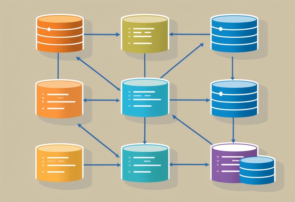
A series of interconnected tables representing different levels of normalization, with clear relationships and minimal redundancy

Database design using normalization techniques aims to organize data efficiently while ensuring data integrity and consistency. The design process focuses on structuring databases to prevent data anomalies.

Designing Databases with Normalization

Normalization is a key aspect of database design that divides large tables into smaller, more manageable ones.

This process reduces redundancy and dependency, which helps maintain data consistency across the system.

It involves organizing data into normal forms, each step refining and improving the structure.

Each normal form has specific rules to be followed. For instance, in the First Normal Form, all table entries must be atomic, with no repeating groups of data.

In the Second Normal Form, data must meet all the criteria of the First Normal Form, and each non-key attribute must depend on the table’s primary key.

Maintaining Data Integrity

Data integrity ensures that information within a database is accurate and reliable.

One crucial aspect is referential integrity, which involves maintaining consistency through relationships between tables. This prevents the entry of invalid data into a database by using foreign keys, ensuring all table references remain accurate.

Integrity constraints protect against unintended data loss or corruption.

Enforcing rules within the database management system ensures that operations align with business logic.

Strategies like transaction management further enhance consistency by treating operations as a single unit, ensuring all steps are completed successfully.

Implementing these measures preserves data quality, safeguarding against errors and aiding in long-term data management.

Normalization and SQL

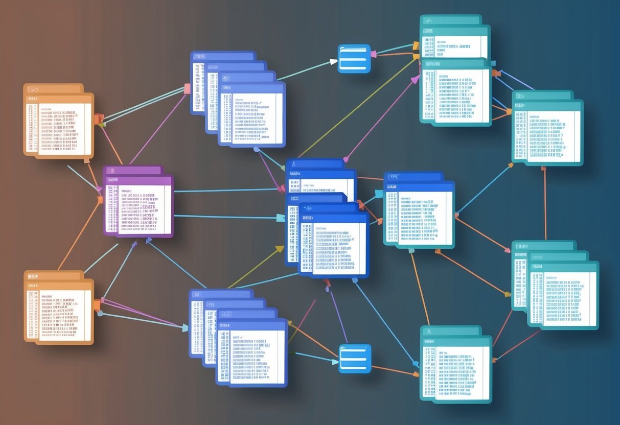
A series of interconnected tables representing data in various normal forms for a database, with arrows indicating relationships between them

Normalization in SQL is essential for organizing data efficiently. It involves structuring a database to minimize redundancy and improve data integrity.

By applying normal forms and optimizing SQL queries, databases can support fast, accurate data retrieval.

Applying Normal Forms in SQL

Normalization in SQL consists of several steps, each addressing different issues.

First Normal Form (1NF) requires each table column to hold only one value, eliminating repeating groups.

Second Normal Form (2NF) addresses partial dependency, ensuring every non-key attribute is fully dependent on the primary key.

Third Normal Form (3NF) removes transitive dependencies, where non-key attributes depend on other non-key attributes.

Foreign keys play an important role in this process, linking tables and maintaining referential integrity.

By enforcing relationships between tables, foreign keys help prevent anomalies.

SQL developers must be familiar with these concepts to design robust, scalable databases that support complex applications.

Familiarity with these normal forms is crucial for maintaining data consistency in systems like MySQL.

Writing Efficient SQL Queries

Efficient query writing in SQL is essential for maintaining performance, especially in large databases.

When queries are poorly constructed, they can slow down retrieval times significantly.

To enhance query performance, developers should focus on indexing.

Proper indexing can drastically reduce search times in large datasets, allowing for quicker access to needed data.

Moreover, eliminating unnecessary columns and joining only required tables can streamline SQL queries.

Using SELECT statements that target specific fields rather than retrieving entire tables can optimize operations.

SQL professionals should apply these techniques to ensure efficient data handling, keeping systems responsive and reliable.

Implementing these strategies helps manage data effectively across various platforms, including popular systems like MySQL.

Challenges and Trade-offs in Normalization

A series of interconnected puzzle pieces, each representing a different aspect of normalization, with varying levels of complexity and organization

Normalization in databases enhances data consistency and reduces redundancy. Yet, achieving the ideal level involves balancing flexibility and database performance. Understanding these aspects helps in making informed design decisions.

Analyzing Normalization Trade-offs

Normalization improves data integrity by organizing data into tables and ensuring dependability. Yet, this process can lead to slower query performance.

Joining several tables for a single query can increase complexity, affecting response time. As a result, designers often face challenges in optimizing performance.

Increased normalization might also reduce flexibility when future data requirements change.

Balancing these factors is key to effective database management.

Understanding how normalization impacts different system aspects helps. This includes evaluating performance bottlenecks and flexibility constraints.

It’s essential to weigh these considerations against potential benefits, such as data integrity and reduced redundancy.

Deciding on the Level of Normalization

Deciding on the appropriate level of normalization depends on various factors like the specific needs of a system.

While first normal form (1NF) eliminates repeating groups and ensures atomic values, higher forms, like third normal form, further delineate data relationships.

Yet, excessive normalization can lead to efficiency losses.

Choosing the correct level impacts how the database handles real-time applications.

While highly normalized databases reduce redundancy, they might not suit environments needing rapid query responses.

It’s important to assess the trade-offs between data redundancy and query speed, tailoring the normalization approach to the system’s demands, balancing both flexibility and performance.

Normalization in Practice

A series of three interconnected circles, each one smaller and inside the previous, representing the three normal forms of normalization

Normalization is a key process in organizing databases to reduce redundancy and improve data integrity. By structuring database tables effectively, normalization helps in efficient data management and facilitates easier database operations.

Real-world Normalization Examples

In many offices, customer databases are normalized to improve efficiency. For instance, a retail store might store customer details like name, address, and purchase history in different tables.

This ensures that updates to customer information are made only once, reducing errors and maintaining consistent data across the system. It simplifies queries by keeping data organized and helps in generating accurate reports.

Another example is in banking systems where transaction details, customer information, and account data need to be managed separately yet efficiently.

By normalizing these databases, banks can quickly retrieve and update specific data without the risk of altering unrelated information. This enhances security and speeds up transaction processes.

Normalization in Database Management Systems

Database Management Systems (DBMS) rely on normalization to maintain data quality.

In a DBMS, normalization involves organizing tables to ensure that they only store data relevant to each other.

For instance, in Database Normalization, tables must comply with rules of First Normal Form (1NF), Second Normal Form (2NF), and Third Normal Form (3NF) to eliminate redundancy.

By applying these rules in DBMSs, the systems reduce data anomalies and improve storage efficiency.

Each table has well-defined relationships, leading to easier maintenance and query optimization. This approach is essential in handling large datasets, ensuring that the information is accurate and easy to access without unnecessary duplication.

Frequently Asked Questions

A series of three interconnected gears, each labeled with "1NF," "2NF," and "3NF," symbolizing the process of normalization

Normalization in database management organizes data efficiently to minimize redundancy and maintain data integrity. These processes are essential for effective database design.

What is the purpose of normalization in a database management system (DBMS)?

Normalization helps structure data so each piece is stored only once. This reduces redundancy and ensures consistency. It also makes databases more efficient by organizing tables and relationships, supporting data integrity and ease of maintenance.

How does the first normal form (1NF) differ from the second (2NF) and third normal form (3NF)?

The first normal form (1NF) ensures each table cell holds a single value and each record is unique. The second normal form (2NF) adds that all non-key attributes must depend on the whole primary key. Third normal form (3NF) further requires that attributes are independent of non-primary key attributes.

Can you provide examples of tables in 1NF, 2NF, and 3NF?

A table in 1NF might list customer IDs and orders, ensuring each cell has a single value. In 2NF, this table would separate repeated data, like splitting order and customer data into distinct tables. In 3NF, it would also remove transitive dependencies, ensuring that all attributes depend directly on the primary key.

What are the steps involved in normalizing a database to the third normal form?

To reach the third normal form, start with 1NF by eliminating repeating data. Move to 2NF by ensuring each non-primary key attribute is fully dependent on the primary key. Finally, achieve 3NF by removing any dependencies between non-key attributes, ensuring everything is directly related only to the primary key.

How do the different normal forms impact the redundancy and integrity of data in a database?

As a database progresses through normal forms, redundancy is reduced. In 1NF, a table might still hold duplicate data. By 3NF, most redundancy is eliminated, contributing to higher data integrity. This ensures databases are easy to update, reducing the likelihood of inconsistencies.

Why is normalization important for efficient database design and what problems does it solve?

Normalization eliminates redundant data, which saves storage and reduces costs.

It simplifies database maintenance and supports robust data accuracy.

Problems like update anomalies are reduced as changes in data occur in fewer places, thus lowering the chance of inconsistencies.

Categories
Uncategorized

SSMS vs Azure Data Studio vs VS Code: Choosing the Right Tool for Your Data Management Needs

Comparing SQL Server Management Tools

When it comes to SQL Server management tools, three popular options are SQL Server Management Studio (SSMS), Azure Data Studio (ADS), and Visual Studio Code (VS Code).

SSMS is a comprehensive tool for managing different components of SQL Server. It offers advanced features for database administration.

Users who need detailed management capabilities often prefer SSMS.

Azure Data Studio is ideal for those who work across platforms. This tool is free and open-source.

It’s often favored by developers who need a modern, customizable interface. The tool supports SQL Server and Azure SQL Database.

Visual Studio Code caters to those who favor a lightweight application. Although primarily a code editor, it supports SQL queries through extensions.

This makes it flexible for users who work with multiple programming languages.

Let’s compare some features in a simple table:

Feature SSMS Azure Data Studio VS Code
Platform Support Windows Cross-platform Cross-platform
IntelliSense Basic Advanced Via extensions
Extensions and Add-ons Limited Extensive Extensive
Administration Tools Advanced Basic Basic

This comparison shows how different tools cater to varied needs in SQL Server management. Each tool has its strengths, and the best choice often depends on the specific requirements of the user.

Supported Operating Systems

Three computer screens side by side displaying SSMS, Azure Data Studio, and VS Code interfaces. Icons and windows open on each screen

SQL Server Management Studio (SSMS), Azure Data Studio, and Visual Studio Code have different compatibility with operating systems. Understanding these differences can help users choose the right tool for their needs.

Windows Compatibility

SSMS is primarily designed for Windows. It’s a tool many database administrators rely on, but it does not support other operating systems like Linux or macOS. This limits its use for those who work across different systems.

Azure Data Studio and Visual Studio Code, however, both support Windows. They provide a flexible environment for users who prefer using Windows but need a tool that can also support other platforms.

For users solely on Windows, any of these options would work, though their additional features should be considered based on user needs.

Linux and MacOS Support

For users on non-Windows platforms such as Linux and macOS, Azure Data Studio and Visual Studio Code offer strong compatibility.

Azure Data Studio is notable for its cross-platform support, making it a preferred choice for developers needing flexibility in operating systems. It allows users to have a consistent experience across different machines.

Visual Studio Code, a favored tool among programmers, also works well on Linux and macOS. Its open-source nature and wide range of extensions increase its adaptability.

SSMS falls short here, restricting use to Windows, which can be a decisive factor for professionals who need a cross-platform solution. For more on this, visit how Azure Data Studio is supported on various platforms.

User Interface and Experience

Choosing the right SQL management tool often depends on the user interface and overall experience. Azure Data Studio, SSMS, and VS Code each offer unique features in terms of design, accessibility, and customization.

Graphical Interface Design

Azure Data Studio is designed with a modern and streamlined interface, which includes a dashboard that offers widgets for quick insights and reports.

It draws from Microsoft’s Visual Studio Code, providing a familiar environment for those acquainted with this editor. Dark mode is a popular feature and is easily enabled, enhancing readability and reducing eye strain.

By contrast, SSMS adopts a more traditional layout, which appeals to seasoned SQL professionals accustomed to a classic look and feel. Meanwhile, VS Code is robust with extensions, supporting a wide range of programming tasks beyond SQL.

Accessibility Features

Accessibility in these tools plays a key role, especially for developers who require specific accommodations.

Azure Data Studio shines with its native cross-platform compatibility, allowing use on Windows, macOS, and Linux. It integrates tools that aid in collaborative editing, making it suitable for diverse teams.

SSMS, while more traditional, excels with its comprehensive database management capabilities, though it primarily runs on Windows.

VS Code is noted for its extensibility and offers many plugins that enhance accessibility, catering to developers with different needs and preferences.

Customization Options

Azure Data Studio offers significant customization opportunities with a wide array of extensions and themes available, providing flexibility to tailor the workspace. It supports Markdown and Jupyter notebooks, offering users diverse ways to document and present data.

SSMS focuses more on in-depth administrative functions rather than customization; it has fewer options but remains highly effective for managing SQL Server environments.

VS Code stands out in customization, with thousands of extensions and themes, allowing users to configure almost every aspect of their interface to optimize productivity and functionality.

Development and Administration Features

SQL Server Management Studio (SSMS), Azure Data Studio, and Visual Studio Code (VS Code) each offer distinct features valuable for database development and management. Whether focusing on coding efficiency or robust database administration, these tools cater to different requirements for developers and database administrators (DBAs).

Advanced Database Development

SSMS is known for its powerful query editor, enabling developers to write and test complex SQL queries. With its integrated graphical tools, it suits those who prefer a traditional IDE for database development.

The Object Explorer in SSMS provides an organized view of database objects, making navigation intuitive for developers working on large databases.

Azure Data Studio is ideal for those seeking a cross-platform tool. Its modern interface supports a more streamlined development experience.

With built-in Git integration and the integrated terminal, developers can manage version control directly within the tool. This setup fosters seamless collaboration and simplifies the development workflow, especially for those incorporating continuous integration practices.

VS Code offers flexible extensions for SQL development. While not specifically a database management tool, its comprehensive extension library allows developers to customize their workspace for SQL needs. This flexibility benefits developers who juggle multiple programming environments or prefer lightweight setups.

Efficient Data Management

Azure Data Studio excels in data management with its lightweight structure and innovative features. It supports connectivity to various databases, both cloud and on-premises, facilitating scripting and data file manipulation. The user-friendly dashboards and customizable insights allow developers to efficiently track performance metrics.

In SSMS, data management is robust, offering extensive tools for import/export operations. The Query Editor is complemented by multiple built-in templates and code snippets, helping create standardized queries quickly. This feature-set appeals to enterprises needing structured data management protocols.

VS Code also supports data management through extensions, providing basic query running capabilities. This environment suits those who want to handle SQL tasks without using a dedicated database manager, merging development and simple data management in one tool.

Database Administration and Maintenance

SSMS stands out with its comprehensive suite for database administration. Features like backup and restore operations, detailed performance tuning aids, and security management options are vital for DBAs.

Its capacity to handle advanced database administration tasks makes it a preferred choice for those responsible for maintaining database health and reliability.

For Azure Data Studio, the focus is on flexibility and modern needs. It offers decent database administration capabilities, though it may lack some advanced functionalities found in SSMS. The extensions available for Azure Data Studio enhance its base features, particularly for developers focused on modern deployment models.

VS Code, while not primarily a tool for database administration, offers essential functionalities through extensions that allow users to perform maintenance tasks on databases. Its adaptability means users can tailor it to meet basic administrative needs, useful for lightweight or non-enterprise scenarios where database upkeep is necessary.

Extensibility and Integration

A cluttered desk with three open laptops, each displaying a different coding environment: SSMS, Azure Data Studio, and VS Code. Various cables and devices are scattered around the workspace

Each tool—SSMS, Azure Data Studio, and VS Code—has its own approach to enhancing usability through extensibility and integration features. They allow users to customize their environment with extensions and plugins, support version control, and offer compatibility with various programming languages, enhancing their utility and flexibility.

Adding and Managing Extensions

Azure Data Studio and VS Code both stand out for their ability to add and manage extensions. Users can browse and install a vast library of extensions to tailor these tools to specific needs, such as integrating Jupyter Notebooks or additional SQL Server management functions.

With VS Code, the process is incredibly straightforward, and users have access to a wide array of plugins. This makes it adaptable for different tasks such as managing databases or working with various programming environments.

SSMS, on the other hand, is more limited in this aspect. It does not offer the same level of extensibility through third-party plugins, focusing instead on providing a comprehensive set of built-in features tailored for SQL Server administration.

Version Control Integration

Both Azure Data Studio and VS Code provide robust version control integration, crucial for managing code changes and collaboration.

Azure Data Studio integrates source control effectively, offering a modern editing experience with its source control integration.

VS Code excels with its seamless integration with Git, allowing users to commit, push, and track code changes without leaving the editor. This makes it an ideal choice for development teams who require frequent code updates and collaboration.

SSMS lacks built-in source control features, which may necessitate external tools for version management. Users working primarily with databases may find this sufficient, but developers frequently collaborating on code projects might prefer the integrated approach of Azure Data Studio or VS Code.

Support for Programming Languages

Regarding programming languages, VS Code is exceptionally versatile, supporting numerous languages like Python and Scala. Its open-source nature ensures that language support continues to grow through community and official extensions.

Azure Data Studio also supports various languages and can be extended to work with languages like Python, especially useful for data science applications through its integration with Jupyter Notebooks.

SSMS, while primarily focused on SQL, offers some scripting capabilities. However, it doesn’t support the variety of programming languages found in VS Code or Azure Data Studio, making these alternatives preferable for users needing a multi-language environment.

Collaborative and Advanced Features

Three software logos displayed side by side with various icons and features surrounding them

When comparing SSMS, Azure Data Studio, and Visual Studio Code, it’s important to explore their support for data science, machine learning, security tools, and performance optimization. Each tool offers unique features that enhance teamwork and efficiency for developers and database administrators.

Data Science and Machine Learning Support

Azure Data Studio supports data science and machine learning with Jupyter Notebooks. These interactive notebooks allow users to write and run code, visualize data, and document workflows within a single environment.

This feature is beneficial for those involved in data analysis and machine learning projects. In contrast, SSMS does not natively support Jupyter Notebooks, which can limit collaboration in data science tasks.

Visual Studio Code, while versatile, does not include built-in features for data science but supports extensions that enhance its capabilities.

For users focused on data science, Azure Data Studio’s integration with Jupyter Notebooks provides a more tailored experience. This emphasis on data science makes it a strong choice for teams working on machine learning projects.

High Availability and Security Tools

SSMS excels in providing advanced security and high availability tools essential for enterprise environments. It includes features like Always On for high availability and Always Encrypted for enhanced data security.

These tools help in maintaining data integrity and availability, making SSMS suitable for environments where security and reliability are critical.

Azure Data Studio, while modern and user-friendly, lacks some of these built-in high availability and security features. Users may need to rely on external tools or additional scripts to achieve similar security standards.

Performance Insights and Optimization

Performance monitoring and optimization are crucial, and both SSMS and Azure Data Studio cater to these needs differently.

SSMS provides extensive performance monitoring tools like Performance Insights and SQL Server Reporting Services (SSRS) to analyze and optimize SQL queries effectively. These tools are vital for database administrators who aim to ensure optimal resource usage and database speed.

Azure Data Studio, although lacking some of SSMS’s advanced performance tools, offers extensions and integrations that help in query performance insights. It enables users to optimize their queries and manage database workloads efficiently.

Developers using Visual Studio Code can enhance their experience through extensions, though it demands more manual configuration for performance tasks compared to SSMS.

Frequently Asked Questions

A table with three laptops open, each displaying the interfaces of SSMS, Azure Data Studio, and VS Code

Azure Data Studio, SSMS, and Visual Studio Code are powerful tools for managing SQL databases. Each offers unique features and is suitable for different use cases.

What are the differences between Azure Data Studio and SSMS?

Azure Data Studio is a modern, lightweight tool that supports cross-platform use, making it a good choice for working on macOS or Linux. It is built on top of the Visual Studio Code platform and provides an extensible interface.

In contrast, SSMS offers advanced administrative features, ideal for managing SQL Server environments on Windows.

Is Azure Data Studio compatible with SQL Server Management Studio extensions?

Azure Data Studio does not support SQL Server Management Studio extensions directly. It has its own set of extensions developed for its unique ecosystem. This tool is geared more toward cross-platform versatility and editing, unlike SSMS, which is focused on comprehensive administrative functions.

Can Visual Studio Code be used effectively for SQL database management tasks?

Visual Studio Code, with the right extensions, can be a handy tool for SQL database tasks. It offers a flexible environment where developers can tailor it to their needs, focusing on coding and lightweight editing.

This makes it a popular choice for those who appreciate the extensibility and interface similar to Azure Data Studio.

What are the pros and cons of using Azure Data Studio compared to other database tools?

Azure Data Studio shines with its cross-platform capabilities and modern UI, making it appealing to developers who need a simple, adaptable tool. However, it lacks some advanced features present in SSMS. Developers need to weigh the simplicity and development focus of Azure Data Studio against the comprehensive management features of other tools.

How does performance in Azure Data Studio compare with SSMS for typical database management tasks?

In terms of performance, both tools cater to different aspects of SQL management.

Azure Data Studio is optimized for querying and lightweight tasks, while SSMS is robust, offering deep integration and advanced features for complex database management. Users should consider the nature of their tasks when choosing between these tools.

What features differentiate Visual Studio Code when used with SQL-related extensions from Azure Data Studio?

Visual Studio Code stands out with its flexibility and support for a wide range of extensions, allowing users to configure it according to their specific needs.

In comparison, Azure Data Studio, while also built on Visual Studio Code, is more specialized for database management.

This specialization may limit its use in broader development tasks but makes it a strong option for SQL-focused work.

Categories
Uncategorized

Learning Power BI – Data Prep: Mastering Data Extraction and Transformation

Overview of Power BI

Power BI is a powerful tool that supports data analysis and visualization. It allows users to create reports and dashboards, simplifying data interpretation and enabling informed decision-making. The platform includes several core components, with Power BI Desktop being a key area of focus for creating custom visualizations and data models.

Introduction to Power BI Desktop

Power BI Desktop is a robust application that acts as the starting point for building and designing reports. It provides tools for importing data from various sources, including Excel, databases, and online services.

Users can clean and transform the data to fit their needs.

In Power BI Desktop, users have the flexibility to use self-service data prep tools, enabling quick data shaping and modeling. This feature makes it easier to create detailed reports and insightful data analysis.

Drag-and-drop functionality enhances user experience, allowing for intuitive report creation and customization.

Furthermore, Power BI Desktop supports the creation of interactive visualizations. These can be tailored with custom visuals, improving the clarity of reports and dashboards, as explained in Power BI Data Modeling.

Core Components of Power BI Ecosystem

The Power BI ecosystem consists of several interconnected tools and services. These include Power BI Desktop, Power BI Service, and Power BI Mobile apps. Each plays a vital role in data management and collaboration. The Power BI Service is an online platform where users publish and share reports, making collaboration seamless.

Dashboards in the service provide a consolidated view of key metrics and insights. They compile visualizations from multiple reports, enabling easy tracking of important data.

As part of the ecosystem, Power BI also offers options for real-time data streaming, enhancing its capability for time-sensitive data analysis.

Data connectivity is another important aspect, with Power BI connecting to a wide array of sources. This versatility allows users to build comprehensive models and dashboards, supporting diverse business needs. For more details, refer to a comprehensive discussion in Learning Microsoft Power BI.

Sourcing Data

Understanding how to source data effectively is essential for making the most out of Power BI. This section explores various data sources, the impact of connectivity types, and the use of dataflows, as well as the integration of big data and cloud sources.

Identifying Various Data Sources

Data sources are crucial for building insightful Power BI reports. They can range from relational databases like SQL Server and Oracle to NoSQL data stores such as MongoDB. Understanding these sources helps analysts choose the right data for their analysis.

Identifying the characteristics of each data source is vital. Consider aspects like data format, update frequency, and connection requirements.

Knowing these can optimize data preparation and ensure efficient data retrieval in Power BI.

Connectivity Types and Their Impact

Connectivity types can significantly affect data performance and management. There are two main connectivity types in Power BI: import and direct query. Choosing between them depends on the data size and refresh needs.

Import mode allows data to be loaded into Power BI, making it faster for analysis but requiring regular updates.

Direct query, on the other hand, keeps data in the source, allowing for real-time updates but might impact performance.

Selecting the right connectivity type is critical for balancing performance and data freshness.

Utilizing Power BI Dataflows

Power BI dataflows provide a way to process and clean data within Power BI itself. They allow users to create reusable data preparation logic, which saves time and effort.

Dataflows can be linked to various data sources and help in shaping and transforming data using the Power Query editor. This makes it easier to maintain consistent data transformation steps across multiple reports and dashboards.

Dataflows are especially useful when dealing with complex data transformations or when working with multiple data sources consistently.

Incorporating Big Data and Cloud Sources

Big data and cloud sources are increasingly important in the modern data landscape. Integrating these into Power BI requires understanding both the type of cloud service and the data source characteristics.

Services like Azure, AWS, and Google Cloud offer scalable solutions for storing and retrieving large datasets.

Power BI supports connections to these cloud sources, allowing users to harness the power of big data analytics efficiently.

When working with these sources, consider factors such as data privacy, access speed, and cost to make informed decisions.

Data Extraction Techniques

Data extraction is a crucial step in preparing data for analysis in Power BI. Techniques such as loading data from Excel, connecting to databases like SQL Server, and using ETL processes are essential.

Retrieving Data from Microsoft Excel

Excel is a common tool for data storage and manipulation. Retrieving data from Excel into Power BI allows users to leverage familiar data structures.

Users can import entire sheets or specific ranges, making it flexible for both small and large data sets. Formatting and cleaning data before loading can save time.

Techniques like using named ranges and structured tables help in maintaining consistency. Enabling auto-refresh ensures data is up-to-date, reducing manual updates.

Connecting to SQL Server and Other Databases

SQL Server is a powerful database system used widely in businesses. Power BI can easily connect to SQL Server, allowing users to retrieve large volumes of data efficiently.

This connection supports data exploration and transformational capabilities directly. By using SQL queries, users can filter and preprocess data before it arrives in Power BI.

Other databases like MySQL and Oracle can also be connected similarly, providing versatile data access. Ensuring secure and optimized queries is important to prevent performance problems and ensure data integrity.

Implementing ETL Process for Data Preparation

ETL (Extract, Transform, Load) is a core process in data preparation. It involves extracting data from various sources, transforming it into a suitable format, and loading it into Power BI.

Tools like SSIS and Azure Data Factory enhance ETL process efficiency. Transformations include cleaning data, aggregating information, and adjusting formats.

Data integration from multiple sources is also facilitated during transformation, improving analysis quality.

Using Power BI’s Query Editor, users can implement ETL processes for streamlined data handling, ensuring that only quality data is analyzed.

Transforming and Shaping Data

Transforming and shaping data in Power BI involves adjusting raw data to make it more useful for analysis. This process includes using tools like Power Query to make data more reliable and informative by cleaning, pivoting, and renaming elements.

Using Power Query for Data Transformation

Power Query is a powerful tool used for data transformation. It helps users to import data from various sources, such as Excel, databases, and web pages.

Once the data is loaded, Power Query provides options to transform it by removing unnecessary columns, filtering rows, or merging tables. The Advanced Editor allows for more complex transformations through custom M code.

Users can easily rename and pivot data to better suit their needs. Power Query also lets users group data, which can help to summarize and analyze information effectively.

These features enhance the data preparation process, making Power Query an essential tool for any analytical task.

Essentials of Data Cleaning and Profiling

Data cleaning and profiling are crucial for ensuring the quality and reliability of data. Profiling involves checking data quality by identifying issues like duplicates, missing values, or inconsistent data formats. These checks help users assess the accuracy and completeness of data before further analysis.

In Power BI, data cleaning tasks like removing duplicates, correcting errors, and filling in missing values are simplified with Power Query. Profiling tools also allow users to profile columns, which helps in understanding the data distribution and spotting anomalies.

Implementing these cleaning steps ensures that the data conforms to the standards required for accurate business reporting and analysis.

Advanced Data Shaping Techniques

Advanced data shaping techniques involve more complex operations to tailor data for specific needs. Power Query supports these operations with features like transposing tables, creating custom columns, and conditional column generation.

This flexibility allows data to be molded into a format that maximizes its analytical potential.

To further refine data, users can apply rule-based transformations that automatically adjust values based on certain conditions. Another advanced technique is the integration of data from multiple sources, which improves the depth of analysis.

These advanced shaping methods elevate a user’s ability to produce customized data models that are directly aligned with their analytical objectives.

Data Modeling Essentials

Data modeling is crucial for turning raw data into organized, actionable insights in Power BI. It involves understanding how data points connect and optimizing data performance. Attention to relationships and granularity ensures accuracy and efficiency.

Understanding Relationships and Data Granularity

In data modeling, recognizing relationships between different data tables is vital. These relationships define how data connects across sources. Whether in a business intelligence guidebook or practical applications, they are the backbone of an effective data model.

Data granularity refers to the level of detail stored in the model. It affects how detailed the analysis can be. Fine-grained data allows for more detailed insights, while coarse granularity provides broader overviews.

A careful choice of granularity helps data analysts balance storage and performance challenges effectively, ensuring that reports and dashboards meet user needs.

Optimizing Data Models for Performance

Performance in data models significantly impacts the speed and efficiency of Power BI reports. To achieve optimal performance, data analysts often use the right storage mode.

Import mode is suitable for fast queries with medium data volume. Meanwhile, DirectQuery is better for large datasets but may slow down performance.

Data model optimization includes removing unnecessary columns and tables, reducing model size, and ensuring column data types are appropriate. Techniques like aggregations and indexing can further enhance performance.

Properly optimizing data wrangling techniques ensures that the model remains efficient, scalable, and user-friendly.

Loading and Storage Considerations

Loading data efficiently and choosing the right storage options are crucial when working with Power BI. These choices impact performance and data management.

Choosing the Correct Storage Mode

Selecting the right storage mode can greatly affect both performance and flexibility. Power BI offers several storage modes such as Import, DirectQuery, and Dual.

  • Import Mode stores a copy of the data within Power BI, offering excellent performance. It’s suitable for smaller datasets where speed is essential.
  • DirectQuery Mode connects directly to the data source, useful for handling large datasets that change frequently. Though it can slow down report performance, it ensures up-to-date data.
  • Dual Mode allows for hybrid scenarios, where some tables are imported while others use DirectQuery. This mode provides a balance between performance and data freshness.

Deciding on the right mode depends on the dataset size, performance requirements, and data timeliness.

Strategies for Incremental Refresh

Incremental refresh is key to improving the performance of large datasets in Power BI. It enables the update of only new or changed data, not the entire dataset.

  • Establishing a refresh policy is vital. This policy defines parameters such as how often and what data range should be refreshed.
  • Using partitioning helps manage data efficiently. Data is split into partitions, which reduces load times by only refreshing specific parts.

Implementing incremental refresh is beneficial in scenarios where data changes frequently but historical data remains constant. This strategy saves time and reduces load, enhancing overall performance.

Advanced Data Analysis

Advanced data analysis in Power BI leverages complex techniques and custom measures to provide deep insights. With methods like time series analysis, users can forecast trends and enhance predictive modeling. Custom measures expand analytical capabilities by building unique calculations for more detailed datasets.

Time Series Analysis Techniques

Time series analysis is essential for predicting and understanding data trends over time. It involves examining patterns such as seasonality, cycles, and trends.

In Power BI, users can utilize time series analysis to forecast future values using custom visuals and DAX formulas. Techniques like exponential smoothing help in smoothing out noise for clearer trend visualization.

Time series analysis often requires cleaning and preparing data since missing data points can significantly impact results. When using Power BI, connecting to varied data sources ensures comprehensive datasets for more accurate forecasting.

Implementing these techniques can lead to enhanced decision-making and strategy development by identifying patterns and projecting future trends.

Achieving Deeper Analytics with Custom Measures

Custom measures in Power BI allow users to perform calculations that standard aggregations do not cover. By using Data Analysis Expressions (DAX), users can create custom calculations tailored to their unique needs.

This capability is crucial for organizations needing in-depth insights from their data.

Creating custom measures requires understanding both data structures and logic expressions. They can be used to calculate percentages, averages, or any specific metric needed for detailed analysis.

Custom measures enable businesses to interpret their data more effectively, driving informed decisions by transforming raw data into actionable insights.

Users leverage these tools in Power BI to push beyond basic analysis, achieving a deeper understanding of complex data sets and improving analytical outcomes.

Data Quality Assurance

A computer screen displaying various data sources being connected and shaped in Power BI

Ensuring the quality of data is crucial in Power BI data preparation. It involves detecting anomalies and profiling columns to maintain data integrity. Sufficient attention to these aspects enhances the reliability of analysis and insights.

Detecting and Handling Data Anomalies

Data anomalies can lead to incorrect analysis and reporting. Detecting these outliers is crucial to maintain data accuracy.

Various methods like visual inspection, statistical analysis, and automated tools help identify anomalies. Tools can compare expected patterns with actual data, highlighting discrepancies.

Once detected, handling anomalies involves deciding whether to correct, omit, or transform the data.

  • Data correction includes fixing errors in data entry or format.
  • Omission may be necessary when anomalies cannot be clarified or verified.
  • Sometimes, it might be suitable to transform data through processes such as normalization to ensure consistency across datasets.

Profile Columns to Ensure Data Integrity

Profiling columns helps understand data structure and quality. It involves analyzing each column’s statistical properties, such as mean, median, and frequency of values. This insight can reveal inconsistencies or missing values, impacting results.

Column profiling tools can automatically generate summaries, making it easier to spot issues like duplicate entries or unusual value distributions.

They ensure each column aligns with expected data standards, improving overall data integrity.

Profiling helps identify potential data quality issues, allowing data handlers to address them before proceeding to analysis or visualization. Adjusting for these discrepancies upfront can prevent misinterpretations of the data.

Sharing and Collaboration in Power BI

In Power BI, collaborating with team members and sharing insights through reports and dashboards is essential for effective data analysis. This section explores the functionalities of Power BI, including the workspace environment and how to create shareable content efficiently.

Working with Power BI Workspace

The Power BI Workspace acts as a central hub for managing all reports and dashboards. It allows users to collaborate in real-time, making it easier for teams to access and work on shared projects.

Each workspace can host multiple datasets and reports, which helps in organizing content based on specific projects or departments.

Users can set permissions to ensure that only authorized personnel access sensitive information. This is vital for maintaining data security while enabling collaboration.

Teams can have different workspaces tailored to distinct projects, adding flexibility and structure to data management.

Collaboration is enhanced through Power BI’s integration with other tools, such as Microsoft Teams. This allows users to discuss reports and make changes without leaving the workspace. Sharing feedback or suggesting modifications directly within the platform streamlines the collaborative process.

Creating Shareable Reports and Dashboards

Creating shareable reports and dashboards in Power BI is straightforward and enhances the decision-making process across an organization.

Reports are crafted using various visualization tools that help present data in an understandable way. Meanwhile, dashboards provide a snapshot of important metrics, allowing users to monitor performance efficiently.

Once a report or dashboard is ready, it can be easily shared via direct links or through embedding in other applications.

Power BI also supports publishing to the web, making findings accessible to a broader audience if needed.

This feature is beneficial for teams that collaborate with external partners or clients.

Adding a shareable certificate can provide additional validation and security, ensuring the integrity and authenticity of shared data. This enhances trust among users and stakeholders, particularly when dealing with critical business information.

The ability to share and collaborate effectively in Power BI aids in fostering a data-driven culture within organizations.

Leveraging BI Tools for the Digital Economy

In today’s digital economy, business intelligence (BI) tools are crucial for making informed decisions. Microsoft Power BI is an essential tool, combining data from different sources and transforming it into actionable insights.

Data analytics plays a pivotal role in this process. Power BI allows users to clean and visualize data, making it easier to identify trends. This can significantly enhance decision-making and strategic planning for businesses.

To leverage these tools effectively, businesses should focus on integrating their data sources. Power BI supports various data sources like Excel, SQL databases, and cloud services, providing flexibility in data handling.

Benefits of Using Power BI in the Digital Economy:

  • Data Connectivity: Power BI connects to various data sources seamlessly.
  • Interactive Dashboards: Users can create interactive dashboards that update in real-time.
  • User-Friendly Interface: With a focus on simplicity, Power BI is accessible to users with varying expertise.

By using BI tools, companies can adapt quickly to market changes. This is due to the enhanced ability to analyze large datasets. Companies can stay ahead by identifying opportunities and managing risks effectively.

In the rapidly evolving digital landscape, leveraging tools like Power BI empowers organizations to drive growth and maintain a competitive edge.

Professional Development in Power BI

Engaging in professional development for Power BI involves acquiring certifications and practical experience. These elements enhance skills, making individuals more competitive in the field of data analysis.

Earning Career and Shareable Certificates

Career certificates in Power BI can boost job prospects for data analysts. Certificates are available through various platforms, offering structured courses that cover essential skills like data visualization and analysis.

Completing these programs often results in a shareable certificate, which can be displayed on professional networks like LinkedIn. These certificates validate one’s expertise and can differentiate candidates in a crowded job market.

Aside from career advancement, they also ensure professionals stay updated with the latest tools and features in Power BI, contributing to continuous learning and growth.

Engaging in Hands-On Projects and Learning

Hands-on projects are crucial for mastering Power BI. Practical experience allows individuals to apply theoretical knowledge in real-world scenarios.

Engaging in projects that simulate workplace situations helps develop problem-solving skills. These projects might involve importing data from different sources, shaping data, and creating dashboards.

By participating in hands-on learning, professionals gain confidence in using Power BI tools, making them ready for challenges in data analysis roles.

It’s also a way to demonstrate skills during job interviews, as completed projects can be showcased in portfolios. Regular practice through these projects ensures that learning goes beyond just theoretical concepts, embedding practical understanding.

Online Learning Resources

A person at a desk with a computer, accessing various data sources and shaping data in a Power BI learning module

Online learning offers a convenient way to gain skills in Microsoft Power BI. Two important platforms are Coursera and Coursera Plus, providing a range of courses on data analytics and data preparation techniques.

Utilizing Coursera for Power BI Training

Coursera hosts numerous courses focused on Microsoft Power BI, which cater to both beginners and advanced users. These courses often cover essential skills like data loading, transformation, and visualization.

Students can access video lectures, quizzes, and peer-reviewed assignments.

A notable feature is the flexibility offered by Coursera. Learners can study at their own pace, fitting study time around existing commitments. For those seeking broader insights, Coursera also integrates learning paths covering multiple aspects of data analytics.

Exploring Power BI Courses on Coursera Plus

Coursera Plus provides unlimited access to thousands of courses, including those on Power BI. This subscription model is ideal for learners who wish to explore multiple courses without worrying about individual costs.

Subscribers can delve into complex skills like DAX (Data Analysis Expressions) and Power Query. The variety of courses helps cater to different learning styles, ensuring that learners can find resources suited to their preferences and needs.

This platform is beneficial for those who intend to deepen their understanding of data analytics, beyond just the basics of Power BI. More courses on data sciences and related areas are also available to complement their Power BI knowledge.

Frequently Asked Questions

Understanding how to handle data in Power BI is crucial for effective analysis. This guide answers common questions about combining tables, data cleaning, loading, and integrating data from various sources. It also explores tools within Power BI for managing queries.

How can you combine tables with the same columns in Power BI?

In Power BI, users can combine tables by using the “Append Queries” feature. This is useful when all tables have the same structure. After appending, it’s important to check for any duplicate entries or data inconsistencies.

What are the best practices for data cleaning in Power BI?

To clean data efficiently, users should first remove any duplicates and correct errors. Then, they should ensure accurate data types for each column. Utilizing Power Query Editor can streamline this process and help create repeatable cleaning steps.

How do you prepare and load data for analysis in Power BI?

Preparing data in Power BI involves importing it using Power Query Editor. Once the data is shaped as needed, it can be loaded into the model. Just make sure to optimize the model for analysis to improve performance.

What steps are involved in cleaning and transforming data in Power BI?

Data transformation in Power BI starts with removing null values and handling missing data. Users can then reshape the data by pivoting or unpivoting columns. Adding custom columns or calculated fields enhances the dataset.

How can you get and integrate data from various sources into Power BI?

Power BI supports integration from diverse sources like Excel, databases, and web services. Users can connect to these sources directly within Power BI and use Power Query Editor to shape the data for their needs.

What tools are available within Power BI to consolidate and manage queries?

Power BI offers the Power Query Editor for managing queries. This tool allows users to consolidate data from different tables and apply transformations. Users can also use advanced features like M Language to create more complex query operations.

Categories
Uncategorized

Learning About Python Scope: A Comprehensive Guide

Understanding Python Scope Fundamentals

Python scope determines where variables can be accessed within the code. It is essential for developers to grasp how Python handles variable visibility by using different scopes, following the LEGB rule.

The Four Scopes in Python: LEGB

In Python, variables can exist in four main scopes: Local, Enclosing, Global, and Built-in. These scopes are often referred to using the acronym LEGB. This structure defines the sequence that Python follows when checking where a variable is defined or can be accessed.

  • Local Scope: Variables within a function. They can only be accessed inside that function.
  • Enclosing Scope: This applies to nested functions. Variables in the outer function are accessible to the inner function.
  • Global Scope: These variables are defined at the top level and are accessible throughout the module.
  • Built-in Scope: Contains special Python-provided functions and names that are always available.

Understanding these scopes ensures that developers know where and how variables can be accessed in a program. For detailed insights, explore the LEGB Rule in Python Scope.

Variable Scope and Accessibility

The scope affects a variable’s accessibility, meaning where it can be used in the program.

For instance, local variables are restricted to the block they are created in, such as a function or loop. This ensures variables don’t interfere with others outside their scope.

With global variables, accessibility extends to the entire module. If accessed within a function, Python first looks for local variables before searching globally. The rules of accessibility defined by LEGB help avoid conflicts and unexpected errors in the code.

By following the principles of Python scope, programmers can manage variables effectively, preventing unintended changes in data and maintaining code clarity.

Global and Local Scopes Explained

Python’s scope rules determine where variables can be accessed within the code. Understanding these scopes is crucial for managing variables effectively and avoiding errors.

Defining Global Scope

In Python, the global scope refers to variables that are declared outside any function. These variables are accessible from any part of the code, both inside and outside functions. Global variables can be useful when the same data needs to be accessed throughout a program. For example, setting a variable like config = True outside a function makes config available everywhere.

However, modifying global variables inside functions requires the global keyword. This tells Python to use the variable from the global scope, instead of creating a new local one. For instance, updating a variable within a function would involve declaring it as global variable_name. Though global variables offer flexibility, overusing them can lead to issues with code readability and debugging.

Understanding Local Scope

Local scope refers to variables defined within a function. These variables exist only during the function’s execution and cannot be accessed outside of it. This isolation helps prevent conflicts with variables in other parts of the program.

If a variable like total = 10 is created inside a function, it is a local variable.

Each time a function is called, its local scope is created anew, ensuring that variables do not overlap between calls. This makes local variables ideal for temporary data that is specific to a function’s task. Using local variables keeps the program organized, as they are confined to the function in which they are declared, enhancing modularity and maintainability. For more on local scope, explore the concept on the Programiz site.

The Global Keyword in Depth

The global keyword in Python is essential for modifying variables outside their local scope. It allows programmers to alter global variables from within functions, impacting how data is organized and accessed across the program.

Usage of the Global Keyword

In Python, the global keyword is used within a function to change variables at the global scope. This means variables can be modified outside their local environment, which is typically restricted.

Using global, a function can create or alter global variables. This is useful when a variable needs to be changed in multiple functions or modules. Code examples, like those found in examples at W3Schools, demonstrate how a global declaration can alter a global variable from within a function.

The global keyword ensures that when a variable is called, Python recognizes it as global. This avoids confusion with variables that might share the same name but are local to other functions. Examples show it simplifies data management, though care is needed to prevent unintended changes.

Implications of Global Variable Assignment

Assigning variables as global means storing them in the global namespace. This impacts how variables are accessed throughout the program.

Global variables can be used by any function, making them powerful but also posing risks.

Global variables can lead to increased program complexity. If many functions modify the same global variable, it becomes difficult to track changes and debug issues. Solutions may include limiting the use of global state or isolating global variables to key functions.

It’s also advisable to document when and why global variables are used. This helps maintain clarity in codebases, as seen in in-depth discussions of global scope. Properly used, the global keyword balances accessibility and control within Python programs.

Delving Into Enclosing and Nested Scopes

Enclosing and nested scopes are crucial in Python programming. They determine how variables are accessed within functions and impact code organization. Understanding these concepts helps avoid errors and makes the code cleaner.

Nested Functions and their Scopes

Nested functions occur when a function is defined inside another function. In Python, this structure allows the inner function to access variables in the outer function’s scope. This is known as a nested scope. These inner functions can modify or use the surrounding variables, enabling more complex and organized code.

Nested functions are particularly useful for closures, which capture and remember values from their enclosing function even after the outer function has finished executing.

Nested scopes follow Python’s LEGB rule, prioritizing Local, Enclosing, Global, and Built-in scopes. It is essential for programmers to understand how this hierarchy affects variable access.

By using nested functions, developers can hide details and create more modular code, enhancing readability and maintainability.

Enclosing Scope Mechanics

The enclosing scope refers to the environment a nested function inherits from its containing function. It allows variables from the outer function to be used within an inner function without needing to pass them as arguments.

This capability is established through Python’s nonlocal keyword, which enables the inner function to modify variables from its enclosing scope.

Enclosing scopes are significant as they allow maintaining state across function calls with minimal overhead, often used in decorator functions or when defining callbacks.

Recognizing the enclosing scope helps in debugging scope-related issues by clarifying where variables are defined and modified. If a variable isn’t found in the local scope, Python automatically checks the enclosing scope level, providing a flexible variable access system for complex programs.

The Nonlocal Keyword and Its Use Cases

The nonlocal keyword in Python is crucial for managing variable scopes, especially in nested functions. It allows variables to be shared across these nested scopes without affecting global variables.

When to Use Nonlocal Keyword

In Python, the nonlocal keyword is used within nested functions when there is a need to modify a variable defined in an enclosing scope. This is important when a function needs to modify a variable from its enclosing function without making it a global variable.

For example, in a function-within-a-function setup, if the inner function needs to update a counter variable from the outer function, nonlocal can be employed. By doing so, the outer function’s state can persist across multiple calls to the inner function.

When the nonlocal keyword is used, Python searches for the variable in the nearest enclosing scope rather than the global scope, enhancing efficiency and clarity in code design.

Differences Between Nonlocal and Global

The distinction between nonlocal and global is found in their scope and usage. While nonlocal is used for variables within nested functions, global refers to variables at the module level.

Nonlocal targets a nested scope, specifically for modifying variables in an enclosing function’s local scope. This helps in cases where a variable must not be shared at the global level yet should be accessible across nested functions.

On the other hand, global makes a variable accessible throughout the entire module. If a variable needs to be accessed and modified everywhere in a program, it should be declared as global. The choice between the two keywords depends on whether the variable interaction is necessary at the module level or just between nested function scopes.

Python Built-In Scope and Builtin Functions

Python built-ins are core elements of the language, available without the need for user-defined declarations. Functions like print() are fundamental tools in Python programming, aiding in tasks from data output to built-in variable management. Understanding the scope of these functions helps in efficient programming.

Scope of Python Built-In Functions

In Python, the built-in scope caters to a set of functions readily available to use in any part of the program. These functions operate at the highest level of namespace, allowing them to be accessed without any prefixes. The built-in scope includes essential functions such as print(), len(), and input(), providing basic capabilities like displaying output, measuring the length of objects, and taking user input.

Built-in functions are accessible across all code since they are part of Python’s core library. This universality ensures that developers can freely use these functions without requiring imports. Built-in functions play a central role in making Python a user-friendly and efficient programming language.

List of Python Built-Ins

Below is a list of some key built-in functions in Python:

  • print(): Outputs data to the console.
  • len(): Returns the number of items in an object.
  • range(): Generates a sequence of numbers.
  • int(), str(), float(): Convert between data types.
  • input(): Captures user input from the console.

These functions are part of the built-in scope in Python, which allows them to be utilized easily and efficiently in various programming scenarios. Understanding these built-ins enhances the programmer’s ability to interact with and manipulate data effectively.

Scope-Related Keywords in Python

Understanding scope-related keywords in Python is crucial for managing where variables and functions can be accessed. These keywords, such as global and nonlocal, play a vital role in the language’s scoping rules. They affect how variable names are resolved and how they interact with different scopes and namespaces.

Global and Nonlocal Keywords

In Python, the global keyword allows variables to be accessed at a global level, even if they are set within a function. Without this keyword, a variable assigned within a function is local by default. This means it can’t change a variable with the same name outside the function.

For example, using global x sets x as a global variable inside a function, allowing it to be accessed or altered outside the function block as well.

The nonlocal keyword, meanwhile, is used for enclosing scopes in nested functions. It allows variables in an enclosing (but not global) scope to be bound to the new value. This helps manage nested function scenarios where neither the local nor global scope is appropriate.

Implications for Variable Binding

The usage of global and nonlocal significantly affects variable binding in Python. When employed, these keywords override the default behavior of variables being bound to local scopes within functions and lambda expressions.

This has direct implications for how code executes and interacts with different namespaces. It allows precise control over variable accessibility and lifetime.

For instance, using global or nonlocal can prevent common pitfalls related to unintended variable shadowing or scope leaks, facilitating clearer and more predictable code behavior.

Correct usage of these keywords is essential for effective manipulation of variable lifetimes and namespaces in Python programming.

Managing Namespaces and Variable Scope

Understanding the interaction between namespaces and variable scope helps in efficiently organizing a Python program. This involves distinguishing between global and local namespaces, and knowing the operations that can be performed.

Global vs Local Namespaces

In Python, the global namespace consists of all the identifiers defined at the top level of a module. These can include functions, classes, and variables.

This namespace is created when the module loads and can be accessed from any part of the program.

On the other hand, a local scope is specific to a function. When a function is called, it creates its own local namespace. Variables in this scope are local to the function and cannot be accessed outside of it.

Understanding the difference between these scopes is crucial for managing complex programs and ensuring variables are used correctly.

Python Namespace Operations

Python provides several operations to interact with namespaces. Functions like globals() and locals() can be used to access dictionaries representing the current global and local namespaces, respectively.

These functions are useful for examining or debugging variable values at different scope levels.

Additionally, dir() can be used to list the variables in a namespace.

Knowing these operations allows programmers to effectively manage and manipulate variables, ensuring they are used as intended and avoiding errors.

Organizing code around well-defined scopes leads to clearer and more maintainable Python programs.

Function and Class Scope in Python

In Python, the scope determines the accessibility and lifetime of variables. When working with functions and classes, understanding scope is key to managing variable visibility and avoiding conflicts.

Scope within Function Definitions

In Python, variables defined inside a function have local scope. These variables are only accessible within the function itself.

When the function is executed, Python creates a new, temporary scope that contains these local variables. Once the function exits, the local scope is destroyed, and the variables no longer exist.

Python applies the LEGB (Local, Enclosed, Global, Built-in) rule to resolve variables. This means that if a variable name is not found in the local scope, Python looks in enclosing scopes, then global, and finally built-in.

This structure allows functions to effectively manage data locally without interfering with other parts of the code. It’s important to remember that variables with the same name outside the function are treated as separate entities and can hold different values.

Understanding Class Scope

Like functions, classes in Python also have their unique scope, commonly referred to as the class scope.

Class variables are defined within the class and are shared among all instances of a class. They maintain a single copy of each variable, which helps in saving memory and ensuring consistent behavior.

Instance variables, on the other hand, belong to individual objects of the class. They are defined within methods using the self keyword, allowing each instance to maintain its unique state.

In Python 3, understanding the difference between class and instance variables is crucial for effective object-oriented programming.

It’s also significant to note the distinction between Python 2 and Python 3 in handling classes. Python 3 uses new-style classes by default, which brings additional features and improvements.

Advanced Scope Concepts and Closure

Advanced scope concepts in Python include the use of closures and how scope rules apply to features like list comprehensions and lambda expressions. Understanding these aspects can enhance code efficiency and behavior encapsulation.

Closures and Its Relation to Scope

In Python, a closure occurs when a function is defined inside another function and retains access to the variables from the outer function, even after the outer function has finished executing.

These are often used to encapsulate functionality and can keep track of the context in which they were created.

Closures differ from global variables as they do not expose internal states, aligning them closely with the concept of private methods in object-oriented programming.

For instance, a closure can encapsulate a variable using nested functions, allowing it to manipulate the outer scope from within the nested one.

This ability to bind data to function logic gives closures a powerful role in maintaining cleaner and more modular code structures.

Scope in List Comprehensions and Lambda

List comprehensions and lambda expressions bring unique interactions with scope in Python.

In list comprehensions, a new scope is created that protects variables defined within from affecting the variables outside of it. This feature prevents variables in comprehensions from overwriting existing ones.

On the other hand, lambda functions follow typical scope rules where they can access variables from their nonlocal environment, similar to closures.

While lambda allows concise and inline function definition, it’s crucial to understand that it maintains access to variables present in enclosing scopes at the time of its definition.

Understanding how lambda and comprehensions handle variable scopes helps in writing concise and effective code fragments.

Handling Scope-Related Errors in Python

A person studying Python code, encountering and resolving scope-related errors

When working with Python, scope-related errors can disrupt code execution. Common issues include UnboundLocalError and variable shadowing. Each of these errors has specific causes and solutions that can help avoid confusion in variable usage.

UnboundLocalError and Resolution

An UnboundLocalError often occurs when a local variable is referenced before it has been assigned a value. This happens frequently in functions where a variable is both read and assigned, but Python cannot identify which scope the variable belongs to.

To resolve this, ensure all variables are initialized before usage. The LEGB Rule can clarify which variable is being accessed.

Use the global or nonlocal keyword when a function needs to modify a variable outside its local scope. This can prevent most errors related to scope misunderstandings.

Variable Shadowing and Best Practices

Variable shadowing occurs when a local variable has the same name as a variable in an outer scope. This can cause confusion and lead to unintended behaviors because the local variable “shadows” the outer one, making it inaccessible within the function.

To avoid this, choose distinct names for local and global variables. Follow best practices by using descriptive names that reflect the variable’s purpose.

Be cautious when modifying global variables within functions. One suggestion is to use encapsulation by wrapping variables and related functions in classes to manage state more consistently.

Adhering to these practices can reduce errors linked to shadowing.

Python Scope and Memory Management

A python snake slithers through a forest, surrounded by floating memory management icons

In Python, the relationship between scope and memory management is vital. It affects how variables are stored and reclaimed, ensuring efficient use of resources. This involves garbage collection and variable lifespan, both influenced by scope rules in a Python program.

Scope’s Role in Garbage Collection

Garbage collection in Python helps automatically manage memory by deleting unused objects. Scope is key because it defines where variables are accessible.

When objects go out of scope, they lose references and become eligible for garbage collection.

For example, within a function, variables are local. Once the function ends, these variables often lose their references. This triggers the garbage collection system, which removes them to free up memory.

Effective scope management thus aids in optimizing memory usage.

The main program often involves several functions and classes. Each has its own scope. Being aware of these scopes helps the Python interpreter efficiently manage memory, reducing the likelihood of memory bloat.

Impact of Scope on Variable Lifespan

A variable’s lifespan is directly related to its scope. Variables defined in the global scope exist for the life of the Python program.

Meanwhile, local variables within a function are short-lived. Their lifespan ends when the function completes execution.

Temporary variables, often seen within loops or smaller blocks, have even shorter lifespans. They are frequently used and discarded, ensuring efficient memory use.

By managing these different scopes effectively, programmers can ensure variables are only active when needed.

Such controls help manage memory usage by the Python interpreter, ultimately improving a program’s efficiency.

Frequently Asked Questions

A computer screen displaying a webpage with a list of frequently asked questions about learning Python scope, surrounded by open books and a cup of coffee

Python’s scope rules define how variable names are resolved in code blocks like functions, loops, and conditions. Understanding these aspects is crucial for writing effective Python programs.

What are the different types of scopes available in Python?

Python uses the LEGB rule, which stands for Local, Enclosing, Global, and Built-in scopes. Local scope refers to variables defined within a function. Enclosing scope is relevant to nested functions. Global scope applies to variables declared outside any function. Finally, built-in scope includes names preassigned in Python’s modules. These scopes impact how variables are accessed and modified.

How does the local scope work in Python functions?

Local scope is specific to the block of code within a function. Variables declared here can only be accessed inside the function where they are defined.

Once the function execution completes, the allocated local memory is freed. This allows functions to have temporary data storage that does not interfere with other parts of the program.

Can you explain the concept of global scope and its usage in Python?

Global scope refers to variables defined outside of any function or class, making them accessible throughout the entire module.

To modify a global variable inside a function, the keyword global must be used. This allows the function to refer to the global variable instead of creating a new local one with the same name.

What is an enclosing scope, and how is it relevant in nested functions in Python?

Enclosing scope, also known as non-local or outer scope, occurs when there is a nested function. This scope pertains to variables that are in the parent function of the current function.

Using the nonlocal keyword, a variable in this scope can be accessed and modified within a nested function.

How does variable scope within loops and conditional constructs behave in Python?

Variables in loops and conditional statements follow the block scope rules. If a variable is defined within a loop or a condition, it is local to that block.

However, in Python, if a variable is assigned in a loop and accessed later outside of that loop, it retains its value from the last loop iteration.

What are the general rules that govern the scope of variables in Python programming?

Variables follow the LEGB rule.

Names are resolved by checking the local scope first, then the enclosing scope, followed by the global and built-in scopes.

If a variable is not found in these scopes, Python raises a NameError.

This structure ensures clear and predictable behavior for variable resolution.

Categories
Uncategorized

Learning about Pandas and Operations when Working with Missing Data: A Comprehensive Guide

Understanding Pandas and Missing Data

Pandas is a powerful Python library used for data manipulation and analysis. It efficiently handles missing data using its main data structures: DataFrame and Series.

A DataFrame is a two-dimensional, size-mutable, potentially heterogeneous tabular data, while a Series is a one-dimensional labeled array.

Missing Data Handling

Pandas identifies missing data with different markers like NaN (Not a Number). These markers help in understanding and processing incomplete data. Finding missing data patterns in a dataset is crucial for accurate analysis.

DataFrame Operations

With DataFrames, users can easily identify and handle missing values.

Operations like isnull(), notnull(), and fillna() allow users to detect and fill missing entries effectively. Using pandas, replacing or imputing missing data becomes straightforward.

Series Operations

In Series, missing data is marked similarly, making it useful for cleaning and analysis. Functions like dropna() can be applied to remove missing data points from a Series, improving data quality.

Function Description
isnull() Marks missing entries
notnull() Marks valid entries
fillna() Fills missing values
dropna() Removes missing data points

Working with pandas simplifies data analysis even when faced with missing data. The library provides flexible tools to explore, clean, and analyze data, ensuring that missing values are managed efficiently. Pandas allows users to gain insights from datasets with ease, making it an essential tool for any data analyst or scientist.

Identifying Missing Values

Working with data often involves handling missing pieces of information. This section covers how Pandas allows you to detect these gaps using specific functions. Learning to identify these missing values is essential for clean and accurate data analysis.

Using isnull() and notnull()

In Pandas, the isnull() function helps detect missing values by returning a DataFrame of boolean values.

Each position in the DataFrame is marked as True if the value is NaN or NA, and False if it’s present. Here’s an example showcasing how to utilize it:

import pandas as pd

data = {'Name': ['Alice', 'Bob', None], 'Age': [25, None, 30]}
df = pd.DataFrame(data)
df_isnull = df.isnull()

Output:

Name Age
0 False False
1 False True
2 True False

The notnull() function operates similarly, but returns True where the data is present.

Using these functions is crucial for identifying where missing information might affect your analysis. Understanding isnull() and notnull() is fundamental for effective data cleaning and preparation.

Utilizing isna() and notna()

Pandas provides isna() and notna() functions, which serve similar purposes as isnull() and notnull(). Both pairs are interchangeable, but some users prefer isna() and notna() for clarity.

The isna() function identifies missing values such as NaN, None, or NaT. Here’s how you can apply these functions:

df_isna = df.isna()
df_notna = df.notna()

With these functions, missing values are flagged as True, allowing users to apply further transformations, like filling missing data with averages or specific constants. This step is essential in preparing datasets for analysis or machine learning.

Dealing with Missing Data Types

Handling missing data in Pandas requires understanding key concepts to maintain the accuracy of data analysis. Important considerations include recognizing the distinction between NaN and None, and effectively using nullable integer data types.

Understanding NaN and None in Python

In Python, NaN (Not a Number) represents missing data in numerical arrays. It is a floating-point value defined within the NumPy library.

While np.nan is efficient for computations, it can cause complications when working with non-numeric data because it coerces data types to float.

None is another way to denote missing values in Python. It is a Python object used for missing entries in non-numeric contexts, especially in object data types.

This distinction is crucial in working with missing data as Pandas leverages both to handle diverse data sets effectively.

To prevent confusion, identifying whether data is numeric or non-numeric is vital. This ensures correct handling of missing entries and maintains data integrity.

Exploring Nullable Integer Dtypes

Pandas introduced nullable integer data types to handle missing values effectively within integer arrays.

Standard integer dtypes in Pandas don’t support missing values since np.nan converts integers to float types.

Nullable integer dtypes offer a solution, preserving integer values while allowing for missing entries.

With identifiers like Int64, Int32, etc., these types maintain the integrity of your data. They also enable efficient operations without converting to less precise types.

Using nullable integer dtypes is particularly useful when data accuracy is paramount, such as in financial data analysis. It supports a seamless processing environment that can handle missing entries without compromising the data type integrity. This feature enhances the flexibility and usability of Pandas in diverse data applications.

Removing Missing Values

When working with data, handling missing values is crucial to ensure accurate analysis. One effective method in Pandas for this is using the dropna() function, which allows users to remove null values from their data. This can be done either by removing entire rows or columns containing missing data.

Leveraging dropna()

The dropna() function in Pandas is a key tool for those looking to handle missing data efficiently.

It can be used to eliminate any rows or columns that contain NaN values, which represent missing entries.

By default, dropna() drops any row with at least one NaN value. Users can specify whether to drop rows or columns using the parameter axis, where axis=0 removes rows and axis=1 targets columns.

Additionally, this function offers flexibility with the how parameter.

By setting how='all', only rows or columns where all values are missing will be removed. Specifying how='any' (the default) removes those with any missing values.

This is useful for cleaning datasets quickly without losing valuable data that might be mostly complete.

dropna() also provides the option to change the threshold of missing values allowed with the thresh parameter.

This specifies a minimum number of non-NaN values required to retain a row or column. Setting thresh=2, for example, ensures only entries with at least two non-missing values remain.

Utilizing these options, data analysts can customize how they manage missing data, enhancing data quality and reliability for analysis tasks.

Filling Missing Values Strategically

Filling missing data in a dataset is crucial for maintaining data integrity. By applying effective methods, one can ensure the dataset remains accurate and useful for analysis. Two key approaches include using the fillna() method and interpolation techniques.

Utilizing fillna()

The fillna() function in Pandas is a powerful tool for addressing missing data.

It allows users to replace NaN values with a specified value, such as the mean, median, or mode of a column.

For instance, to fill missing numerical values with the column mean, one can use:

df['Column'] = df['Column'].fillna(df['Column'].mean())

This method is not limited to numeric data. It’s also effective for categorical columns by replacing missing values with the most frequent category or a specific placeholder.

Furthermore, fillna() supports using methods like ‘ffill’ or ‘bfill’.

These fill missing data using the last valid observation (‘ffill’) or the next valid one (‘bfill’). This flexibility makes it a versatile option for datasets with different types of missing data.

Applying Interpolation

Interpolation is another method for filling missing values, particularly useful for numerical data where maintaining the trend or pattern is important.

The interpolate() function estimates missing values based on existing data points, offering a continuous approach to data imputation.

A common use case is time series data, where interpolation can smooth trends and maintain consistency.

It can be applied as follows:

df['Column'] = df['Column'].interpolate()

Various interpolation methods are available, including linear, polynomial, and spline, offering flexibility depending on the dataset’s nature and the continuity required.

Each method provides a different way to estimate missing data points based solely on mathematical trends, rather than external values.

By using interpolation, datasets retain more of their original structure while minimizing the distortion of trends, which is vital for accurate analysis and modeling.

Working with Numerical Data

A computer screen displaying a table of numerical data with missing values, surrounded by charts and graphs

When handling numerical data in pandas, understanding how to apply descriptive statistics and perform calculations involving missing values is essential. These operations help in gaining insights and maintaining data integrity.

Applying Descriptive Statistics

Descriptive statistics summarize data, providing valuable insights.

In pandas, various functions are available to compute metrics like mean, median, and standard deviation using the describe() method. These computations are crucial when comparing data sets or evaluating trends.

Example:

import pandas as pd

data = pd.DataFrame({'Age': [23, 30, 45, None, 38]})
summary = data['Age'].describe()
print(summary)

The mean can be calculated using data['Age'].mean(), helping understand central tendencies.

Interpolation, a useful technique from numpy, can fill missing values by estimating them based on surrounding data. This approach ensures that analysis remains accurate, despite incomplete data.

Performing Computations with Missing Values

Missing data poses challenges in computations.

In pandas, functions like fillna() are essential for handling these gaps in data.

Arithmetic operations function seamlessly with methods like fillna() to replace missing values with the mean or a specific value.

Consider a DataFrame:

data.fillna(data['Age'].mean(), inplace=True)

This fills Age nulls with the column’s mean, ensuring completeness for calculations.

Interpolation is another method used for estimating missing values in numerical sequences, which is critical for maintaining data consistency.

Handling Missing Data in Time Series

Handling missing data in time series is essential for accurate analysis. Missing points can arise due to gaps or errors in data collection. Specific methods like interpolation are used to estimate these missing values and keep the data consistent.

Time Series Interpolation

Interpolation helps to estimate and fill in the gaps in time series data.

Techniques like linear interpolation can be applied directly to numeric data.

Using Pandas, the interpolate method allows various options such as linear and polynomial interpolation based on the data’s complexity.

Using datetime64[ns] in a time index facilitates better management of time series operations.

Filling missing timestamps can also apply the fillna method to backfill or forward-fill missing data points.

This process ensures continuity in the dataset without drastic jumps in values.

Interpolating corrects data inconsistencies, maintaining overall analysis accuracy.

With the use of tools like Pandas and its methods, handling these challenges becomes more systematic and less error-prone.

Additionally, ensuring the usage of timestamp formats helps align data appropriately.

Updating DataFrames with Missing Data

Updating DataFrames with missing data involves using pandas methods to insert missing entries or adjust the DataFrame structure.

This section focuses on using the reindex() function to handle missing data effectively.

Using reindex()

The reindex() method is crucial when updating a DataFrame to align it with a new index.

This function allows one to specify the desired index and fill in missing data. It’s particularly useful when the goal is to insert missing data or when the DataFrame requires alignment with a specific order.

Example Usage:

  • Dictionary of New Indexes: Use a dictionary to specify the new index, filling any missing entries.
  • Fill Methods: Employ methods like bfill (backfill) or ffill (forward fill) to populate these missing entries.
df = pd.DataFrame({'A': [1, 2, 3]}, index=[0, 1, 2])
df_reindexed = df.reindex([0, 1, 2, 3], fill_value=0)

This snippet demonstrates how a DataFrame can be reindexed, with missing indices populated with zeroes.

Utilizing the reindex() method helps streamline data management, ensuring continuity without manually inserting missing data individually.

The ability to automatically fill missing data through reindexing enables a more robust and clean DataFrame structure, especially when working with large datasets that frequently adjust their format or require alignment with other data sources.

Advanced Techniques for Missing Data

Advanced techniques can greatly improve data handling when dealing with missing values.

Key methods involve managing boolean values with Kleene logic and using regular expressions for efficient data processing.

Handling Boolean Values with Kleene Logic

Boolean values often present challenges when data is missing. Traditional true/false logic may not suffice.

Kleene logic introduces a third truth value: unknown. This tri-state logic enables operations involving missing data without breaking computational processes.

In a boolean context, understanding how Kleene logic affects standard operations is crucial.

For example, in Kleene logic, true AND unknown results in unknown, allowing systems to handle incomplete data more gracefully.

Similarly, when comparing boolean values where some data points are undefined, Kleene logic helps maintain logical consistency by accounting for the unknown factor.

Employing Regular Expressions

Regular expressions, or regex, provide powerful tools for handling missing data. They allow precise search and manipulation of text patterns, which is invaluable in datasets with gaps.

Regex can find and replace or remove unwanted data strings efficiently, helping remove or categorize missing entries.

When combined with techniques like pandas in Python, regular expressions automate text processing. This reduces manual data cleaning.

For instance, a regex pattern might identify all missing postal codes in a dataset and replace them with a standard placeholder. Such actions streamline handling and ensure datasets remain as uniform as possible.

Data Import/Export Considerations

Effective data import and export involve managing file formats and handling missing data with care.

CSV files are often used due to their simplicity, but require specific attention to missing values.

Managing Missing Data in CSV Files

When working with CSV files, handling missing data is crucial. These files may contain empty fields representing missing values.

In Pandas, NA values are automatically recognized, but manual checking is important for accuracy.

To deal with missing data, a few strategies can be employed:

  1. Fill Values: Substitute missing fields with specific values using methods like fillna().
  2. Drop Missing Data: Remove rows or columns with dropna() if they contain too many NA values.

Understanding these concepts enhances CSV data integrity and analysis efficiency. For more details on file handling, refer to best practices for data export.

Missing Data and Its Impact on Machine Learning

Data is crucial in machine learning. Missing data can pose significant problems.

In a dataset, missing values can lead to inaccurate models. This happens because if not addressed, missing data can mislead algorithms during training.

Handling missing data effectively helps create better models.

Techniques like removing or imputing missing values are common. Imputation involves filling missing spots with statistical calculations, such as mean or median, making datasets more robust.

Missing data patterns include:

  • MCAR (Missing Completely at Random): Missing data is unrelated to any observed or unobserved values.

  • MAR (Missing at Random): Missingness relates only to observed data, not the missing data.

  • MNAR (Missing Not at Random): Missing values related to the missing data itself.

When analyzing data, identifying these patterns helps in choosing the right technique to handle missing data effectively.

One can use tools like Scikit-learn’s IterativeImputer for multivariate feature imputation.

It iteratively models missing data patterns to improve accuracy. Removing rows with incomplete data is another option but may lead to loss of valuable information if done excessively.

Understanding missing data patterns and applying correct strategies ensures reliable predictions.

Employing summary statistics can help gauge the extent of missing data, guiding the selection of appropriate handling methods.

Frequently Asked Questions

A panda mascot teaching about data operations with a backdrop of frequently asked questions

Handling missing data in Pandas requires specific functions. These functions help in identifying, counting, and filling missing values effectively. Different methods allow users to manage gaps in datasets.

How can one handle missing values in a Pandas DataFrame?

Missing values in a Pandas DataFrame can disrupt data analysis.

Common methods to handle these values include dropping them with dropna() or filling them using the fillna() function.

Another approach involves using placeholder values to prevent data type conversion issues, such as retaining the original types without converting to np.float64 or object types.

What are the methods available in Pandas to fill missing data?

Pandas offers multiple methods for filling missing data.

The fillna() method is one, where users can fill gaps with a specific value or use a strategy like forward fill (method='ffill') or backward fill (method='bfill').

Additionally, combine_first() can manage missing data by using another DataFrame that provides values for NaNs in the primary DataFrame.

How do you locate and count null values in a Pandas DataFrame?

To locate missing values, the isna() and isnull() functions are commonly used.

These functions identify NaN values within the DataFrame. Counting null values can be done with the .sum() method combined with isna(), which aggregates the total number of missing values across columns.

What is the function used in Pandas to check for missing data in a DataFrame?

The function to check for missing data is isna() in Pandas.

It identifies missing data points, marking them as True in the DataFrame. This function is essential for initial data quality checks, helping analysts determine where and how much data is missing.

In what ways can Pandas interpolate missing date values?

Pandas can interpolate missing date values through its interpolate() function.

This function estimates missing values based on surrounding data points, providing options like linear methods or more complex techniques.

This helps in maintaining a continuous sequence of data points without introducing artifacts.

What strategies can be employed to manage missing data in a Python dataset using Pandas?

Several strategies can be employed to manage missing data. These include dropping columns or rows, and filling gaps with default values.

Using methods like interpolation can also be helpful. When the distribution of missing data is sporadic, employing an intelligent fill method, like using averages, can maintain data integrity and analytical validity.

Categories
Uncategorized

Learning What Data Science Entails: A Comprehensive Overview

Understanding the Basics of Data Science

Data science blends various disciplines to analyze large datasets. At its core, it involves working with both structured and unstructured data to extract valuable insights and make informed decisions.

Data Science and Its Interdisciplinary Nature

Data science is an interdisciplinary field that encompasses areas like computer science, mathematics, and statistics.

By combining these disciplines, data science utilizes computational power to handle and analyze large datasets.

Data scientists use machine learning algorithms and statistical models to interpret data. They also rely on data visualization tools to present results clearly.

The role of a data scientist requires both technical skills and domain expertise. Collaboration with professionals from different fields enhances the understanding and application of techniques in real-world scenarios.

By integrating diverse domains, data science enables tackling complex problems efficiently.

Core Concepts in Data Science: Structured and Unstructured Data

Structured data refers to information organized in a clear, predefined format, like spreadsheets or databases. This data is easy to manage and analyze using common tools and programming languages. It includes numbers, dates, and strings neatly arranged.

On the other hand, unstructured data lacks a specific format. Examples include text documents, emails, images, and videos. It requires advanced techniques for processing and analysis.

Handling unstructured data is complex due to its varied formats. Data scientists employ natural language processing and image recognition to analyze it.

Incorporating both structured and unstructured data is vital for comprehensive analyses, offering a broader view to inform strategic decisions.

Essential Skills for Aspiring Data Scientists

A person surrounded by books, a computer, and data charts, with a globe and calculator nearby

Aspiring data scientists need a blend of skills to succeed. Key areas are statistical expertise, proficiency in programming languages like Python and SQL, and effective data wrangling techniques. These skills form the backbone of data analysis and problem-solving in data science.

Statistical Expertise and Mathematical Foundation

A strong statistical and mathematical foundation is crucial for data scientists. This includes knowledge of probability distributions, hypothesis testing, and regression analysis.

These concepts help in making data-driven decisions and predictive models.

Statistics helps translate raw data into actionable insights. Understanding mathematics is also essential, especially for complex machine learning algorithms. Mastery of these topics enables data scientists to interpret and analyze data effectively, ensuring they can approach problems with structured methodologies.

Programming Proficiency: Python and SQL

Programming is vital for data manipulation and analysis. Python is popular among data scientists due to its simplicity and a rich ecosystem of libraries like NumPy, pandas, and Scikit-learn. These tools assist in managing data, performing statistical analysis, and building machine learning models.

SQL skills are equally important. SQL is used to extract and manage data stored in relational databases.

Proficiency in these languages enables data scientists to efficiently gather and process data from different sources, ensuring they can work with large datasets effectively.

Data Wrangling and Preparation Techniques

Data wrangling involves cleaning and transforming raw data into a usable format. This includes handling missing values, filtering out noise, and ensuring the data is accurate and consistent. Data preparation is often a time-consuming task but is essential for accurate analysis.

Data cleaning ensures that the datasets are free from errors and ready for analysis. Techniques such as normalization and data integration help in refining the datasets. Mastery of these processes allows data scientists to develop reliable and valid models, ultimately leading to better business decisions.

Diving into Data Analysis and Visualization

A person surrounded by computer screens, charts, and graphs, analyzing and visualizing data for a data science project

Data analysis and visualization are crucial for transforming raw data into meaningful insights. Techniques for analyzing data help uncover trends and patterns, while visualization tools make these findings accessible.

The Art of Extracting Insights through Data Analysis

Data analysis involves examining datasets to identify important information and guide decision-making. This process typically starts with data cleaning to ensure accuracy, followed by exploration to spot patterns. Analysts use various statistical methods to interpret data and draw conclusions.

Visualizations, such as graphs and charts, simplify complex data sets, making it easier for stakeholders to understand findings. By focusing on key metrics and trends, data analysis enables businesses to make informed choices and predictions about future outcomes.

Tools for Presenting Data: Tableau and Excel

Tableau and Excel are popular tools for data visualization.

Tableau is known for its powerful and interactive visualizations, making it easy to connect to various data sources. Users can create dashboards that highlight key trends and insights, which enhances stakeholder engagement.

Excel is a versatile tool widely used for simpler data visualization tasks. With features like pivot tables and charts, it allows users to manipulate and present data effectively. Though not as advanced as Tableau, Excel is suitable for basic data tasks due to its accessibility and ease of use. Both tools play significant roles in translating data findings into clear, visual formats.

The Role of Machine Learning in Data Science

Machine learning is essential in data science for processing large datasets and creating insights. It automates data analysis and improves accuracy in predictions. This section explores machine learning algorithms and their role in building predictive models.

Understanding Machine Learning Algorithms

Machine learning algorithms are crucial tools in the field of data science. They enable computers to learn from data without being explicitly programmed. Common algorithms include linear regression, decision trees, and neural networks.

Linear regression is used to predict continuous outcomes. For example, estimating a house’s price based on its features.

Decision trees are used for classification tasks, like determining if an email is spam.

Neural networks mimic the brain’s structure and are used in more complex tasks such as image recognition.

The choice of algorithm depends on the problem nature and data characteristics. It’s important for data scientists to understand the strengths and limitations of each algorithm. This understanding helps in selecting the best approach and achieving the desired outcomes effectively.

Building Predictive Models from Data

Building predictive models requires organizing and analyzing data to forecast future outcomes. In data science, machine learning is a key player in this process. It enhances the ability to make precise predictions based on historical data.

These models are used in various fields, such as finance for stock market trends, or healthcare for predicting disease outbreaks.

The process begins with data collection and cleaning. Afterward, the data is divided into training and test sets.

Training is crucial as it allows the machine learning algorithm to recognize patterns. Once trained, the model is evaluated using the test set to validate its predictive power.

Data scientists continuously refine models to improve accuracy and reliability. By doing so, organizations can make better strategic decisions based on data-driven insights.

Real-World Applications of Data Science

Data science plays a crucial role in various fields, offering pioneering solutions and enhancing efficiency. From health care innovations to e-commerce personalization and transportation advancements, its impact is evident in our daily lives.

Health Care Innovations: Genomics to Medical Imaging

In health care, data science enhances both genomics and medical imaging. Medical professionals use data science to identify genetic patterns by analyzing large genomic datasets. This aids in understanding diseases and developing targeted treatments, making strides in personalized medicine.

Medical imaging benefits from data science through improved diagnostics. Techniques such as machine learning analyze images for early disease detection. For instance, identifying tumors from radiographs with high accuracy helps in timely treatments.

Data science also streamlines pharmaceutical research, speeding up drug discovery by predicting molecular interactions, allowing researchers to focus on promising candidates quickly.

E-Commerce Personalization and Fraud Detection

Data science revolutionizes e-commerce by personalizing user experiences and detecting fraud effectively. Personalization involves analyzing shopping behavior to suggest products that align with customer preferences. This helps retailers enhance engagement and retention by delivering relevant recommendations.

For fraud detection, data science employs algorithms to monitor transactions for anomalies. By analyzing patterns and historical data, systems can flag potentially fraudulent activities.

These techniques reduce false positives and safeguard user information. Techniques like machine learning adapt to new fraud tactics, continuously updating detection models for robust protection against financial losses.

Transportation Advancements with Self-Driving Vehicles

In transportation, self-driving technology relies heavily on data science. Autonomous vehicles use vast amounts of sensor data to navigate and make real-time decisions. This involves processing data from cameras, lidar, and radar to understand surroundings and predict movements.

Data science algorithms ensure vehicles can react safely in complex environments. This technology aims to reduce road accidents by minimizing human error.

Additionally, self-driving vehicles optimize traffic flow and contribute to more sustainable urban transportation by reducing congestion and emissions. Through machine learning, these systems continually improve, refining driving strategies for diverse conditions.

Advanced Topics in Artificial Intelligence

A classroom with a whiteboard filled with diagrams and equations, surrounded by students and a professor discussing advanced topics in artificial intelligence and data science

Advanced topics in artificial intelligence (AI) cover a wide range of methods and tools. Key areas include deep learning and neural networks, which are powerful for tasks like image recognition. Natural language processing (NLP) and recommendation systems enhance user interaction with technology by understanding and predicting human preferences.

Deep Learning and Neural Networks

Deep learning involves the use of neural networks with many layers to analyze complex data inputs. These networks, like convolutional neural networks (CNNs) and recurrent neural networks (RNNs), excel in tasks such as image and speech recognition.

  • Convolutional Neural Networks (CNNs): Ideal for image data, CNNs use layers that focus on small chunks of input data, making them great at handling visual patterns.

  • Recurrent Neural Networks (RNNs): Used in speech and text, RNNs process data sequences, essential for time series and language tasks.

With neural networks, AI systems make sense of large data sets, improving accuracy and efficiency in data-heavy applications.

Natural Language Processing and Recommendation Systems

Natural language processing (NLP) is crucial for enabling machines to understand and respond to human language. NLP powers chatbots, virtual assistants, and tools like translation apps. It uses techniques to process, analyze, and generate language comprehensibly.

Recommendation systems enhance user experience by suggesting products, services, or content based on data analysis. These systems are widely used in platforms like streaming services and online retail.

  • Collaborative Filtering: Uses user behavior data for predictions, grouping similar users to provide relevant suggestions.

  • Content-Based Filtering: Analyzes item attributes to recommend similar items to those a user has liked before.

Both NLP and recommendation engines are central to building responsive and personalized AI systems. They help create interactions that feel intuitive and human-like, thereby enhancing user satisfaction and engagement.

Career Opportunities and Job Outlook

The data science field offers a range of career paths and maintains a strong job outlook. With roles like data scientist and machine learning engineer, professionals can find rewarding opportunities. Further growth is encouraged through educational pathways and certifications.

Exploring Diverse Roles in Data Science

Data science presents numerous job opportunities across various roles. A data scientist typically handles gathering and analyzing data, while a data engineer focuses on the architecture that enables data flow.

Machine learning engineers apply algorithms to automate predictions and decisions. Database administrators ensure data integrity and performance. Analysts, including business, financial, data, and product analysts, interpret data to guide decision-making. A data system developer designs and implements effective data management systems. This diversity in roles allows skills to be applied across different industries.

Educational Pathways and Certifications

Educational requirements for roles in data science often include a Master’s degree in data science or related fields. Specialized programs in data science and machine learning are becoming popular.

Certifications can enhance career prospects. The Cloudera Certified Professional credential is recognized in the industry.

Other relevant certifications include Google Professional Data Engineer, IBM Data Science Professional Certificate, and Microsoft Certified: Azure Data Scientist Associate. These certifications provide specialized knowledge and skills, helping to validate a professional’s expertise. Continuous learning and skill development are essential in this rapidly evolving field.

Emerging Trends and the Future of Data Science

A futuristic data visualization with interconnected nodes and flowing data streams

Data science is transforming rapidly due to major trends that enhance data processing and usage.

Key developments involve advancements in big data technologies and the expansion of predictive analytics applications. These changes aim to boost efficiency and insight generation across industries.

Technological Advancements in Big Data and Analytics

Big data is increasing in importance as technologies evolve to handle larger datasets more efficiently.

Innovations in cloud computing have enabled scalable and flexible storage solutions. This allows companies to access vast amounts of data from anywhere, enhancing their analysis capabilities.

Data analytics tools are also advancing, providing businesses with sophisticated methods to extract meaningful insights.

These tools rely on machine learning and AI to automate processes and improve decision-making. More organizations are adopting big data analytics to stay competitive, as they can derive actionable insights and forecast future trends with greater accuracy.

Predictive Analytics and Advanced Applications

Predictive analytics is becoming a cornerstone of modern data science.

By using historical data and machine learning algorithms, it forecasts future outcomes with high accuracy. This capability is crucial for sectors like finance, healthcare, and marketing, where anticipating trends leads to strategic advantages.

Advanced applications now include automated decision-making and intelligent systems, which are transforming how businesses operate.

For example, customer behavior can be predicted, allowing for tailored marketing strategies. The technologies also enhance risk management by predicting potential issues before they arise. This is essential for maintaining competitiveness in rapidly changing markets.

The integration of augmented intelligence, where humans collaborate with AI, is expected to further elevate predictive analytics, making it more intuitive and impactful.

The Data Science Process from Start to Finish

A person brainstorming, gathering, cleaning, analyzing, and visualizing data, then drawing conclusions and presenting findings

The data science process involves several critical stages that transform raw data into actionable insights.

These stages typically involve structured data collection, management, and sophisticated analytical techniques to produce accurate predictions.

Data Collection and Management Strategies

Data collection forms the backbone of the data science process. This involves gathering data from various sources such as databases, APIs, or sensors.

Effective management strategies ensure that this data is clean, organized, and ready for analysis. Cleaning data may involve removing duplicates, correcting errors, and handling missing values.

To manage data efficiently, data scientists often employ tools that automate these tasks, ensuring a smooth data pipeline flow.

A well-defined pipeline facilitates the seamless transition of data from collection to analysis. This infrastructure is crucial for ensuring consistent data quality and reliability throughout the project. Integrating these strategies within a framework helps maintain data integrity, which is vital for subsequent analysis.

From Data Mining to Insightful Predictions

Data mining is a key stage in extracting valuable patterns from vast datasets.

Techniques like clustering, classification, and association help uncover hidden relationships in the data. These techniques form the foundation for generating insights that guide decision-making.

Once patterns are identified, statistical analysis is employed to validate these findings. This involves using statistical models to understand relationships within the data.

Predictive analysis builds on this by using historical data to forecast future trends. These predictions are crucial for businesses as they enable data-driven decision-making and strategic planning.

By continuously refining models, data scientists ensure that predictions remain accurate and relevant in a dynamic environment.

Effective Business Strategies with Data Science

A computer displaying data visualizations and graphs, surrounded by books on data science and business strategy

Businesses today use data science to improve their strategies. It plays a vital role in enhancing growth and marketing through analytics and quantifying efforts.

Leveraging Analytics for Business Growth

Data analytics is a powerful tool that enables businesses to understand patterns and trends.

By utilizing advanced analytics, companies can identify potential market opportunities and optimize operations. Predictive modeling helps in forecasting future trends, allowing businesses to make informed decisions.

A business analyst examines data to pinpoint inefficiencies and suggest improvements. They use historical and real-time data to enhance performance.

Through analytics, businesses can tailor their strategies to align with market demands, creating more targeted campaigns. The application of data analytics leads to resource optimization and enhanced productivity.

Quantifying Marketing Endeavors with Data

In the realm of marketing, quantifying efforts through data is crucial.

Businesses can analyze customer behavior and preferences with detailed data, enhancing targeted marketing strategies. Data science allows marketing teams to evaluate the effectiveness of different campaigns and channels.

By using data analytics, companies can allocate their marketing budgets more efficiently. This involves adjusting strategies to focus on the most impactful activities.

Predictive modeling provides insights into consumer trends, aiding in the creation of personalized experiences. Marketers rely on data-driven insights to tailor messages that resonate with their audience, increasing engagement and conversion rates.

Frequently Asked Questions

A person reading a book with a magnifying glass, surrounded by various data science-related objects and tools

Data science is a vast field covering technical skills, analytical thinking, and real-world applications. Understanding different roles and processes helps beginners focus on essential learning paths.

What constitutes the core knowledge base for a beginner in data science?

Beginners in data science should focus on learning programming skills, particularly in languages like Python or R. Knowledge of statistics and data analysis is crucial. They should also understand data visualization techniques to present findings clearly.

How does data science apply to real-world problems?

Data science is used to solve various problems, such as predicting consumer behavior, optimizing supply chains, and detecting fraud. It helps in making data-driven decisions that improve efficiency and effectiveness in multiple industries.

What are the various types of roles within the data science field?

The data science field includes roles like data analyst, data engineer, data scientist, and machine learning engineer. Each role focuses on different aspects, such as data management, model building, or analyzing large datasets.

Can you outline the typical process involved in a data science project?

A typical data science project involves defining the problem, collecting and cleaning data, analyzing data, building models, and interpreting results. It often requires iteration between these steps to improve and refine outcomes.

What is the significance of data science in today’s technology landscape?

Data science is crucial in today’s technology landscape as it supports innovation and decision-making across industries. With data-driven insights, companies can better understand trends, optimize operations, and improve customer satisfaction.

For someone new to the field, what are the essential topics to learn in a data science course?

Essential topics for newcomers include programming, statistics, machine learning, and data visualization. They should also explore the ethical considerations of data usage and how to handle large datasets efficiently.

Consider browsing through online resources that offer self-study options for a comprehensive learning experience.

Categories
Uncategorized

Learning DAX – Scalar Functions: Mastering Key Techniques

Understanding DAX Basics

Data Analysis Expressions (DAX) is a formula language. It’s used in Microsoft Power BI, SQL Server Analysis Services, and Excel. It allows users to work with data in a powerful, yet straightforward way.

DAX functions enable users to create complex calculations. These include aggregate operations like sums and averages. This makes it easier to analyze large datasets.

Scalar functions in DAX operate on individual values. They return a single result for each row in a column. Examples include mathematical operations, text functions, and logical tests.

Key logical functions include SWITCH and COALESCE. SWITCH checks conditions and returns results based on those checks. It’s useful for replacing nested IF statements.

COALESCE returns the first non-blank value in a list of parameters. This is helpful in handling missing data.

Here is a quick look at some core DAX functions:

Function Description
SUM Adds values in a column
AVERAGE Calculates the mean of values
ROUND Rounds a number to a specified place
CONVERT Changes data types

DAX allows for creating custom calculated fields and measures, enhancing data models. It transforms raw data into meaningful insights, aiding in decision-making.

Scalar and Aggregation Functions

In DAX (Data Analysis Expressions), scalar and aggregation functions are essential tools for analyzing data. These functions help to calculate total values, averages, and other key insights from data sets.

Introduction to Aggregation Functions

Aggregation functions in DAX are used to compute a single result from a set of values. They play a crucial role in data analysis by summarizing and interpreting large volumes of data with ease. SUM, AVERAGE, and COUNT are fundamental aggregation functions.

SUM totals up all the values in a column. It is frequently used to add monetary values or quantities. AVERAGE calculates the mean of a set of values, which is useful for finding average sales or scores. COUNT is employed to tally the number of entries in a data set.

Summarizing Data with SUM, AVERAGE, and COUNT

The SUM function is perhaps the most direct way to get totals. For example, if users want to know total sales over a period, SUM helps aggregate the total value effortlessly.

AVERAGE, on the other hand, helps to determine the central tendency of numbers in a column. This function is crucial for determining what the typical value in a dataset might be, such as average monthly revenue.

COUNT functions aid in understanding datasets by showing how many data entries meet certain criteria. For example, determining the number of transactions or users can be done with clarity and precision by employing COUNT.

Working with DISTINCTCOUNT and MIN

DISTINCTCOUNT is a powerful function when counting unique entries. It helps identify how many distinct entries exist in a dataset, useful for counting unique customers or product types.

MIN can be used to find the smallest value in a dataset, providing insights into lowest costs or earliest dates in a list. This function helps quickly spot the minimum figures within large datasets, aiding the identification of outliers or the smallest values within data collections.

DAX Rounding Functions

DAX offers versatile rounding functions that help in managing numeric values with precision. This guide explores functions like ROUND, ROUNDUP, ROUNDDOWN, and their application in DAX formulas, emphasizing precision handling.

Using ROUND and Related Functions

The ROUND function in DAX is essential for controlling decimal places in calculations. It allows users to round to a specified number of digits. For instance, using ROUND(123.456, 2) results in 123.46, rounding up the third decimal place.

Other related functions include ROUNDUP and ROUNDDOWN. These ensure numbers are always rounded towards or away from zero. ROUNDUP(123.456, 2) results in 123.46, rounding the value up. Conversely, ROUNDDOWN(123.456, 2) provides 123.45, rounding down.

These functions are crucial when precision is needed for financial data or reporting. They ensure that figures are displayed accurately according to specific requirements, avoiding potential errors in large datasets.

Precision Handling in DAX

Precision is critical in financial and analytical applications. DAX offers tools to manage precision effectively. By using rounding functions like ROUND, users can standardize data to required decimal places. Precise handling helps in consistent reporting and analysis.

TRUNC is another relevant DAX function, used to truncate numbers without rounding. With TRUNC(123.456), the outcome is 123, discarding any decimal without altering the integer part. This is useful when decimals are not needed or can cause discrepancies.

Handling precision dependencies and data presentation becomes more streamlined, ensuring that DAX formulas maintain integrity. This is particularly valuable when data accuracy is imperative, allowing analysts to handle numbers confidently and transparently.

Information Functions in DAX

DAX Information Functions are crucial for dealing with data types and checking data validity within DAX formulas. They help identify errors and provide insights into the data elements processed by DAX. They are vital for ensuring data accuracy in analysis projects.

Leveraging Information Functions for Data Analysis

Information functions in DAX allow users to verify properties of data, such as type, validity, and structure. They can return useful values, like whether a cell is empty or if a value is an error. For example, the ISBLANK function checks if a cell is empty, while ISERROR identifies errors in data.

Leveraging these functions ensures accuracy when combining or comparing data from different sources. They can also improve calculation efficiency by preventing operations on incorrect data types. Using information functions during data analysis can provide insights into data quality and inform decisions about cleaning or reorganizing datasets.

Understanding Error Handling and Values

Error handling is essential in DAX formulas, as errors can disrupt data calculations. Information functions help manage these issues by identifying and handling errors within calculations. The IFERROR function, for instance, returns a specified value if an error occurs, ensuring continuity in data processing.

Values returned by information functions enhance error detection and management. By pinpointing errors early, these functions enable users to correct issues, maintaining the integrity of the data analysis process. DAX’s capability to manage various data states increases the robustness of data models and ensures reliable analysis results.

Conversion Functions

Conversion functions in DAX help transform data types to ensure consistency and compatibility across calculations and datasets. These functions play a crucial role when handling integers, text, or other types that need conversion.

Data Type Conversion Essentials

Intelligent data type conversion is key in DAX. CONVERT is a common function used to change data types. It helps transform expressions into different data types like integer or text.

Considerations include understanding the input and output data types, as converting can impact performance and accuracy. Transformations might include converting text to numbers, which requires using functions like VALUE. This ensures that arithmetic operations can be performed accurately and avoid errors.

Successful conversion requires awareness of possible data loss, especially when truncating numerical values to integers.

Handling Different Data Types with Conversion Functions

Handling various data types with conversion functions allows for seamless integration and processing of data. Functions such as FORMAT enable users to change values into strings with specific formatting. This is useful when you need to display numerical results as text with particular formats, like currency or percentage.

When dealing with numerical data types, converting between types like INT and float might be necessary. This is particularly useful in calculations requiring exactness. Understanding how these conversions impact calculations is vital. For instance, converting a float to an integer in DAX might involve rounding off, which can change result precision.

Conversion functions are essential for any tasks that demand data compatibility or particular result formatting.

Advanced Control with SWITCH and COALESCE

In DAX, using SWITCH and COALESCE functions can enhance control over calculations in models. These functions are essential for creating flexible and efficient DAX calculations.

The SWITCH function is useful for returning different results depending on an expression’s value. It works like a series of nested IF statements. For example, in a calculated column, it can assign categories based on numeric ranges, offering a clean and readable syntax.

Consider the following example:

Category = SWITCH(TRUE(),
    [Sales] < 1000, "Low",
    [Sales] >= 1000 && [Sales] < 5000, "Medium",
    [Sales] >= 5000, "High"
)

The COALESCE function deals with blanks by returning the first non-blank value from a list of expressions. This is particularly useful in calculated columns where missing data might impact results.

Consider this example:

FirstNonBlankValue = COALESCE([Value1], [Value2], [Value3])

These functions are not just limited to simplifying logic. They also help optimize DAX calculations, making them maintainable and robust. They are critical when dealing with scenarios where data might be incomplete or require specific categorization.

By effectively implementing SWITCH and COALESCE, users can develop more dynamic and reliable Power BI models. Both functions contribute to crafting cleaner data models by making the logic implementation clearer and more direct.

Logical Functions and Their Applications

Logical functions in DAX allow users to perform calculations based on given conditions. These functions are crucial for creating dynamic reports in data models. Understanding how to use logical operators and functions like IF helps tailor data analysis further.

Exploring IF and Logical Test Functions

Logical test functions like IF are fundamental in DAX for performing conditional operations. The IF function checks if a condition is met, then returns one value if true and another if false. It is similar to the IF function in Excel but used distinctly in DAX.

Users can build complex calculations by nesting multiple IF statements. For example, checking multiple levels of conditions can refine data analysis processes significantly. The use of logical tests in business scenarios, like evaluating financial thresholds or customer segments, makes reports more insightful.

Combining Multiple Conditions and Logical Operators

Combining conditions in DAX often involves logical operators like AND, OR, and NOT. These operators are similar to their function in basic programming. For example, the AND operator is used to check if all conditions are true, while the OR operator checks if any condition is true.

In practice, using logical operators allows users to customize data queries better. A practical application could be filtering sales data to include only certain products and sale dates. The ability to layer multiple logical conditions provides nuanced control over data output. This flexibility is essential in creating meaningful insights in data-driven environments.

Understanding Power BI and DAX Integration

A computer screen showing a Power BI dashboard with DAX code and scalar functions displayed, surrounded by reference materials and a notebook

Understanding how Power BI and DAX work together is essential for BI professionals looking to leverage powerful data analytics tools. Key aspects include how DAX can be connected within Power BI Desktop and its importance in business intelligence for data analysis.

Connecting DAX with Power BI Desktop

Power BI Desktop is a powerful interface that allows users to create complex data models. DAX, or Data Analysis Expressions, is crucial in crafting these models, providing a robust toolkit for data manipulation and calculation.

Users can input DAX expressions within Power BI to perform data aggregations or calculations not readily available through the standard GUI.

Inside Power BI, DAX is used to create calculated columns and measures. Calculated columns are created in the data model, whereas measures are used in reports and visualizations.

This integration process starts with importing data sources into Power BI Desktop and then applying DAX formulas to transform this data.

By harnessing DAX in Power BI, users can unlock deeper insights, making their reporting dynamic and comprehensive.

Exploring the Role of DAX in Business Intelligence

DAX plays a central role in business intelligence by enabling users to derive new insights from their data sets. In the business intelligence landscape, it supports creating metrics that matter most for decision-making, such as revenue growth or product performance.

By using DAX, BI professionals can perform complex calculations, seamlessly combining data from different systems. This flexibility allows for crafting detailed reports and dashboards tailored to specific business needs, fostering data-driven strategies.

The capacity to utilize functions like SWITCH and COALESCE further enhances data analysis, enabling nuanced logical evaluations and handling of null values. This capability is essential for companies aiming to transform data into actionable intelligence, driving strategic initiatives.

Evaluation Contexts in DAX

Understanding evaluation contexts is crucial when working with DAX (Data Analysis Expressions). They determine how formulas operate in different scenarios.

Two main contexts are essential: filter context and row context.

Distinguishing Between Filter and Row Contexts

In DAX, the filter context is a set of filters applied to data. It comes into play when using certain functions that manipulate data viewed within Power BI or Excel’s data model.

For example, when a report page has slicers or a filter, it forms a filter context. Each visual on the page can apply its own filter context, influencing the data displayed.

The row context is different. It refers to a single row of the table where calculations occur. This context is automatically applied when using calculated columns.

For instance, in a calculated column, the formula operates on each row individually, which can be essential when dealing with operations that need row-specific data.

Mastering Variables and Evaluation Contexts

Variables in DAX help manage complex calculations by storing intermediate results. They play an important role in evaluation context by making formulas easier to read and potentially improving performance.

For example, using variables can ensure a value is calculated once and reused, reducing the complexity.

Variables also contribute to clarity. By assigning meaningful names to calculations, they make the DAX code more understandable and maintainable.

Understanding how variables operate within the context of filter and row contexts allows for more precise control over the data and can lead to more accurate results.

Filter Functions and Relationships

A collection of mathematical symbols and charts representing various scalar functions and their relationships

In the world of DAX, filter functions and understanding relationships are crucial for creating accurate data models. Filtering helps narrow down data, while relationship functions ensure data interacts correctly across tables.

Applying FILTER and Related Functions

Filter functions in DAX are used to refine data sets. The FILTER function creates a table filtered by specific criteria. It allows users to focus on relevant data.

Another important function is ALL, which removes filters from columns or tables. This is useful for analyzing total figures or trends without restriction.

VALUES is another handy function that returns a unique list of values from a column.

In complex data models, using these functions enhances the precision of results. These functions work together to control and manipulate data flow effectively, ensuring that the calculations reflect the desired outcomes.

Understanding Relationship Functions

Relationship functions in DAX play a key role in determining how tables interact.

RELATED is used to fetch a value from a related table, which is essential for creating calculations across multiple tables. This function relies on existing relationships within the data model.

RELATEDTABLE retrieves a whole table related to the current row, offering insights into the broader context of specific data points.

Functions like USERELATIONSHIP can activate relationships not automatically detected by DAX.

Understanding these functions is critical for ensuring the data flows smoothly and correctly throughout the model. By managing these relationships, users can create more robust and insightful reports.

Time Intelligence and Analysis

Time intelligence is essential for analyzing data that varies over time. It helps to manage and interpret data to improve insights. The focus is on using specific functions to handle time-related challenges and enhance analysis techniques.

Utilizing Time Intelligence Functions

Time intelligence functions are critical in data analysis, helping users track data over various periods like weeks, months, or years.

Functions such as TOTALYTD, SAMEPERIODLASTYEAR, and DATESMTD allow for the comparison of different time frames. They enable users to analyze trends and patterns effectively, offering a clear view of performance over time.

Incorporating these functions can promote understanding of seasonal trends and long-term growth.

For example, using DAX to calculate the year-to-date total sales supports financial analysis. By setting specific time frames, users can recognize changes and respond to business needs efficiently.

Approaching Advanced Time Analysis

Advanced time intelligence involves working with complex time-based data. Analysts focus on predicting future trends and patterns by evaluating detailed historical data.

Techniques such as forecasting and predictive modeling are essential for preparing strategies.

Date and time functions, including DATEDIFF and EOMONTH, aid in creating more sophisticated analyses. These functions support detailed examination of timelines, improving decision-making.

Analyzing data with these tools provides deeper insights and guides future business strategies by revealing underlying patterns and potential opportunities.

Performance Tuning and Best Practices

Effective performance tuning in DAX involves optimizing queries for faster, more efficient processing. One essential tool for this task is DAX Studio, which provides a detailed view of query performance.

Users can analyze execution times and detect bottlenecks. By leveraging this tool, developers can make informed adjustments to their DAX code.

Query optimization is key to improving performance.

Simplifying complex expressions and reducing the usage of volatile functions can significantly speed up calculations.

Another best practice is to minimize the number of columns and rows processed by the DAX engine. This reduces resource consumption.

Here are some other best practices:

  • Use variables to store intermediate results, which can help avoid repetitive calculations.
  • Apply filter functions carefully to limit data to only what’s necessary.
  • Always check for unnecessary calculations that can be pre-computed.

The Performance Analyzer in Power BI is another valuable tool. It helps by providing metrics on how each visual element affects overall report performance. This allows developers to focus on optimizing the visuals that slow down the report.

Using functions like SWITCH and COALESCE efficiently can play a significant role in enhancing performance. These functions allow for cleaner, more readable code and help manage null values effectively.

Tables can help visualize data but might slow down performance if overused. Developers should consider this when designing reports or dashboards to keep them responsive.

Frequently Asked Questions

This section addresses common questions about DAX scalar functions, such as how to categorize different functions, efficiently use SWITCH, and apply aggregation techniques. It also covers rounding operations, effectively utilizing COALESCE, and converting data types in Power BI.

What are the different categories of DAX functions available?

DAX functions are categorized into various types. These include aggregation functions for summarizing data, logical functions for conditional operations, and information functions for accessing metadata. There are also rounding and conversion functions to modify data values, aiding in data analysis tasks.

How can I effectively use the SWITCH function in DAX?

The SWITCH function in DAX allows for simple conditional logic, similar to a series of IF statements.

It evaluates an expression and returns different results based on matching values. This function is effective when dealing with multiple conditions, making code more readable and easier to manage.

What are the best practices for using aggregation functions within DAX?

When using aggregation functions in DAX, it’s crucial to reference only the necessary data columns and employ filters wisely.

Utilizing the CALCULATE function can enhance aggregation accuracy by applying context modifications. Keeping formulas straightforward helps improve performance and readability.

How can I perform rounding operations in DAX?

Rounding in DAX can be performed using functions like ROUND, ROUNDUP, and ROUNDDOWN. These functions adjust numeric values to a specified number of digits.

Choosing the right function depends on whether you want to round to the nearest value, always round up, or always round down.

In what scenarios is the COALESCE function most effectively used in DAX?

The COALESCE function in DAX is used to handle null or blank values.

It evaluates a list of expressions and returns the first non-empty one. This is useful for ensuring your data always has a default value, which is essential for accurate calculations and reporting.

How do I convert data types using DAX in Power BI?

In Power BI, you can use functions like VALUE, FORMAT, and CONVERT to handle data type conversion in DAX. VALUE converts text to a number. Meanwhile, FORMAT adjusts the formatting of numbers and dates. Lastly, CONVERT is used for specific conversions between data types, ensuring compatibility with various analysis needs.

Categories
Uncategorized

Learn About Design Considerations: Key Insights for Successful Projects

Principles of Architectural Design

Architectural design revolves around creating structures that are both aesthetically pleasing and functional.

Key principles include achieving balance between form and function, understanding scale, proportion, and symmetry, and using rhythm and contrast to enhance design.

Balancing Form and Function

Designing a building requires a careful balance between aesthetics and usability.

Architects must ensure a structure is visually appealing while meeting practical needs. This means considering both the building’s purpose and its environment.

Functionality includes providing adequate space for intended activities and ensuring safety and accessibility for users.

Balance is achieved by integrating practical design with creative expression, leading to a harmonious structure.

Innovative designs, like energy-efficient systems, can enhance both beauty and function, illustrating how thoughtful design accommodates utility without sacrificing form.

Embracing Scale, Proportion, and Symmetry

Scale, proportion, and symmetry are fundamental in creating well-organized architectural spaces.

Scale refers to the size of a structure in relation to humans or its surroundings. It ensures that buildings fit comfortably within their context.

Proportion involves the relationship between elements, creating a sense of harmony. It affects how space is perceived, influencing the comfort and appeal of an area.

Symmetry provides balance and order, often leading to aesthetically pleasing results.

These principles work together, ensuring that designs are balanced and coherent, with each part contributing to the overall aesthetic and functional quality of the building.

Incorporating Rhythm and Contrast

Rhythm and contrast are used to guide the viewer’s eye and create dynamic architecture.

Rhythm involves repeated elements, like windows or columns, to create a sense of movement within a space. It can lead to a more engaging environment, enhancing the viewer’s experience.

Contrast highlights differences between various elements, adding visual interest and depth. This can include variations in materials, colors, or shapes.

By thoughtfully applying rhythm and contrast, architects can design spaces that are not only visually appealing but also tell a story, ensuring each visit offers something new and compelling. These elements make the structure memorable and unique.

Understanding Design Elements

Design elements play a crucial role in creating visually engaging work. They affect how people perceive and interact with design pieces, making the choice of color, texture, and space significant.

Color Theory and Visual Appeal

Color is one of the most impactful design elements. It affects emotions and conveys messages.

Warm colors like red and orange can evoke excitement or energy, while cool colors such as blue and green tend to be calming.

Understanding color theory helps designers make informed choices about which hues will best convey the desired experience.

Using a color wheel can assist in selecting complementary and contrasting palettes to enhance visual appeal and create balance within a design.

Designers should consider cultural associations and the psychological effects of color to effectively reach their audience.

Textural Considerations

Texture adds depth and interest to designs, influencing how they are perceived. It can be visual, creating an illusion of surface variation, or physical, where users can feel the texture.

Incorporating different textures can guide a viewer’s focus and highlight key areas or elements within a design.

Subtle textures can provide a sense of professionalism, while bold textures may convey creativity and vibrancy.

Textural balance is key; combining smooth and rough elements without overwhelming the viewer enhances both the style and functionality of the design.

Influence of Negative Space and Emphasis

Negative space, also known as white space, is the empty area around design elements. It allows the main parts of the composition to stand out and breathes life into a piece.

Effective use of negative space emphasizes key features and improves readability. It can guide viewers’ eyes smoothly across the design, enhancing their experience.

Emphasis can be created by strategically placing bold elements where audience attention is required.

Balancing negative space with focal points ensures that the composition remains engaging and navigable.

Design Process and Development

The design process and development in architecture involve taking initial ideas and refining them into detailed plans through careful project management.

This involves engaging with clients and managing the whole lifecycle of the project to ensure successful outcomes.

From Concept to Reality

The journey from concept to a finished building is both creative and technical. Architects start with a broad idea and gradually work through phases to add detail and specification.

This includes creating floor plans and elevations during the design development phase. Each step builds on the previous, ensuring that the initial vision aligns with practical and regulatory requirements.

Attention to detail and ongoing iteration are key to transforming concepts into structures that meet both aesthetic and functional goals.

Managing Project Lifecycle

Effective management throughout the project lifecycle ensures timely and within-budget completion.

The design development stage allows architects to refine their ideas while considering cost estimates and code compliance.

Project management strategies, such as detailed scheduling and resource allocation, help mitigate risks.

By managing each phase—from pre-design through construction—professionals can adapt to changes and challenges, ensuring the project’s success at every stage.

Client Engagement and Feedback

Active engagement with clients is crucial for a successful design process.

Architects must maintain open communication, integrating client feedback into the project as it evolves.

This interaction not only ensures the final design meets the client’s needs but also builds a strong working relationship.

Regular updates and collaborative decision-making are essential, allowing for timely adjustments and client satisfaction.

Feedback loops are established to refine designs and align with client expectations, ultimately leading to a successful and well-received project.

Material Selection and Sustainability

A table with various sustainable materials such as bamboo, recycled plastic, and reclaimed wood. A designer considers their environmental impact

Material selection is crucial in sustainable design. It not only impacts the environment but also affects the longevity and upkeep of products.

Eco-Friendly Materials and Construction

Choosing eco-friendly materials is key to sustainable design. These materials reduce environmental impact by minimizing resource depletion and pollution.

For example, selecting materials with environmental certifications like ISO 14001 can help maintain standards of sustainability.

Prefabrication techniques further support eco-friendly construction by minimizing waste and efficiently using resources. Builders can also utilize recyclable materials to ensure resources are repurposed at the end of a product’s life.

This approach leads to lower energy consumption and a reduced carbon footprint.

Durability and Maintenance Considerations

Durability is a crucial factor in sustainable design. Materials should withstand wear and tear, reducing the need for frequent replacements.

High durability leads to a longer product lifecycle, which supports sustainability by lowering overall material consumption.

Maintenance is an important aspect to consider; selecting materials that require minimal upkeep can decrease environmental impact.

This involves choosing surfaces that resist corrosion and decay. Durable choices ultimately reduce waste and resource usage, aligning with sustainable practices by focusing on long-term functionality over short-term convenience.

Sustainable Design Strategies

Sustainable design strategies focus on reducing environmental impact by utilizing renewable resources and enhancing energy efficiency. These methods are crucial in architectural projects where sustainability is a key objective.

Renewable Resources and Energy Efficiency

Incorporating renewable resources into design practices is a major factor in achieving sustainability.

Solar panels and wind turbines can drastically cut down on non-renewable energy use and reduce carbon footprints. Designers aim to harness these technologies to provide clean, sustainable energy.

Energy-efficient building materials, like insulated windows and smart thermostats, also play a vital role.

Designers also explore ways to let buildings adapt to natural light and temperature, which minimizes energy consumption.

This approach not only reduces costs but also encourages environmentally responsible development.

Sustainability in Architectural Projects

Architects aim to integrate sustainable design in their projects by using eco-friendly materials and green building designs.

This includes selecting materials that are recyclable and have a minimal environmental impact.

Strategies such as green roofs and rainwater harvesting systems contribute to self-sustaining architecture.

Projects often focus on improving indoor air quality and reducing waste disposal during construction.

Such practices ensure that sustainability is the core of the architecture, benefiting both residents and the environment.

Technological Advancements in Design

A futuristic city skyline with sleek, innovative buildings and advanced transportation systems, showcasing the integration of technology in design

Technological advancements are profoundly shaping the design industry. Design professionals are increasingly leveraging automation and smart design techniques. New technologies are being integrated into the design process to create more efficient and innovative outcomes.

Automation and Smart Design

Automation is transforming how designers work. By utilizing software that automates repetitive tasks, designers can save time and increase accuracy.

For instance, generative design software can create complex structures by using algorithms, allowing designers to explore numerous options quickly. This technological integration enhances productivity and creativity.

Smart design involves incorporating technology into everyday objects, making them more functional and user-friendly.

For example, smart furniture can adapt to different needs and environments. This concept extends to smart homes, where integrated systems create seamless experiences for occupants.

By using these advancements, the design process becomes more dynamic and responsive to user needs.

Integrating New Technologies

Integrating new technologies in design involves using the latest digital tools to improve and innovate.

Tools like 3D printing and virtual reality (VR) are now crucial in terms of rapid prototyping and visualization. VR allows designers to test and present their work in immersive ways that traditional methods cannot match.

Incorporating sustainability and ethical practices into design is another focus.

Designers strive to minimize environmental impact by choosing sustainable materials and methods.

As shown in design innovation examples, there is a growing emphasis on creating solutions that are both functional and environmentally friendly. This approach ensures that technological progress aligns with ethical and sustainable goals.

Accessibility and Universal Design

Accessibility and Universal Design aim to create environments that are usable by everyone, regardless of abilities. This involves both considering diverse user needs and adhering to established accessibility standards to ensure inclusivity.

Designing for Diverse Needs

Designing with a focus on diverse needs involves creating products and environments that accommodate people with varying abilities and preferences. Universal Design is a key concept here, aiming for inclusivity from the start rather than through modifications later.

For example, in digital spaces, features such as text-to-speech, adjustable text size, and voice controls can significantly enhance accessibility. Physical spaces must also consider elements like wheelchair access and tactile paving for visually impaired individuals.

Design that incorporates these considerations not only broadens access but also improves safety and security for all users. A universally designed environment or product is inherently safer because it anticipates and mitigates potential barriers and risks.

Compliance with Accessibility Standards

Compliance ensures that products and environments meet established guidelines, such as the Web Content Accessibility Guidelines (WCAG).

These standards help developers and designers create more accessible digital content, ensuring that important information remains available to everyone.

By following these standards, organizations demonstrate a commitment to inclusivity and legal obligations.

For instance, accessible digital designs should include features like multimedia captioning and keyboard navigability, which are crucial for users with disabilities.

Adhering to accessibility standards not only fulfills legal requirements but enhances the overall user experience, leading to higher satisfaction and trust.

Implementing accessibility standards from the initial design phase makes integration smoother and more effective in reaching diverse audiences.

Architectural Design and Site Analysis

Architectural design heavily relies on site analysis to enhance both functionality and aesthetics. Understanding the topography and evaluating the climate are crucial in aligning a building with its environment.

Topography and Orientation

Topography plays a vital role in architectural design, as it affects drainage, access, and even the building’s aesthetic appeal.

Analyzing the land’s contours helps architects understand how to position a structure to maximize natural light and views. The slope, elevation, and natural features like rocks or water bodies are considered to create a cohesive design that integrates seamlessly into the landscape.

Orientation involves situating the building to capitalize on solar gain, promoting energy efficiency and user comfort.

Orientation also affects wind flow patterns, impacting heating and cooling needs.

One important consideration is south-facing windows, which can enhance natural lighting and warmth in colder climates.

Effective topographic analysis ensures that buildings minimize environmental disruption and blend into their natural surroundings.

Evaluating Climate and Weather

Climate and weather patterns are key factors in architectural site analysis. Understanding local weather conditions, such as prevailing wind directions and seasonal changes, influences decisions related to materials, ventilation, and insulation.

For instance, buildings in warmer climates may require cooling strategies like shade structures, while those in colder regions need extra insulation.

Architects assess climatic conditions, including rainfall, humidity, and temperature extremes. This provides insights into necessary design adjustments to optimize comfort and energy efficiency.

Effective weather assessment ensures that structures withstand local conditions, preventing issues like water infiltration or excessive heat gain.

Cultural and Contextual Influence

Understanding how cultural and contextual factors influence design is crucial. A design must respect both the local culture and the environment where it will exist. By focusing on these aspects, designs become more effective and meaningful.

Integrating Local Culture in Design

Incorporating local culture into design involves recognizing and celebrating cultural elements and traditions. Designers consider aspects like local art, tradition, history, and even societal norms.

This approach leads to a design that resonates with people and enhances its acceptance.

For example, color choices might reflect traditional palettes that hold significance in a culture. Effective integration requires research and sensitivity to local customs.

Designs become more engaging by embedding cultural symbols and materials specific to the region. This not only creates a strong connection with the community but also adds authenticity and relevance to the design.

Contextual Analysis and Adaptability

Contextual analysis in design involves evaluating the surrounding environment and how a new design will fit within it. Considerations include the landscape, climate, and existing architectural styles.

A thorough analysis ensures that new designs harmonize with their surroundings. The process includes studying climate effects, local building materials, and spatial dynamics.

Adaptability plays a crucial role as well. Design must be flexible enough to adjust to changes in the environment or cultural shifts.

For instance, using adaptable features that can withstand weather variations is vital. Structures might incorporate flexible spaces to serve multiple purposes as community needs change. This ensures longevity and relevance over time, reflecting an understanding of both current context and future needs.

Safety, Security, and Performance

Design plays an essential role in ensuring structures are safe, secure, and perform well. It involves careful consideration of how buildings support weight and protect against hazards like fire.

Structural Design and Load-Bearing Capacity

Structural design ensures that buildings and infrastructures can withstand various stresses and forces. Engineers analyze the load-bearing capacity of a structure to guarantee that it can hold the weight of its contents and users.

This includes understanding the distribution of loads across beams, foundations, and other critical components. For instance, in high-rise buildings, materials like steel and reinforced concrete are often used for their strength and durability.

Engineers also consider environmental factors such as wind, earthquakes, and snow loads. They employ simulation tools to predict the behavior of structures under these conditions.

Safety is a primary concern, and engineers adhere to building codes and standards to safeguard occupants. Load analysis and stress testing help in identifying potential weaknesses in design.

Fire Safety and Emergency Preparedness

Fire safety is a crucial component of building design, addressing both the prevention of fires and the response to emergencies.

Effective strategies involve using fire-resistant materials and incorporating fire detection and suppression systems. Smoke alarms and sprinkler systems are standard features that help maintain a safe environment in the event of a fire.

Emergency preparedness also includes clear evacuation routes and exit signage to ensure occupants can vacate the premises quickly.

Buildings may have features like stairwells with pressurized air to keep smoke out, enhancing safety during an evacuation. Design considerations also include fire barriers and compartments to slow the spread of flames, providing more time for evacuation and reducing damage.

Interior Design and Spatial Planning

A spacious, well-lit room with modern furniture arranged for optimal flow and functionality. Soft colors and clean lines create a harmonious and inviting atmosphere

Effective interior design often emphasizes making the most of available space while ensuring functionality. Clever storage solutions can greatly enhance organizational efficiency in any environment.

Maximizing Space and Function

Space planning is crucial in interior design for creating functional areas that cater to the needs of the occupants.

Properly utilizing space involves considering the proportions and scale of furniture and decor. Placing large pieces in a tiny room can make it feel cramped. In contrast, small furniture in a large room might feel lost or disproportionate.

Arranging seating to promote conversation without cluttering the area is essential. Flexible layouts allow for multifunctional spaces, which means a room can serve various purposes, like a living room that doubles as an office.

By planning carefully, each area will have a purpose and minimize wasted space.

Storage Solutions and Organization

Incorporating smart storage solutions is vital for maintaining an organized interior.

Hidden storage options such as coffee tables with compartments or ottomans that open up are great for storing items discreetly. This helps keep clutter at bay while maximizing the use of available space.

Custom shelving units can be tailored to fit specific spaces and needs. They offer room for decorative items and essentials, seamlessly blending with the environment.

Utilizing vertical space with tall cabinets or shelving is another effective way to increase storage without sacrificing floor space. These approaches not only enhance the aesthetic appeal but also improve overall functionality.

Frequently Asked Questions

A designer's desk with tools, sketches, and a computer displaying design considerations. A bookshelf with design books in the background

Design considerations in architecture touch on elements like functionality and aesthetics. These considerations vary based on the type of building and specific accessibility needs. Here is more detail on common questions related to design considerations.

What are the essential elements to consider in architectural design?

Architectural design requires attention to many factors, including site analysis, user needs, and sustainability. Architects also focus on aesthetics, spatial planning, and the integration of technology. Considerations like lighting and material selection are also crucial to ensure the success of a project.

How do accessibility requirements influence architectural design considerations?

Accessibility plays a vital role in design. Architects must ensure that spaces are usable for everyone, including people with disabilities.

This involves integrating ramps, wide doors, and tactile signage. Compliance with regulations is essential to provide inclusive environments.

What factors should be considered when designing residential buildings?

When designing residential buildings, functionality and comfort are key. Factors include layout, privacy, natural lighting, and ventilation. Architects must also consider the local climate, cultural preferences, and energy efficiency to create suitable living spaces.

How do design considerations vary between different types of buildings?

Design considerations differ based on the building type. For example, a hospital design focuses on hygiene and patient flow. In contrast, commercial buildings emphasize space efficiency and brand identity. Each building type has unique requirements that influence design choices.

Can you describe some common examples of design considerations in construction?

Design considerations in construction include cost, safety, and environmental impact. Choices about materials, structural stability, and compliance with codes are crucial. Additionally, factors like aesthetics and functionality play significant roles in successful construction projects.

What is the process for effectively documenting design considerations?

Documenting design considerations involves clear communication and detailed records.

Architects use drawings, specifications, and guidelines to convey their decisions.

This documentation is shared with all stakeholders to ensure that the design intent is understood and implemented throughout the project.

Categories
Uncategorized

Feature Engineering in Python: Mastering Machine Learning Essentials

Understanding Feature Engineering

Feature engineering is an essential step in the process of creating effective machine learning models. It involves transforming raw data into meaningful features that can enhance model performance and accuracy.

By carefully selecting and creating the right variables, data scientists can significantly impact the success of their models.

In machine learning, feature engineering helps in uncovering patterns that might not be immediately obvious. This step can involve techniques such as normalization, encoding categorical variables, or creating interaction terms.

These processes refine the input data, allowing algorithms to learn more efficiently and effectively.

Effective feature engineering can even reduce reliance on complex algorithms. When features are crafted skillfully, they can simplify the model-building process, leading to faster and more understandable outcomes. This is crucial in fields like data science, where interpretability is often as important as accuracy.

A key challenge is to ensure that feature engineering does not lead to information leakage. This occurs when data from the test set is used to create features for the training set, thus artificially inflating model performance.

Maintaining a clear separation between training and testing data is critical to avoid this mistake.

An example can be seen in Python libraries like pandas and scikit-learn, which provide tools for feature transformations. These libraries offer functions for tasks like scaling, binning, and dealing with missing values.

Such tools make it easier for practitioners to implement and experiment with different feature engineering techniques.

The Role of Domain Knowledge

Domain knowledge plays a crucial role in feature engineering by adding valuable context to the data. This understanding helps identify which features are likely important for a model.

For example, knowing industry specifics can improve feature selection, especially when dealing with large datasets.

Categorical columns often need careful attention. Domain expertise can guide how to encode these variables into meaningful numbers.

For instance, in retail data, if “product type” is a categorical column, an expert might suggest grouping similar products to simplify the data processing.

When working with continuous features, domain knowledge assists in transforming these features effectively. It can help decide if normalizing or scaling is necessary.

This can be vital in fields like finance, where certain ranges of data have particular significance.

Consulting domain experts can enhance the machine learning process. Experts may identify hidden patterns or relationships within data.

This can lead to the creation of features that reflect real-world scenarios more accurately.

Using domain insights can lead to more accurate models. By incorporating relevant details into feature engineering, data becomes more structured and actionable. This step is often a game-changer for improving model performance.

Access to examples and methods that apply domain knowledge is key for beginners and experienced practitioners alike. Understanding and applying these concepts helps to build robust machine learning models.

Data Preprocessing Techniques

Data preprocessing is an essential step in machine learning that involves cleaning and organizing raw data. This process ensures that algorithms can accurately interpret and analyze the data.

Key techniques include handling missing data, scaling and transformation, and encoding categorical data.

Handling Missing Data

Missing data can impact the accuracy of a model. Different strategies can be applied to handle missing values, each addressing specific needs.

One common technique is imputation, which fills in the missing values with statistical measures like the mean, median, or mode.

Another approach is to remove records with missing values if they are insignificant in number. Capping can also be implemented by using the minimum or maximum values within a dataset to replace outliers.

These strategies ensure that missing data does not skew the results and maintains the dataset’s integrity.

Scaling and Transformation

Data scaling and transformation are essential for models that rely on distance-based metrics. Feature scaling ensures that all features contribute equally to the model’s performance.

Techniques such as min-max scaling and standardization are commonly used.

Min-max scaling transforms data to fit within a specified range, often [0, 1], which maintains data proportion. Standardization, on the other hand, involves rescaling data to have a mean of zero and a standard deviation of one.

These transformations help optimize model performance by aligning data features on similar scales.

Encoding Categorical Data

Categorical data must be converted into numerical values to be used in machine learning models.

One-hot encoding is a popular technique that creates individual binary columns for each category.

Other methods include label encoding, which assigns an integer to each category, and target encoding, which replaces categories with mean values of the target variable.

These encoding techniques are crucial for preparing categorical data, allowing algorithms to leverage them effectively without introducing bias.

Efficient encoding ensures models utilize categorical data accurately without distorting relationships in the dataset.

Exploratory Data Analysis Essentials

Exploratory data analysis (EDA) is a critical step in the data analysis process, helping to uncover patterns and insights within datasets. Through both visualization techniques and statistical summaries, EDA provides a clear understanding of the data’s structure and relationships.

Visualization Techniques

Visualization is a powerful part of exploratory data analysis. It involves using graphs and charts to find patterns, relationships, and anomalies in data.

Common tools include histograms, scatter plots, and box plots.

Histograms reveal the distribution of data, indicating if there are any apparent biases or skews. Scatter plots show relationships between two variables, making it easy to see possible correlations.

Box plots are essential for spotting outliers. They provide a clear view of the spread of the data through quartiles, highlighting the median, and any anomalies.

Using these visualization tools, it becomes easier to interpret complex datasets visually, enabling more informed decisions in subsequent analysis phases.

Statistical Summaries

Statistical summaries are another key aspect of EDA. They involve calculating metrics like mean, median, and standard deviation to understand data tendencies.

The mean gives a central value, while the median offers a middle point not skewed by outliers. Standard deviation measures how spread out the values are.

In EDA, it’s important to look at minimum and maximum values to know the data range. Correlation coefficients also play a significant role. They help identify relationships between variables, indicating how changes in one might affect another.

These summaries provide essential snapshots of the dataset, forming a baseline for further model development or data cleaning.

Feature Selection Strategies

Feature selection is an essential step in preparing data for machine learning. It involves choosing the most important variables from a dataset to improve model performance and reduce complexity.

By focusing on key features, models can achieve better accuracy and prevent overfitting.

Common Methods:

  1. Filter Methods: These involve selecting features based on statistical tests. Techniques like Chi-Square, ANOVA, and correlation coefficients help identify the best features.

  2. Wrapper Methods: These use a predictive model to evaluate feature combinations. Recursive Feature Elimination is a popular example, automating the iterative removal of less important features.

  3. Embedded Methods: These integrate feature selection within the model training process. LASSO (L1 regularization) is an example that automatically selects features by adding penalties to the model.

Dimensionality Reduction:

  • Principal Component Analysis (PCA): PCA is a technique to reduce dimensionality while preserving as much information as possible. It transforms the dataset into a set of orthogonal features called principal components. This can make datasets more manageable and improve computational speed.

Using these strategies ensures that the model is both efficient and effective, driving better results across various applications in machine learning.

With tools like Scikit-Learn, implementing these techniques becomes easier, aiding in producing robust machine learning models.

Creating New Features

Creating new features can enhance the capabilities of a machine learning model by highlighting important patterns or relationships. This process not only involves transforming existing data into new formats but also integrating diverse methods to increase a model’s efficiency and accuracy.

Polynomial Features and Interactions

Polynomial features are created by raising existing features to a power or generating interaction terms between different features. This technique allows models to capture more complex relationships between variables by including terms like squares or cubes of original features.

For instance, if you have a dataset with features X and Y, polynomial features would include X², Y², XY, and so forth. This enhances the model’s ability to learn nonlinear patterns.

Interaction terms are crucial because they allow the model to consider how features might influence each other.

By adding these polynomial or interaction features, models can better fit to the training data. In Python, libraries such as scikit-learn provide tools to automate this feature creation process with functions like PolynomialFeatures.

Binning and Aggregation

Binning involves converting continuous features into categorical ones by dividing them into discrete intervals or bins. This can simplify the model by reducing the variability in feature data, making patterns easier to recognize.

Binning can be done with equal-width bins or by using methods such as quantiles to ensure each bin contains approximately the same number of data points.

Aggregation is used to transform data by summarizing into meaningful forms. This is especially useful with time-series data where features can be represented by their mean, sum, or count over defined periods.

Aggregation can help in reducing noise and highlighting relevant patterns. In Python, tools like pandas can assist in easily implementing binning and aggregation techniques.

Using External Data

Incorporating external data can significantly enhance feature creation. Data from external sources can introduce new information that wasn’t originally captured in the dataset, improving the model’s context and prediction capabilities.

For example, adding weather data to a sales forecast model can help understand sales patterns affected by weather conditions.

The process of including external data often involves feature extraction, which means selecting and transforming data into a suitable format.

Python libraries can be utilized to clean, merge, and integrate external datasets seamlessly into existing ones, enriching the model’s data pool.

Adding relevant external data can provide new predictive insights and improve a model’s performance.

Advanced Encoding Techniques

Advanced encoding techniques are crucial for preparing categorical features in machine learning. These methods transform categorical columns into numerical formats suitable for algorithms.

One-Hot Encoding: This method creates binary indicator variables for each category in a categorical column. It is useful when there is no ordinal relationship between categories. However, it can lead to a large number of variables if there are many categories.

Label Encoding: This technique assigns each category a unique integer. It is straightforward but may introduce unintended ordinal relationships. It works well for algorithms that can handle integer values without assuming order, like decision trees.

Target Encoding: This involves replacing categories with some property of their target value, such as the mean. It is effective for high cardinality categorical variables. Careful use is required to prevent overfitting.

There are various category encoders designed to handle different situations.

Choosing the right encoding method depends on the nature of the data and the requirements of the machine learning model. Using multiple techniques together often enhances model performance.

Imputation Methods for Missing Data

In machine learning, handling missing data is crucial for building accurate models. Imputation fills in these gaps to ensure datasets remain usable.

Mean Imputation is a straightforward technique. It involves replacing missing values with the mean of the available data in the column. This helps maintain the consistency of the dataset.

Mode Imputation works similarly but fills in missing values with the mode, the most frequently occurring value in a dataset. This method is effective for categorical data.

Sometimes, a dataset’s pattern necessitates specific approaches such as Forward Fill and Backward Fill.

Forward fill uses the last known value to fill missing gaps, while backward fill does the opposite, using the next known value.

Iterative Imputation is a more advanced method. It models each feature with missing data as a function of others to fill in gaps. This can lead to more consistent predictions by leveraging interactions between features.

A practical way to visualize these methods is by using a simple table:

Method Best For
Mean Imputation Numerical data
Mode Imputation Categorical data
Forward Fill Time-series data
Backward Fill Time-series data

These techniques ensure datasets remain comprehensive and reliable, supporting robust machine learning models.

For more in-depth guidance, resources like the scikit-learn documentation can be very useful.

Handling Outliers in Data

Outliers are data points that differ significantly from other observations in a dataset. They can impact machine learning models by skewing results. It’s important to handle them carefully.

One way to manage outliers is through data manipulation. Techniques like removing or capping outliers can help. Capping involves setting upper and lower bounds for data values.

Scaling techniques can also assist.

Methods like standardization and normalization adjust the scale of data. This reduces the effect of outliers on model performance.

Detection methods are essential for identifying outliers. Techniques such as Z-score and Interquartile Range (IQR) are common. They help in pinpointing and understanding discrepancies in data distributions.

Use tools in Python to automate outlier detection and handling.

Libraries like Pandas and NumPy provide functions to implement these techniques efficiently.

Understanding when and how to handle outliers is crucial. It requires a balance between data integrity and model accuracy. Proper handling ensures cleaner data and more reliable machine learning models.

For more detailed insights into handling outliers, check resources like this guide on outlier detection methods. Implementing these strategies will enhance data preparation and model performance in machine learning projects.

Utilizing Python Libraries

Python is a powerful tool for feature engineering in machine learning. Key libraries like Pandas, Scikit-learn, and Numpy play crucial roles in data manipulation, preprocessing, and numerical computing, respectively. They provide essential functions and operations to streamline feature engineering.

Pandas for Data Manipulation

Pandas is widely used for dealing with data. It offers DataFrames for handling structured data. This library allows for easy filtering, sorting, and grouping, making it indispensable for preparing datasets.

With Pandas, one can handle missing data using methods like fillna() or dropna(). It supports merging and joining datasets through functions such as merge() and concat(). These features make cleaning data more straightforward and efficient.

Additionally, Pandas supports a variety of file formats. This includes CSV, Excel, and SQL databases, which facilitates data import and export tasks.

Scikit-learn for Preprocessing and Modeling

Scikit-learn is vital for both preprocessing and machine learning modeling. It offers a suite of tools to transform data, such as StandardScaler and MinMaxScaler to normalize or scale features. These are important steps to ensure algorithms work correctly and efficiently.

The library provides methods for encoding categorical variables, like OneHotEncoder, which is crucial for handling non-numeric data. It also includes functions for decomposing data, such as Principal Component Analysis (PCA), aiding in dimensionality reduction.

Scikit-learn covers many machine learning models, providing easy-to-use interfaces for algorithms like linear regression, decision trees, and clustering methods such as k-means.

Numpy for Numerical Computing

Numpy is a cornerstone for numerical operations in Python. It supports large, multi-dimensional arrays and matrices, along with a collection of mathematical functions to operate on them. This library is essential for performing calculations and data manipulation at high speeds.

Operations such as element-wise addition, subtraction, and multiplication are efficient with Numpy. It also offers mathematical operations like matrix multiplication using dot() and linear algebra routines.

Due to its efficiency and compatibility, Numpy often underpins other libraries, including Pandas and Scikit-learn, enhancing their performance. It facilitates array transformations and is instrumental in optimizing data processing workflows.

Frequently Asked Questions

Feature engineering is crucial in improving the accuracy and performance of machine learning models in Python. This section covers techniques, examples, and considerations when applying feature engineering to different types of machine learning projects.

What are the main techniques for feature engineering in machine learning?

Feature engineering involves techniques such as data transformation, feature selection, and feature creation. These techniques help prepare the dataset by identifying and modifying input variables to enhance model predictions.

How can one implement feature selection for a machine learning project in Python?

Feature selection can be implemented using libraries like Scikit-learn. Methods such as Recursive Feature Elimination (RFE) and SelectFromModel are popular for selecting important features that contribute significantly to model performance.

What are some examples of feature engineering in Python for various machine learning models?

In Python, feature engineering examples include converting categorical data into numerical formats, handling missing values, and normalizing data. Using libraries such as Pandas and NumPy, these tasks can be efficiently managed in machine learning projects.

How does feature engineering differ for classification problems compared to regression?

For classification problems, feature engineering often focuses on encoding categorical variables and balancing class distributions. In regression, it may involve normalizing or transforming continuous variables to meet model assumptions.

Where can I find Python code examples demonstrating feature engineering for machine learning?

Python code examples for feature engineering can be found on platforms like Turing, which provide practical insights and step-by-step guides for applying these techniques.

What is the importance of feature engineering in the context of deep learning models?

Feature engineering remains important in deep learning, though to a lesser extent than traditional models.

It helps in pre-processing input data, ensuring it is in a format suitable for neural networks. This may involve scaling and normalizing features for better model learning.